Search costs and adaptive consumers: short time delays do not affect choice quality

Search costs and adaptive consumers: short time delays do not affect choice quality

Axel Sonntag ^a

a

School of Economics and Centre for Behavioural and Experimental Social Science, University of East Anglia, NR4 7TJ Norwich, United Kingdom, Email-address:

a.sonntag@uea.ac.uk, Phone: +44 1603 59 1794

Abstract

Using online price comparison and shopping platforms makes experiencing slow connections, lags and waiting times for information an unfortunate reality. How- ever, little attention has been paid to analyzing the effects of such delayed display of information on product choice behavior. This article explores the effect of time delays in a multi-attribute choice laboratory experiment by not providing information immediately when requested but after short time delays.

Increasing these waiting times reduced the amount of information looked-up but did not affect choice quality. Higher time delays made decision-makers use more deliberate search processes, whereas low time delays induced inefficient over-searching.

Keywords: search costs, time delays, multi-attribute consumer product choice, outcome quality, process tracing, choice-based conjoint analysis JEL: C91, D11, D12, D81, D83

1. Introduction

In the pre-Internet era searching for information to make an informed prod- uct choice came at substantial costs. Nowadays it is not information scarcity, but quite the contrary, the excessive amount of available information (and the need for filtering for valuable pieces therein) that makes choice costly in the first place. Considering that processing huge amounts of information can take a lot of time, even very short time lags or waiting times (e.g. the loading times of websites) could accumulate to formidable search costs. However, the effects of such waiting times on product choice behavior are largely unknown. That comes as a surprise as short delays in information display (time delays) are a natural characteristic of, for example, online environments which have become an integral part of our daily lives. This is especially true for the growing sector of online shopping via mobile devices, where response times are still significant.

Nevertheless, only two studies so far have investigated the consequences of wait-

ing times on consumer behavior so far. In a controlled field setting, Schurman

and Brutlag (2009) experimentally analyzed the effect of server delay times on

the frequency of search queries at the Internet search portals of Google and bing.

They found that reducing the speed of delivering search results could have se- vere consequences on the competitiveness of search service providers. Increasing the server response times in steps from 50 to 2000 milliseconds significantly re- duced the number of search queries, user satisfaction, the time until the next click, and finally the revenue per user. The only other study was conducted almost three decades ago and, by design, could not distinguish the effects of monetary search costs and time delays (Urbany, 1986). Considering the heavy and still increasing use of online price comparison and shopping environments that make diverse time delays and waiting times an unfortunate (daily) reality stresses the need for research on the effect of time delays on consumer decision making, especially in situations where products are described by multiple char- acteristics (e.g. consumer electronics). Contributing to closing this substantial research gap, this paper is the first to analyze the effect of different levels of time delays on (i) how consumers search for information, (ii) how accurately they make product choices and (iii) how efficiently they use information in a multi-attribute choice environment. ¹

In order to answer the above questions, having tight control over the charac- teristics of the choice environment was important for identifying causal relations between environmental conditions and information search behavior. Thus, using a laboratory experiment seemed to be the appropriate research method. After recording process data on information acquisition behavior in an incentivized Mouselab setting (see Johnson et al., 1986; Willemsen and Johnson, 2011), a standard instrument from the marketing literature, a choice-based conjoint anal- ysis (see McFadden, 1974; Green et al., 2001), was used to elicit subjective util- ity values for the products used in the Mouselab part. ² Thus, in addition to other studies that investigated multi-attribute choice behavior and addressed search pattern changes, this paper analyzes the dimensions of decision outcome quality and choice efficiency as well. This is an important feature as it allows for judgments about how well or how badly people choose in different choice environments. ³

The results indicate that decision-makers adapted to higher time delays by reducing the number of revealed attributes, focusing on less than half of all avail- able pieces of information. However, despite the drastically reduced amount of information used, participants seemed to adapt to different search cost environ- ments rather well as the quality of their decisions did not change across delay

1

In this paper, choice quality is a relative measure of utility derived from the actually chosen product divided by the utility derived from the best available product. Choice efficiency is defined as the level of choice quality divided by (i) the number of looked-up elements and (ii) the total search time spent. More details are provided later on in this article.

2

Two different utility models were used to estimate choice quality: a linear compensatory and a lexicographic non-compensatory model. Details on both approaches are provided later on in the paper as well as in an online appendix.

3

Note that in contrast to Bettman et al. (1990, 1998) who imposed attribute weights

exogenously, in this paper attribute weights are elicited endogenously.

treatments.

Section 2 introduces concepts that are central to this article and embeds them in previous research findings. Section 3 describes the experimental design and section 4 presents the empirical results. Section 5 discusses the results and section 6 concludes with the main findings of this paper.

2. Background

Classical search cost economics predicts that search costs would reduce in- formation search (Schotter and Braunstein, 1981; Stigler, 1961) and, most im- portantly in the context of this paper, reduce choice quality as well (Punj and Staelin, 1983). The traditional argument is straight-forward: Under high search costs, people use less information which increases the chance of missing out on better alternatives than the currently best rated option. Consequently, higher search costs, on average, are expected to lead to a decrease in choice qual- ity. However, in this paper I show that less search does not necessarily have to result in worse choice outcomes. That is because decision-makers seem to be sufficiently capable of adapting their choice processes to different decision environments.

2.1. Adaptive information search behavior

The notion that human decision-makers adapt their information processing strategies to the underlying choice environment has a long tradition in decision research (Simon, 1956; Payne, 1976). Such adaptive decision-makers (Payne et al., 1993) were found to change their information search and processing be- havior by a variety of different choice-environmental characteristics, such as task complexity (Payne, 1976; Caplin et al., 2011) or payoff structures (Payne et al., 1988; Br¨ oder, 2003). However, previous studies found that decision- makers adapted to different realizations of search costs in very different ways.

It is therefore not straight-forward to anticipate what kind of adaptation a de- layed display of information would result in. Although research has paid little attention to the effects of non-monetary search costs in the form of time delays so far, a couple of studies have investigated the related effects of time pressure on information processing behavior. In fact, higher time delays could be perceived as some kind of time pressure, as it takes much longer to gather the same amount of information as under low delay times. As a result of increased time pressure, Payne et al. (1988) found that participants used a more attribute-wise ⁴ infor-

4

Search is deemed ‘attribute-wise’ or ‘within-attributes’ if information is looked-up in a sequence such that one attribute of all alternatives is revealed (e.g. CPU-speed of all notebook computers in the choice set) before the next attribute of all alternatives is processed (e.g.

RAM-capacity of all notebooks), i.e. searching ‘one attribute after the other’. Conversely,

search is deemed ‘alternative-wise’ or ‘within-alternatives’ if the information of all attributes

of one alternative is revealed (e.g. all characteristics of notebook 1) before information on all

attributes of the next alternative is searched (e.g. notebook 2 ), i.e. ‘searching one alternative

after the other’.

mation search which indicates the use of non-compensatory ⁵ strategies. Smith et al. (1982), who found similar patterns, explained this behavior by the decision- makers’ reduced confidence of being able to apply complex strategies correctly under time pressure. In addition to searching in a more attribute-wise manner, decision-makers also seemed to have searched for less information (Payne et al., 1988), and did so more selectively (Verplanken and Weenig, 1993; Rieskamp and Hoffrage, 2008). Interestingly, when being confronted with an explicit time limit and participants ‘saw the clock ticking’, some authors found an increase in processing speed instead of less information search, i.e. subjects did not reduce the number of information elements but seemed to process them faster (Ver- planken, 1993; Verplanken and Weenig, 1993) resulting in less processing time per element (Dhar and Nowlis, 1999). In contrast to imposing a time constraint directly, Payne et al. (1996) incentivized the opportunity costs of time monetar- ily by specifying the experimental payoff as a monotonically falling function in decision time, i.e. participants got paid less if they deliberated longer (Gabaix et al., 2006). Qualitatively, their results do not differ from studies using direct time pressure. Similarly, Rieskamp and Hoffrage (2008), comparing time con- straints per decision problem with time constraints per session (with one session containing many decision problems), found only very small differences between their time cost paradigms. Hence, increasing the decision-makers’ freedom to allocate time between single choices more flexibly did not affect their tendency to use more non-compensatory strategies in environments with high opportu- nity costs of time. ⁶ Although the above studies manipulated the dimension of time to make search costly in an indirect manner, none of them implemented time-wise search costs directly, which would most closely resemble search costs in real online environments such as those provided by Internet retailers.

2.2. Time delays

A direct way of implementing time-wise search costs experimentally is by imposing time delays on the provision of information. However, this has rarely been done so far. Urbany (1986) implemented such a time delay paradigm and found an inverse relationship of search costs and the amount of information acquired. However, he used a combination of time delays and monetary search costs and therefore could not distinguish the pure effect of time delays from

5

A decision strategy is deemed ‘compensatory’ if the bad (good) values of an alternative on one attribute can be compensated by good (bad) values on other attributes. A consumer who uses a compensatory strategy might reason “although this product is very expensive, it also has good quality” and thereby trade-off the value of one characteristic against another to make a final decision. Conversely, if a strategy does not allow such an inter-attribute off-set, it is deemed ‘non-compensatory’. Such a consumer might reason “This product is cheaper than the other one” - disregarding any other aspects of the product; only if all products had the same price she might consider another characteristic of the products as well. See Gigerenzer et al. (1999) for a more detailed overview of different decision strategies.

6

Non-compensatory strategies usually require less cognitive effort and decision time and

should therefore be preferred over compensatory strategies if time is scarce (see Rieskamp and

Hoffrage, 2008).

the combined effect. Nevertheless, he suggested that future research should put

“more emphasis on time and frustration costs” (Urbany, 1986, p.270). Although Urbany cannot be expected to have anticipated how important the world wide web and thus lag-time related issues would become, his research suggestion is more relevant than ever. However, to my knowledge, the only other study that investigated the effect of delay times so far was conducted by Schurman and Brutlag (2009) analyzing the effects of server delay times at the Internet search portals of Google and bing. Despite their valuable contribution and the impressive results, it remains unclear how delay times could affect the poten- tially more complex decision processes in online shopping environments. As Schurman and Brutlag (2009) found that people search less under higher time delays, the question is whether they would also search for fewer products and consequently might forgo better ones. Are people really making worse choices or do they just take longer when information is displayed with a slight delay?

By investigating the consequences of pure time delays in a multi-attribute con- sumer choice setting, this article extends the literature on adaptive consumer decision making and also provides some insights to whether people are likely to make better choices as a consequence of the ever increasing speed of information (faster broadband connections etc.).

3. Experimental design and hypotheses

3.1. Information presentation and process tracing

This study follows the widely used Mouselab approach of displaying poten- tially useful information in attributes × alternatives matrices (see Johnson et al., 1986; Payne et al., 1993; Lee and Lee, 2004; Gabaix et al., 2006; Birnbaum and Schmidt, 2008; Willemsen and Johnson, 2011). Although such a display format is regularly used for product comparisons in real online shopping environments (Riedl and Brandst¨ atter, 2007; Shao et al., 2008), I do not claim to exactly reproduce such choice environments. However, considering that computer mice are broadly used input devices, participants should find it very natural to use the mouse cursor to reveal information on a computer screen (see Reisen et al., 2008). Thus, for the purpose of this experiment I only included products that are commonly known to be available in online shops. ⁷

At the start, all elements of the matrix are covered. Moving the mouse cursor over a matrix element removed its cover (temporarily) and its underlying value could be considered for decision making (e.g. the element Memory capacity of

7

The experiment was implemented with MouselabWEB (Willemsen and Johnson, 2004, 2011). This open-source PHP/HTML/MySQL package is especially convenient for imple- menting time delays.

8

A fixed order of alternatives from left to right could potentially bias decision-makers to search alternatives on the left more intensively than those on the right. However, checking for undesired order effects reveals that there is no significant difference in the number of searched elements between the left and the right half of the matrix display (two-sided Wilcoxon Test:

p = 0.721).

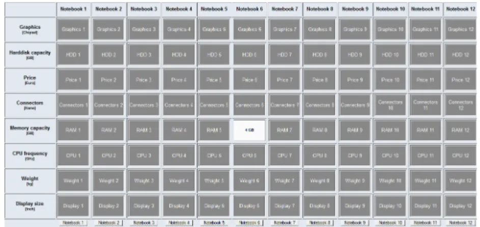
Figure 1: Screenshot of the Mouselab experiment: selection of ‘Expensive Notebook Comput- ers’

Twelve products (columns) are defined by eight attributes (rows) each. All cells are covered unless the mouse cursor is moved over to reveal the underlying attribute value. Only one cell can be opened at a time. Attributes were randomly assigned to rows in every choice problem whereas the location of alternatives was fixed (e.g. Notebook 4 was always displayed in the fourth column).

Notebook 6, see Figure 1). However, once the mouse cursor left an element (e.g.

to move to and uncover another element), the underlying information of the former element was immediately covered again. As in Gabaix et al. (2006), only one element could be viewed at a time. This procedure indicated which element was processed at a time and thus allowed for tracing the information acquisition process.

3.2. Treatment conditions

I used time delays on information acquisition that, in an era of Internet shop- ping, seemed to more appropriately capture the notion of search costs than e.g.

monetary charges. In the no-delay treatment, a cell cover was removed immedi- ately once the mouse cursor entered a matrix element. ⁹ However, in the delay treatments, participants who moved their mouse cursor over an element had to wait for 330, 660 or 1000 milliseconds (ms) until the underlying information was revealed. Although a different range could have been used, two main reasons affected the particular choice of time delays that was implemented. First, the experiment was set-up to isolate the effect of time delays (as a particular imple- mentation of search cost), i.e. varying times delays and holding everything else constant. In that sense there is a natural limit to the range of time delays that could be implemented without changing the perception of the experiment which

9

In order to reduce the noise from accidentally revealed elements (by quickly moving the

mouse cursor across the matrix in the 0ms condition), only opening times ≥ 200ms were

analyzed, which is considered to be the minimum time humans need to perceive the underlying

information (Card et al., 1983; Dumais et al., 2010). It is highly unlikely that this threshold

imposed a serious constraint as 99.3% of the analyzed observations were above 300ms anyway.

would in fact change more than just the time delay. As a treatment without waiting times seems to be a natural lower bound for the range of delay times, the upper bound needed to be selected such that it is not likely to entirely change the qualitative perception of the choice tasks as compared to lower time delays (including the 0ms treatment). Choosing an upper bound of 1000ms (for every single bit of information!) seems to almost, but not yet over-stretch this ceteris paribus condition. ¹⁰

Second, this paper was inspired by the existence of tedious waiting times on natural websites, especially when making product comparisons that involve often switching back and forth between pages. Hence, the experimentally imple- mented range of time delays was supposed to be one that could reasonably be expected to occur in natural online environments. For example, Schurman and Brutlag (2009) who investigated the affect of waiting times for search results for Google and bing used a range of 50ms to 2000ms in their field experiments.

Whereas the time delay treatments were implemented between subjects, the additional treatment dimensions product type (TV-sets or Notebooks) and product costs (price ranges of e 400-700 or e 1000-1300) were varied within sub- jects.

3.3. Hypotheses

Hypothesis 1: The amount of information looked-up decreases in increasing time delays.

It is a well-established empirical result that both monetary search costs and time pressure decrease the amount of information acquired (see section 1). One standard measure to compare search patterns in the decision making literature is Payne’s search index (1976). By distinguishing within-attribute (wATT) from within-alternative (wALT) transitions in information search, the search index is defined as SI = (wALT − wATT)/(wALT + wATT) and thus SI ∈ [−1, 1].

By the specific way of looking-up information every decision can be described by one of four search patterns: attribute-wise (SI < 0), alternative-wise (SI > 0), in a balanced (SI = 0) or in a random pattern. ¹¹ Given a constant number of attributes and alternatives, reducing the number of information elements

10

Although running treatments with substantially longer time delays than 1000ms, e.g.

making participants wait for up to 5000ms (for every single bit of information!), would be interesting in its own right, such very long time delays are likely to qualitatively change the perception of the choice tasks and any results obtained under such extreme conditions would than not be directly comparable to the results obtained under the time delay range imposed.

This would also raise the question of how generalizable such results would be.

11

Whether random search results in a positive or negative search index depends on the

number of attributes M and alternatives N. Actually, SI < 0 ∀M < N and SI > 0 ∀M > N .

Note that the search index is an unbiased measure of the search patterns for this experiment,

as the ratio of the number of attributes and alternatives is constant throughout all treatment

conditions. It is therefore not advantageous to use B¨ ockenholt and Hynan’s (1994) more

complicated strategy measure which is supposed to be used comparing search patterns across

different problem sizes. Furthermore, it is the relative changes of SI between delay treatments

rather than its absolute value that is of interest in this paper.

searched would, conditional on the applied search pattern, result in either lower, equal or higher values of the search index measure. Therefore, it is possible to use observable differences in the search index measure (if any) to infer the search pattern applied by decision-makers. Let l

and l

denote the amount of information searched in situation

and

, respectively. One can draw the following conclusions:

If l

< l

⇒



 

 

SI

< SI

attribute-wise search pattern SI

= SI

balanced or random search pattern SI

> SI

alternative-wise search pattern

Based on previous research findings, it is reasonable to assume that decision- makers are likely to search information elements in an attribute-wise way, start- ing with the most important attribute (e.g. Payne et al., 1993). Henceforth, I will refer to such behavior as following a lexicographic search order. ¹² Due to the chosen form of information presentation in an 12 (alternatives) × 8 (at- tributes) matrix, a lexicographic search order implies that SI increases in the number of elements searched. ¹³ Consequently, as increased search costs reduce the amount of information search, SI is expected to decrease in search costs as well.

Hypothesis 2: Increasing time delays lead to lower values of the search index (i.e. more attribute-wise search patterns).

Regarding the effect of search costs on choice quality Payne et al. (1988) found that time pressure had a clear negative impact on choice quality and sim- ilarly Zakay and Wooler (1984, p279) report a “destructive effect on decision effectiveness”. Although Urbany (1986) did not mention choice quality explic- itly, his results indicate that the joint search costs of monetary charges and delay times had a quality-reducing effect in situations with little prior knowl- edge about the products and narrow price dispersion, i.e. the prices of products were only slightly different from one another. Focusing more on the structure of the choice environment Diehl (2005) showed that, searching for too many alternatives could result in lower choice quality, especially if the environment could be exploited by comparing only very few alternatives. Along the same lines, Gigerenzer and Brighton (2009) also found a significant ‘less is more’ ef- fect, i.e., using heuristic choice rules that deliberately use less information could

12

Importantly, the term ‘lexicographic search order’ should not be mistaken as synonym for lexicographic decision strategies like LEX (Fishburn, 1974) or Take-The-Best (Gigerenzer et al., 1999). Unlike these choice rules that make a specific prediction about choice outcome the term ‘lexicographic search order’ is less restrictive and only describes a specific sequence of information search.

13

If a lexicographic search order is used, reducing the amount of searched information only

means reducing the number of looked-up attributes (but continuing to look-up this reduced set

of attributes from all alternatives). Thus, under the assumption of a lexicographic search order,

revealing less information is expected to result in a shift from alternative-wise to attribute-

wise transitions which due to the very definition of the search index results in lower values of

SI.

substantially improve choice quality. Based on these conflicting findings it is not clear whether reduced information search will necessarily lead to worse levels of choice quality.

The specific two-part set-up applied in this experiment allows for judgments about how well the actual choices fit the decision maker’s preferences. In this article, I will call such a measure of fit choice quality. ¹⁴ Similar to Zakay and Wooler (1984), Johnson and Payne (1985), Coupey and Narayanan (1996), and Chu and Spires (2000), I define choice quality as a relative measure of utility induced by the actually chosen product divided by the potential utility derived from the best available product of a certain choice set. In other words choice quality is a measure of how close a decision maker’s actual choice was to the choice that would have provided the best fit according to his/her preferences over the alternatives in the choice set. For every decision problem separately, choice quality thus is defined as θ = u actual /u max ∈ [0, 1], i.e., how much a decision maker likes the chosen product compared with how much the same decision maker would have liked his/her best option in the choice set, where the best option is evaluated using the decision maker’s preferences. Of course the utility derived from any product crucially depends on the underlying utility function. In this study, I investigate choice quality by using two very prominent utility functions that have often been used in the decision making literature: a compensatory linear weighted-additive and a non-compensatory lexicographic utility model. ¹⁵

Although the two selected utility models are quite different with respect to how information is aggregated, and they could even pick different alterna- tives as the most preferred option of the very same choice set, both models are more accurate in identifying the most preferred option the more information is used before making the decision. Therefore, any decrease in the amount of information looked-up is expected to reduce choice quality. In combination with hypothesis 1 this leads to the prediction that increased search costs are expected to decrease choice quality.

Hypothesis 3: Increasing time delays reduce the quality of choice outcomes.

Note that consistent with Fehr and Rangel (2011) in this paper I treat iden- tifying the search process and estimating the utility models as two separable steps. ¹⁶ First, I am interested in identifying the search process used, while re- maining agnostic about how decision makers aggregate utility. In a second stage, while disregarding the actual choice process, I use two different utility models to

14

What is called choice quality throughout this paper has also been referred to as “choice accuracy” (e.g. Johnson and Payne, 1985) or “decision effectiveness” (Zakay and Wooler, 1984) in the decision-making literature.

15

I am grateful to an anonymous reviewer for the suggestion of adding a lexicographic utility model. Both models and the precise procedures used to estimate them are described in detail in an online appendix.

16

More specifically, Fehr and Rangel (2011, p.8) emphasize that “. . . decision values are

distinct from the experienced utility signal: decision values are forecasts about the experienced

utility signal that will be computed at the time of consumption.”

compute measures for choice quality, i.e. I either assume that decision-makers aggregate utility in a linear or in a lexicographic way. ¹⁷ Whether or not a re- duction in decision quality is substantial depends on the weight (linear utility model) or the attribute rank (lexicographic utility model) of the information elements that are not revealed due to increased search costs. Which elements are disregarded first depends on the search order applied. Remember that a lexicographic search order would start by ignoring the least important bits of information first, thereby resulting only in a marginal decrease in choice quality.

Therefore, finding evidence in line with H3 could be triggered by two con- ditions: either the attributes were almost equally important, i.e. the dispersion in attribute weights was rather small ¹⁸ or decision-makers did not use a lexi- cographic search order (and potentially disregarded more important attributes first). Conversely, the same two conditions would have to be fulfilled simulta- neously in order to reject H3. The decision-makers had to use a lexicographic search order and the dispersion in attribute weights had to be sufficiently large.

Therefore, rejecting H3 (i.e. an increase in search costs does not reduce choice quality) indirectly indicates the use of a lexicographic search order. It should be stressed though that using a lexicographic search order does not automatically mean deriving utility in the way a lexicographic utility model would predict.

Neither does it rule out that decision makers actually could derive their utility in a rather compensatory way in line with a linear utility model.

3.4. Participants and Procedures

All participants had to come to the laboratory twice. In the first session every participant had to make four product choices. The choice problems were presented in a 12 products × 8 attributes matrix display (see Figure 1). In all time delay conditions the participants were asked to choose one product from each of the four choice sets presented to them successively and in random order. Although comparable studies did not use incentive compatible settings, in this experiment one choice round of one participant was randomly selected after finishing all experimental sessions (see Cox et al., 2014). This participant received a voucher that granted a 50% subsidy in case of purchasing exactly the product chosen in his/her ‘winning round’ (e.g. a specific laptop model) and had four weeks to redeem it. Although most laboratory studies on consumer product choice refrain from monetarily incentivizing product choice, the used incentive was supposed to support honest selection behavior along personal preferences.

However, as granting a subsidy could potentially induce a bias towards the selection of more expensive products, only 50% of the actual product price was

17

This approach is often used in the literature on heuristic decision making (e.g. Gigerenzer et al., 1999; Katsikopoulos et al., 2010), where a linear weighted model is used as an important benchmark for decision quality.

18

If the variance in attribute weights is rather small, even using a lexicographic search order

and thereby disregarding only the least important attribute(s) has a strong impact on decision

quality.

provided as a potential payoff. ¹⁹

In the second session the participants engaged in twenty-four binomial prod- uct choices. In order to reduce potential carry-over of product knowledge from the Mouselab search to the binomial choice task a cool-off period of at least twenty-four hours was required between session one and two. As the Mouselab task was considered being more susceptible to potential carry over effects, the task order was not randomized such that the process tracing part was always conducted before the conjoint task (see Funaki et al., 2013). Furthermore, the conjoint task was designed to be robust to any carry over effects (if any). Al- though the attributes necessarily needed to be the same as in the Mouselab task, the optical appearance was entirely different (layout of the screen), all information elements were visible from the start (no need to reveal attribute values) and the attribute values were different from the ones used in the Mouse- lab task. Each of the forty-eight products was specified by carefully varied levels of the same attributes that defined the products used in the Mouselab part. The resulting choice data was used to perform a choice-based conjoint analysis to elicit (i) attribute weights and (ii) attribute ranks that subsequently were used to calculate utility values for each product in the Mouselab choice set. This procedure is based on Lancaster (1966)’s idea of hedonic utility and enabled me to analyze the quality of choice outcomes in the Mouselab stage of the experi- ment. In order to increase the statistical power of the conjoint analysis, but at the same time keep the number of choices per participant manageable without inducing boredom effects, in part two each participant was assigned to make the decisions for either notebooks or TV sets. Consequently, I could calculate the attribute weights for two (out of four) product domains only, which reduced the number of observations for analyzing choice quality and choice efficiency from 315 to 157 (see Table 2).

Eighty-four undergraduate students from the Vienna University of Eco- nomics and Business (Austria) participated in the experiment. The first and the second part of the experiment on average lasted 45 and 25 minutes, respectively.

In addition to participation fees ( e 8 and e 4 for the first and the second part, respectively) participants on average earned e 3.7 from an incentivized ambigu- ity aversion task at the end of part two, resulting in a total average payment of e 15.7 (approx. $20). As the search cost treatment was conducted between subjects, the participants were randomly assigned to the 0ms, 330ms, 660ms or 1000ms delay treatment, resulting in 21, 21, 23 and 19 subjects per condition,

19

Although providing a 50% discount also incentivizes selecting the most expensive model

in a narrow utility maximizing sense, this ‘strategy’ becomes much less salient, as compared

to a 100% discount rate. Actually, participants chose the most expensive products in only

3.2% of all Mouselab choice settings. The ratio of the price of the actually chosen product to

the price of the most expensive product in the choice set did not vary over delay treatments

(Kruskal-Wallis test p = 0.963). This indicates that the used method did not over-incentive

choosing the most expensive product. Simultaneously, it also suggests that the participants

were unlikely to choose randomly as this had resulted in an 8.3% chance of selecting the most

expensive product.

respectively. ²⁰

4. Results

4.1. Testing the hypotheses

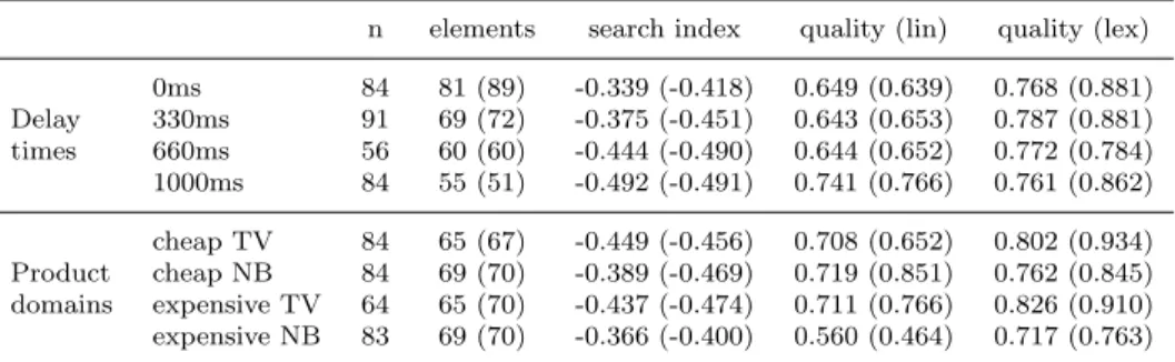
Table 1: Descriptive statistics

n elements search index quality (lin) quality (lex) 0ms 84 81 (89) -0.339 (-0.418) 0.649 (0.639) 0.768 (0.881) Delay 330ms 91 69 (72) -0.375 (-0.451) 0.643 (0.653) 0.787 (0.881) times 660ms 56 60 (60) -0.444 (-0.490) 0.644 (0.652) 0.772 (0.784) 1000ms 84 55 (51) -0.492 (-0.491) 0.741 (0.766) 0.761 (0.862) cheap TV 84 65 (67) -0.449 (-0.456) 0.708 (0.652) 0.802 (0.934) Product cheap NB 84 69 (70) -0.389 (-0.469) 0.719 (0.851) 0.762 (0.845) domains expensive TV 64 65 (70) -0.437 (-0.474) 0.711 (0.766) 0.826 (0.910) expensive NB 83 69 (70) -0.366 (-0.400) 0.560 (0.464) 0.717 (0.763)

Notes: mean values per treatment, medians in parentheses, n: number of observations, elements:

number of unique elements viewed, search index: measure of information processing pattern as defined on page 7, quality (lin): normalized measure of outcome quality based on linear utility model, quality (lex): normalized measure of outcome quality based on lexicographic utility model, 0ms to 1000ms: time to wait until requested information was actually revealed.

Result 1: Time delays significantly reduced the amount of processed informa- tion.

Evidence: In the baseline treatment (no time delay), participants on average opened 81 of 96 totally available elements. Inducing time delays of 330ms, 660ms and 1000ms significantly reduced the amount of processed information to 69, 60 and 55 elements with p = 0.015, p < 0.001 and p < 0.001, respectively (one-sided Wilcoxon Signed-Ranks Test, henceforth osWT). ²¹ These findings were supported by regression analysis (see Table 2).

Result 2: Time delays qualitatively changed the search index in the predicted direction.

Evidence: In the absence of any time delay (0ms treatment) the average search index was −0.339 (median: −0.375) indicating an attribute-wise search

20

This design would have resulted in eighty-four decision processes per product domain.

However, due to a software error, a total of twenty-one observations had to be removed resulting in sixty-four expensive TV set and eighty-three expensive notebook observations.

Testing the distribution across delay treatments with respect to reported gross income and age revealed no significant differences (Kruskal-Wallis test p = 0.921 and p = 0.585, respectively).

21

As the main variables of interest were not normally distributed (Shapiro-Wilk and

Anderson-Darling tests, all p < 0.001), non-parametric tests and Poisson regressions were

used for analyzing the data. In order to deal with the non-independence of four observations

per participant, all non-parametric tests were conducted on subject averages unless stated

otherwise.

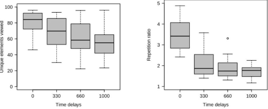
Figure 2: Information acquisition: number of unique elements and repetition ratios by delay treatments

0 330 660 1000

0 20 40 60 80 100

Time delays

Unique elements viewed

0 330 660 1000

1 2 3 4 5

Time delays

Repetition ratio

Both the number of unique elements (of 96 possible, left) and the repetition ratio, i.e. how often one information cell was opened on average (right), were significantly affected by increasing delay times.

pattern. Introducing time delays of 330ms reduced the average search index to

−0.374 (median: −0.406), however the difference was not significant (osWT, p = 0.265). Imposing a time delay of 660ms further reduced the search in- dex to an average of −0.445 (median: −0.505). Although the average again qualitatively shifts in the expected direction, the difference between 330ms and 660ms and between 0ms and 660ms was not significant with p = 0.266 and only marginally significant with p = 0.069 (both osWT), respectively. Further increasing the time delay to 1000ms reduced the search index to an average of

−0.492 (median: −0.478). Whereas the differences between 330ms and 1000ms as well as 660ms and 1000ms were not significant (both osWT with p = 0.152 and p = 0.384, respectively), participants used a significantly more attribute- wise search pattern in the 1000ms treatment than without any delay (osWT, p = 0.038). However, across all treatments, I could not find a statistically sig- nificant result in line with H2 in the regression analysis. Although the delay coefficient qualitatively led in the expected direction, it was not significant. ²² Result 3: Different levels of time delay did not significantly affect the level of choice quality.

Evidence: Recall that choice quality is a generic measure computed as the utility level derived from the actual choice outcome divided by the utility derived from the most preferred outcome (for technical details see online appendix). In order to ensure comparability across product categories (see Figure 4), choice quality was 0-1 normalized for the further analysis. Under perfect information, a decision-maker is expected to choose the best alternative, i.e. the product

22

These regression tables are not reported in the paper but are available from the author.

from which she derives the highest level of utility (resulting in u actual = u max

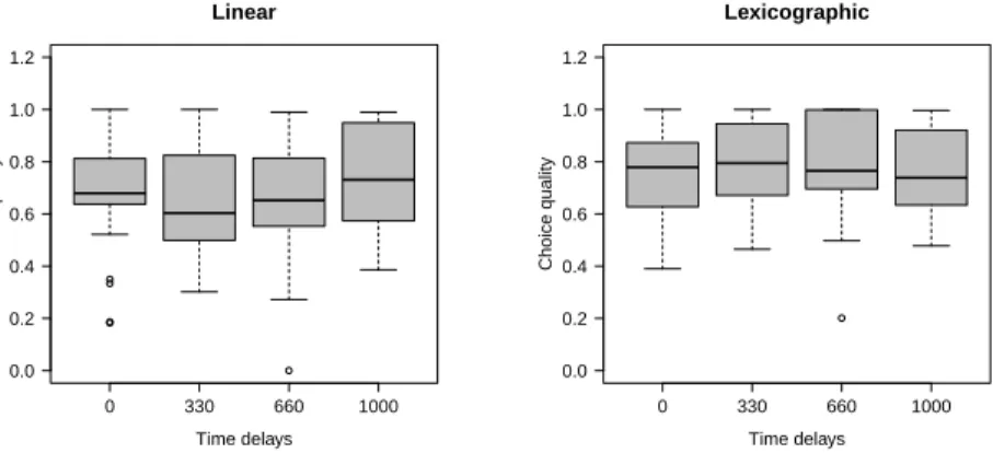
and thus θ = u actual /u max = 1). In the absence of any time delay, participants on average achieved an outcome quality of 0.649 (median: 0.679). The average level of choice quality was reduced to an average of 0.651 (median: 0.603) in the 330ms treatment. This difference is not significant (two-sided Wilcoxon Signed- Ranks Test, henceforth tsWT, p = 0.689). Imposing time delays of 660ms led to an average choice quality of 0.650 (median: 0.652). This level of choice quality is neither significantly different from the level at 0ms nor at 330ms (both tsWT, p = 0.569 and p = 0.631, respectively). Further increasing the time delay to 1000ms resulted in an average choice quality of 0.741 (median: 0.731). Although seemingly larger, the average level of choice quality when imposing 1000ms was not significantly different from the quality levels under 0ms, 330ms or 660ms treatment (all tsWT with p = 0.227, p = 0.173 and p = 0.227, respectively).

Conducting a regression analysis strongly supported the non-parametric results.

Inducing search costs in the form of waiting times for information did not af- fect choice quality at all. This result holds for both implying a linear and a lexicographic utility model (see also Table 2 and Figure 3).

Figure 3: Choice quality

0 330 660 1000

0.0 0.2 0.4 0.6 0.8 1.0 1.2

Linear

Time delays

Choice quality

0 330 660 1000

0.0 0.2 0.4 0.6 0.8 1.0 1.2

Lexicographic

Time delays

Choice quality

Increasing delay times did not affect the levels of relative choice quality at all, irrespective of whether a linear or a lexicographic utility model was implied.

Remember that two conditions had to be satisfied for observing no differences in choice quality across time delays: decision-makers had to use a lexicographic search order and the dispersion in attribute weights had to be sufficiently large.

Using a lexicographic search order means that information elements would be

searched in an attribute-wise manner, starting with the most important at-

tribute. In order to check whether the choice set consisting of real world prod-

ucts was exploitable by a lexicographic search order at all, I followed Fasolo

et al.’s (2007) approach to analyze the resulting hypothetical choice quality if

decision-makers had used only the most important or the four most important

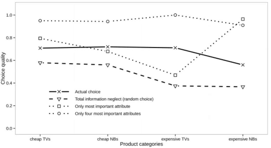
attributes to make a choice. ²³ Only looking-up the most important attribute (see Figure 4: 1 attribute only) resulted in an average hypothetical choice qual- ity of 0.7434 (median: 0.818), which was significantly larger than the average choice quality under random choice (two-sided Wilcoxon Signed-Ranks Test, henceforth tsWT, p < 0.001) and even larger than the overall average empir- ically observed choice quality (tsWT, p = 0.065). Increasing the number of processed attributes (from 1 to 4) on average also improved choice quality (ex- pected to approach unity if all attributes were revealed). ²⁴ Therefore, the choice problems actually used were potentially exploitable by applying a lexicographic search order. Furthermore, Figure 4 also depicts that participants in all prod- uct domains achieved significantly higher levels of choice quality than random choice would have resulted in (tsWT, p < 0.001).

4.2. Supplementary analysis 4.2.1. Search time per element

Analyzing the duration an element was kept open before uncovering the next element revealed substantial differences between the delay time treatments.

Participants on average spent 459ms (median: 435) to process one information element in the no-delay treatment. This processing time increased significantly (tsWT, p < 0.001) to an average of 767ms (median: 703) in the 330ms delay treatment. Further increasing the delay time to 660ms resulted in a significant rise in processing time per element (tsWT, p = 0.006) to on average 879ms (me- dian: 819), which is also significantly larger than under the no-delay condition (tsWT, p < 0.001). Imposing time delays of 1000ms increased the processing time per element to on average 974ms (median: 922), which is significantly larger than under the 0ms or 330ms delay conditions (both tsWT and p < 0.001), but not significantly larger than in the 660ms delay treatment (tsWT, p = 0.153).

Furthermore, the length of the delay time and the time spent per element were strongly correlated (Spearman ρ = 0.694).

4.2.2. Repeated information acquisition

In general, participants made heavy use of the opportunity to re-open any elements at any time. However, the repetition ratio (i.e. how often elements

23

Note that this particular analysis is only informative for utility derived from the linear model. As a lexicographic utility model by definition is non-compensatory, identifying a product only by the first-rated attribute already reveals the best available option. Thus, plotting Figure 4 for hypothetical decisions using a lexicographic utility model would have resulted in choice quality to be at 1 throughout. Observations smaller, yet close to, 1 could only occur in the case of a tie in the first-ranked attribute, in which case the second-ranked attribute would be used to break the tie.

24

Note that it is possible that looking-up fewer attributes results in a higher choice quality

(see Figure 4: In the case of expensive notebooks basing the decision on only the most

important attribute had resulted in a higher choice quality than basing it on the four most

important attributes). This is because adding more information in a non-dominated choice

set could make some alternatives more attractive that would not otherwise be under perfect

information.

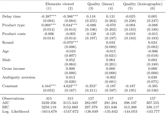
Table 2: Regression results

Elements viewed Quality (linear) Quality (lexicographic)

(1) (2) (3) (4) (5) (6)

Delay time -0.387

-0.386

0.118 0.131 -0.025 0.005

(0.084) (0.084) (0.255) (0.264) (0.238) (0.247) Product type 0.068

0.044

-0.086 -0.070 -0.094 -0.088

(0.014) (0.014) (0.196) (0.202) (0.183) (0.188)

Product costs -0.006 -0.005 -0.128 -0.125 -0.019 -0.015

(0.014) (0.014) (0.197) (0.197) (0.183) (0.183)

Round -0.070

0.033 0.024

(0.006) (0.088) (0.082)

Age -0.010 -0.015 -0.006

(0.007) (0.021) (0.018)

Male 0.052 0.064 0.082

(0.064) (0.201) (0.188)

Gross income 0.000 0.000 0.000

(0.000) (0.000) (0.000)

Ambiguity aversion 0.013 -0.002 0.038

(0.026) (0.081) (0.075)

Constant 4.344

4.623

-0.353

-0.187 -0.187 -0.305

(0.053) (0.167) (0.211) (0.597) (0.195) (0.530)

Observations 315 315 157 157 157 157

AIC 3239.356 3115.343 282.097 291.284 298.107 307.555

BIC 3258.119 3152.869 297.379 321.846 313.388 338.117

Log. Likelihood -1614.678 -1547.672 -136.049 -135.642 -144.053 -143.777

Notes: Poisson regressions with subject-specific random effects; standard errors in parentheses;

significance levels: *** p < 0.01, ** p < 0.05, and * p < 0.1

were re-opened on average) varied drastically between delay treatments (see Figure 2). Whereas one element was processed almost 4 times in the 0ms de- lay treatment (mean: 3.889, median: 3.419), the repetition ratio was virtually halved when a marginal delay of 330ms was imposed (mean: 2.128, median:

1.868, tsWT: p < 0.001). Increasing the delay time to 660ms further decreased the repetition ratio (mean: 1.722, median: 1.668), resulting in a significant difference from the 0ms condition (tsWT, p < 0.001). However, the increase from 330ms to 660ms was not significant (tsWT, p = 0.218). Imposing the maximum delay of 1000ms further reduced the average repetition ratio to 1.697 (median: 1.771). However, this value was not significantly different from the 660ms condition (tsWT, p = 0.361) ²⁵ . Moreover, participants did not treat all information elements equally. The number of look-ups per attribute (includ- ing repetitions) was slightly positively correlated with its respective attribute weight (Spearman, ρ = 0.172) and the four most important attributes were re- vealed significantly more often than the four least important attributes (Sign

25

Whereas the difference between 0ms and 1000ms was highly significant (tsWT, p < 0.001),

the difference between 330ms and 1000ms was only marginally significant (p = 0.053).

Figure 4: Choice quality for hypothetical and observed levels of search intensity by product domain (linear utility model only)

0.0 0.2 0.4 0.6 0.8 1.0

cheap TVs cheap NBs expensive TVs expensive NBs

Product categories

Choice quality

Actual choice

Total information neglect (random choice) Only most important attribute Only four most important attributes

The solid line depicts the average quality of experimentally observed choices which is significantly higher than choosing randomly (dashed line). The dotted lines display the levels of choice quality if only the most important attribute (squares) or the four most important attributes (circles) would have been used to choose a product. This procedure is similar to the one used in Fasolo et al.

(2007).

test, p < 0.05), indicating that more important attributes were revealed more often.

4.2.3. Choice efficiency

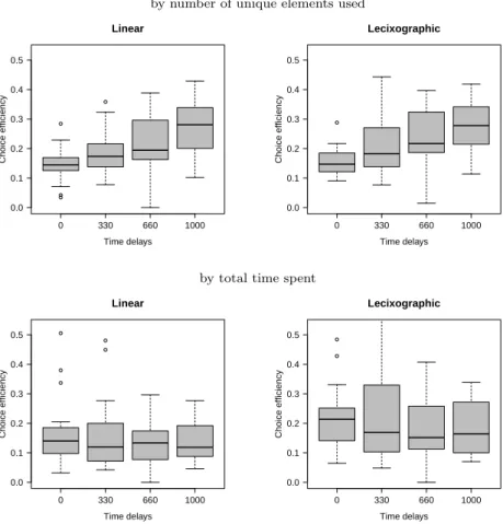
In this paper, two aspects of choice efficiency are reviewed: element-wise and time-wise efficiency. Whereas the former is measured as choice quality divided by the number of unique pieces of information ²⁶ , the latter is measured as choice quality divided by the amount of total time spent on making a choice. ²⁷ As can be inferred from Figure 5 element-wise choice efficiency is positively correlated with the time delays. However, this is not the case when focusing on time-wise choice efficiency. ²⁸

4.2.4. Pattern changes during the search process

Splitting the recorded process data into a first and second half of revealed elements (with repetitions, per choice problem) and analyzing them indepen- dently identified changes in search patterns over time. Not surprisingly, almost

26

This is a conservative measure of choice efficiency as it disregards the dramatic reduction of repeated look-ups under higher time delay treatments. η

=

with e representing the number of unique elements looked-up.

27

η

=

with t being the total time spent on a decision problem before making a choice.

28

Spearman correlations for element-wise efficiency: ρ

= 0.442 and ρ

= 0.341, both

significant with p < 0.01; for time-wise efficiency: ρ

= 0.015 and ρ

= 0.110, both not

significant with p > 0.1.

Figure 5: Choice efficiency by number of unique elements used

0 330 660 1000

0.0 0.1 0.2 0.3 0.4 0.5

Linear

Time delays

Choice efficiency

0 330 660 1000

0.0 0.1 0.2 0.3 0.4 0.5

Lecixographic

Time delays

Choice efficiency

by total time spent

0 330 660 1000

0.0 0.1 0.2 0.3 0.4 0.5

Linear

Time delays

Choice efficiency

0 330 660 1000

0.0 0.1 0.2 0.3 0.4 0.5

Lecixographic

Time delays

Choice efficiency

Increasing time delays had a significant positive effect on choice efficiency, measured as choice quality

per number of unique elements revealed (top row). Choice efficiency defined as choice quality by

the total amount of time spent on the decision problem (including delay times) is not affected by

increasing delay times (bottom row). These results hold for a linear (left) and a lexicographic (right)

utility model.

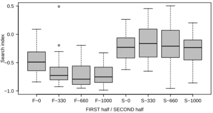
Figure 6: The search index for the first and second half of revealed elements

F−0 F−330 F−660 F−1000 S−0 S−330 S−660 S−1000

−1.0

−0.5 0.0 0.5

FIRST half / SECOND half

Search index

‘F’ denotes the first and ‘S’ the second half of all revealed elements (including repeated look-ups).

In fact, the applied search patterns change significantly during the experimentally observed choice processes.

all unique elements were viewed once during the first half (on average 80%), leaving very few pieces of information entirely unrevealed for the second half.

Only 17% of all unique elements were looked-up for the first time in the second half. Taking a closer look at the search index revealed an interesting change over time. Whereas the average search index for the first half was −0.626, it increased substantially to −0.196 for the second half (see Figure 6). This dif- ference was highly significant (osWT, p < 0.001). Moreover, the variance of the number of elements looked-up per alternative (with repetitions) varied over time. ²⁹ Whereas it was on average 29 for the first half, it increased to 72 in the second half, meaning that search became more selective over time, focusing on a smaller subset of alternatives (osWT, p < 0.001). Consistent with the increasing variance in elements per alternative, I found a decreasing variance regarding the revealed elements per attribute over time (for TV sets and notebooks p = 0.022 and p = 0.049, respectively, both tsWT). Altogether this means that in the second half participants not only focused on fewer alternatives (reduced choice set) but also inspected this subset more closely (on more attributes) than in the first half. Finally, I found no changes in search pattern over time with respect to the time spent per element (all tsWT with p > 0.3).

5. Discussion

5.1. Effects of time delays

Imposing search costs in the form of time delays, in line with previous results, significantly reduced the amount of information acquired, measured by both the

29

Analyzing the variances of look-ups per attribute or alternative is a standard approach in

the strategy selection literature (see Payne et al. (1996); Br¨ oder and Schiffer (2003)).

number of unique elements and all elements including repeated look-ups (Payne et al., 1988, 1996; Kerstholt, 1996; Dhar and Nowlis, 1999; Rieskamp and Hof- frage, 2008). In contrast to the search costs studies of Smith et al. (1982), Zakay and Wooler (1984), Payne et al. (1996), Kerstholt (1996) and Rieskamp and Hoffrage (2008), time delays overall seemed to affect the search index met- ric very little. However, the search index changed substantially throughout the decision process. This was not only highly significant but also very similar to previous findings in magnitude. Splitting the recorded process data into a first and second half of revealed elements (with repetitions, per choice problem) and analyzing them independently identified search pattern changes over time.

Similarly to Verplanken (1993), who found a significant change in the search index from −0.52 to −0.28, the current study identified a shift from −0.61 to

−0.19. Furthermore, consistent with the notion of forming consideration sets (e.g. H¨ aubl and Trifts, 2000; Mehta et al., 2003; Hauser, 2014), participants ini- tially seemed to screen the full choice problem to get a general impression about the available choice options (more attribute-wise search in the first half). After building a consideration set of potentially suitable alternatives they seemed to switch to more intensively analyzing the remaining choice set (more alternative- wise search in the second half). This interpretation is also in line with the observed change of variance of information look-ups per alternative and per attribute. Whereas participants in the first half focused on a broader set of alternatives but fewer attributes, they changed their patterns to investigating fewer alternatives on more attributes in the second half, i.e. analyzing the prod- ucts remaining in the reduced choice set in greater detail (see Payne et al., 1996;

Br¨ oder and Schiffer, 2003).

The strong positive correlation between processing time per element and delay times (Spearman ρ = 0.694) could have three potential causes. Schur- man and Brutlag (2009) found that increasing the artificially imposed delay times caused a direct proportional increase in the users’ response times to click on a search result (“time to click”). Similarly to Schurman and Brutlag’s re- sults, I found that the delay times were strongly externally pacing participants, making them process information elements faster under low and slower under higher time delays. This interpretation is also in line with management litera- ture, which found that employees were significantly reacting to external pacers (Gersick, 1994; Waller et al., 2002), thereby adapting their own speed to the speed of the choice environment. Alternatively, participants could have delib- erately used more time per element to memorize the revealed attribute value better (see Daneman and Carpenter, 1980; Conway et al., 2005). This strat- egy became more and more important when repeatedly looking up information became increasingly more costly under higher delay times. ³⁰ A third plausible

30

It could also be that participants do not only try to memorize information better, but use more demanding procedures to aggregate information (see Johnson and Payne, 1985).

However, it is not likely that increased time delays made decision makers engaged in more

compensatory thinking because in that case — if at all — search patterns became slightly less

compensatory (see result 2).

interpretation would be that participants’ attention drifted away while waiting for an element to be uncovered and it then took them some time to re-focus on the decision problem once the underlying information became available. How- ever, with the data at hand I cannot rule out one alternative or another. Addi- tional research using memory depletion tasks and eye-tracking methods which are beyond the scope of this article could potentially disentangle the above interpretations.

Verplanken (1993) and Verplanken and Weenig (1993) found that time pres- sure reduced the processing time per information element. Payne et al. (1996) found the same effect for incentivized opportunity costs of time. The fact that I find a strong positive correlation between delay times and the processing time per element suggests that there exist important differences between other im- plementations of search costs and delay times. Most likely, this is because of the different incentives to deliberate on the selection of possible search strate- gies. Whereas in a situation with time delays (and also with monetary search costs) there are clear incentives to think twice about the next (costly) informa- tion look-up, in a situation of time pressure the opposite is true. Deliberating about the next move is costly, not the move itself. Consequently, it would only be rational to observe faster information processing for settings of indirectly imposed search costs such as time pressure, whereas just the contrary is true under direct cost conditions as used in the current study. Therefore, my results clearly emphasize that if information search cost is the dimension of interest, implementing them directly (instead of taking an indirect detour of artificially incentivizing the opportunity costs of time monetarily) is of crucial importance.

The current paper only analyzes direct search costs in the form of time delays;

however, the fact that in real life situations it is likely that both direct and indirect search costs occur simultaneously (e.g. experiencing time delays un- der some sort of time pressure), opens up a potentially fruitful area for future research.

5.2. Choice quality and efficiency

In light of the above, it is perhaps not surprising that studies which imposed indirect search costs found that higher time pressure significantly reduced the levels of choice quality (Zakay and Wooler, 1984; Benbasat and Dexter, 1986;

Payne et al., 1988; Hahn et al., 1992). ³¹ However, implementing direct search costs in the form of delay times did not affect choice quality at all. Although higher time delays made participants use fewer information elements, choice quality did not change across delay treatments. This result cannot be explained by random choice, as participants’ choices were of significantly better qual- ity than random choice predictions (both implying the linear and the lexico- graphic model). However, participants appear to have systematically exploited

31

Remember that time pressure in general reduced the time spent to process each informa-

tion element.

the structure of the choice environments. It seems that they successfully sacri- ficed the opportunity of revealing more information, in exchange for the chance of spending more time per revealed piece of information.

Two properties could potentially be used to the decision-makers’ advantage:

a positive correlation of attributes and a sufficiently high dispersion in attribute weights (Bettman et al., 1998; Br¨ oder, 2000; Rieskamp and Otto, 2006; Gigeren- zer and Gaissmaier, 2011). Attributes are deemed to be positively correlated if products that are good (bad) on one attribute also tend to be good (bad) on other attributes. A high positive correlation of attributes could then poten- tially be exploited by comparing all alternatives on just one or few (randomly selected) attributes, as the probability is relatively high that the product per- forming well on a single or a few characteristics also performs well on others. ³² In the context of this study, it is highly unlikely that the attribute correlations of the experimental choice sets were exploited as they were very low. Unlike Fasolo et al. (2007), where the inter-attribute correlations on average were 0.5, the correlation coefficients (Spearman) of the actually used choice environments of the present study were −0.017, −0.067, −0.012 and 0.024 for cheap TV sets, cheap notebooks, expensive TV sets and expensive notebooks, respectively.

As there were almost no attribute correlations to be exploited, the choice environment seems to have provided a sufficiently high dispersion of attribute weights and the participants very likely used an — at least to some extent

— lexicographic search order. Otherwise, they had not been able to achieve relatively high levels of choice quality although using less information (in the higher delay conditions). However, it is worth noting that attribute weights do not have to be extremely skewed. In the current experiment, the weight dispersion was rather moderate for all product domains, yet led to a successful exploitation of this structure. ³³ In real choice environments, retailers or search sites usually describe products by a set of attributes that are expected to play a significant role (e.g. in the case of notebook computers: CPU-speed, RAM- capacity etc.). The extent to which choice efficiency in such an environment could be increased by reducing the amount of information looked-up or the total time spent on making the decision depends on the dispersion of the relative weights of the commonly considered attributes, i.e. how much more important some attributes are perceived compared to others.

Although the main finding of this article is that short time delays (up to 1 second) do not affect choice quality, it is conceivable that implementing much larger time delays, i.e. over 5 or even 10 seconds (per information element!), would have resulted in a drastic drop in choice quality. It is quite likely that such high time delays would significantly reduce the decision makers’ attention (thereby possibly resulting in less accurate choice outcomes) or a substantial

32

The opposite would be true for negative attribute correlations. However, such an envi- ronment cannot be exploited by using the ’right’ decision strategy if it has more than two attributes.

33

The attribute dispersion, as measured by the variance of attribute weights, on average

was 0.120 and 0.211 for TV sets and notebooks, respectively.

degree of choice refusal (see Nielsen, 1993). This, of course, would also be in line with classical search models that trade-off the value gained with the search costs incurred for revealing an additional information element (e.g. Stigler, 1961;

Payne et al., 1993).

5.3. Product space variations

The tested set of metrics did not vary between product domains. Partic- ipants looked-up slightly fewer elements when making choices about TV-sets rather than notebooks, but other than that, the obtained results were stable across product domains. Potentially, participants did not perceive the used product variations as ‘different enough’ to be considered as self-contained prod- uct domains. In fact, both products (and price levels) might have been perceived as belonging to one domain of ‘medium to highly priced consumer electronics’

and thereby reduced any differences between the actually used treatment ma- nipulations. What constitutes the perception of a consumer product choice situation and what makes it being perceived differently from others as well as how such differences could influence the applied search processes seem to out- line an interesting area for future research. Although it seems ex post — given that I do not find substantial differences across product types — that it would have been more advantageous to have used a more stylized environment that provided more experimental control, it is ex ante not trivial to select the right level of abstraction. ³⁴

5.4. Practical implications and avenues for future research

This study has important implications for manufacturers, retailers and mar- keters of consumer durables. Which product is perceived to dominate others, and thus is more likely to be chosen eventually, not only depends on the con- sumer’s preferences but also on the specific process of acquiring and integrating product information. My results indicate that time delays strongly affected how product information was processed and therefore could also have affected which product was chosen as a result of a specific search process. As delay times were manipulated between subjects, it was not possible to identify a direct ‘product switching effect’; however, the significant changes in search behavior most likely affected the final product choice as well (see Branco et al., 2012). More specifi- cally, consumers disregarded more than half of all attributes when experiencing higher delay times. In such a situation, one expects that products are more likely to be chosen if they perform well on a few key characteristics. It then does not

34

I am grateful to an anonymous reviewer to raise this issue. Clearly, how ‘close to reality’

decision making studies should be set up in order not to bias a decision maker’s choice behavior

by overly abstract representations of the choice task needs to be considered on a case by case

basis. Importantly, a more abstract choice environment does not in all circumstances result in

better generalizability. If the decision makers, because of the abstract task, behave differently

than they would in a more natural setting, being more abstract might even backfire as whatever

behaviour is observed, might not be what the researcher was trying to identify, but — at least

in part — a biased artefact of the perceived artificiality of the task.

matter whether or not they perform well on the other (non-key) attributes that are most likely not revealed anyway, under higher time delay conditions. Under shorter time delays however, almost all attributes were processed before making the choice.

Therefore, the profitability of the managerial decision, whether to concen- trate manufacturing and sales resources on products that outperform their direct competitors on only a few attributes, or instead produce models that are more balanced across their attribute values, also depends on the speed of information display of the used online retailing facilities. In that sense, it would be very interesting for future research to analyse the interaction effects of search costs in the form of time delays and time pressure. As technological advances are expected to further reduce delay times of online retailing platforms, products with balanced attribute values could be more successful as compared to those that are only superior regarding a few characteristics. Although delay times did not affect participants’ choices regarding the retailers’ revenue, providing slow online platforms could have severe consequences of a different kind. This study only investigated the effect of waiting times under monopolistic conditions, i.e.

subjects did not have the opportunity to switch to an alternative retailer. As already suggested by Schurman and Brutlag (2009), high delay times could have severe negative implications on the profitability of a search platform provider, when there are alternative providers available. However, investigating the effect of time delays on the competitiveness of online retailers is beyond the scope of this study and remains an interesting opportunity for future research.

What this study also found was that higher time delays made participants keep information elements open for a longer period before revealing the next element. Interestingly, this increase in deliberation time per element was not skewed towards the beginning or the end of a search process, making it unlikely that people developed a search plan upfront before starting to reveal informa- tion. In fact, it seems to be more probable that thinking about the next step (i.e. which information element to reveal next) dominated the observable search behavior.

Although decision-makers reduced the number of information elements used and thereby increased their element-wise choice efficiency, the total time to make a choice (time-wise choice efficiency) was not significantly different throughout all search cost treatments. One way of nudging people towards making choices more efficiently (both by using less information elements and by spending less time) could be to make consumers think about the overall search strategy first.

Spending some time on deliberating what one wants or expects from a product of

a specific domain and subsequently searching accordingly could save the time to

reflect on ‘which element to search next’ for each element separately. It would

therefore be interesting for future research to test ways of nudging decision-

makers to reflect about their wants and a possibly appropriate search strategy

before starting to search. Having clear expectations about the desired product

and a rough plan about how to find it could reduce inefficient over-searching of

the choice environment.