Control Systems II

(1)

Gioele Zardini gzardini@ethz.ch

August 2, 2018

(2)

Abstract

This ”Skript” is made of my notes from the lecture Control Systems II of Dr. Gregor Ochsner (literature of Prof. Dr. Lino Guzzella) and from my lectures as teaching assistant in 2017 for the lecture of Dr. Guillaume Ducard and in 2018 for the lecture of Dr. Jacopo Tani.

This document, should give the chance to repeat one more time the contents of the lecture Control Systems II and practice them through many examples and exercises.

The updated version of the Skript is available on n.ethz.ch/∼gzardini/.

I cannot guarantee on the correctness of what is included in this Skript: it is possible that small errors occur. For this reason I am very grateful to get feedbacks and correc- tions, in order to improve the quality of the literature. An errata version of these notes will always be available on my homepage

Enjoy your Control Systems II!

Cheers!

Gioele Zardini

Version Update:

Version 1: June 2018

(3)

1 Recapitulation from Control Systems I

1.1 Loop Transfer Functions

1.1.1 Standard Feedback Control Loop

The standard feedback control system structure¹ is depicted in Figure 1. This represen-

F(s) C(s)

d(t)

P(s)

n(t)

r(t) e(t) u(t) v(t) η(t) y(t)

−

Figure 1: Standard feedback control system structure.

tation will be the key element for your further control systems studies.

The plant P(s) represents the system you want to control: let’s imagine a Duckiebot.

The variable u(t) represents the real input that is given to the system and d(t) some disturbance that is applyied to it. These two elements toghether, can be resumed into an actuator for the Duckiebot example. The signal v(t) represents thedisturbed input.

The signal η(t) describes the real output of the system. The variable y(t), instead, describes the measured output of the system, which can be eventually measured by a sensor with some noise n(t). In the case of the Duckiebot, this can correspond to the position of the vehicle and its orientation (pose). The feedback controller C(s) makes sure that the tracking errore(t) between the measured output and the referencer(t) approaches zero. F(s) represents the feedforward controller of the system.

Remark. Note the notation: signals in time domain are written with small letters, such as n(t). Transfer functions in frequency domain (Laplace/Fourier transformed) are written with capital letters, such as P(s).

Why transfer functions? In order to make the analysis of such a system easier, the loop transfer functions are defined. In fact, it is worth transforming a problem from the time domain into the frequency domain, solve it, and back transform it into time domain.

The main reason behind this is that convolutions (computationally complex operations which relate signals) are multiplications (through Laplace/Fourier transformation) in the frequency domain.

1Note that multiple versions of this loop exist

(8)

1.1.2 The Gang of Six

The loop gain L(s) is the open-loop transfer function defined by

L(s) =P(s)C(s). (1.1)

The sensitivity S(s) is the closed-loop transfer function defined by S(s) = 1

1 +L(s)

= 1

1 +P(s)C(s).

(1.2)

Remark. Note that the sensitivity gives measure of the influence of disturbancesdon the output y.

The complmentary sensitivity T(s) is the closed-loop transfer function defined by T(s) = L(s)

1 +L(s)

= P(s)C(s) 1 +P(s)C(s).

(1.3)

It can be shown that

S(s) +T(s) = 1. (1.4)

Recalling that a performant controller minimizes the difference between the referenceR(s) and the outputY(s), one can write this difference as an errorE(s). This can be computed as

E(s) =F(s)R(s)−Y(s)

=F(s)R(s)−(η(s) +N(s))

=F(s)R(s)−(P(s)V(s) +N(s))

=F(s)R(s)−(P(s)(D(s) +U(s)) +N(s))

=F(s)R(s)−P(s)D(s)−N(s)−P(s)U(s)

=F(s)R(s)−P(s)D(s)−N(s)−P(s)C(s)E(s).

(1.5)

Furthermore, recalling that we started from E(s), one gets the new equation E(s) =F(s)R(s)−P(s)D(s)−N(s)−P(s)C(s)E(s) (1 +P(s)C(s))E(s) =F(s)R(s)−P(s)D(s)−N(s)

E(s) = F(s)

1 +P(s)C(s)R(s)− P(s)

1 +P(s)C(s)D(s)− 1

1 +P(s)C(s)N(s).

(1.6) This procedure can be applied to each pair of signals of the feedback loop depicted in Figure 1. The following equations can be derived:





 Y(s)

η(s) V(s) U(s) E(s)







= 1

1 +P(s)C(s)







P(s)C(s)F(s) P(s) 1

P(s)C(s)F(s) P(s) −P(s)C(s)

C(s)F(s) 1 −C(s)

C(s)F(s) −P(s)C(s) −C(s)

F(s) −P(s) −1







·



 R(s) D(s) N(s)



. (1.7)

(9)

Exercise 1. A good exercise to practice this procedure could be to derive all the other relations reported in Equation (1.7) on your own.

As you can notice, many terms in the relations introduced in Equation (1.7), are repeated.

Using the defined sensitivity function S(s) (Equation 1.2) and the complementary sensitivity function T(s) (Equation 1.3), one can define four new important transfer functions.

The load sensitivity function is defined as

P(s)S(s) = P(s)

1 +P(s)C(s), (1.8)

and gives us an intuition on how does the disturbance affect the output. The noise sensitivity function is defined as

C(s)S(s) = C(s)

1 +P(s)C(s), (1.9)

and gives us an intuition on how does the noise affect the input. Moreover, one can define two more useful transfer functions:

C(s)F(s)S(s) = C(s)F(s)

1 +P(s)C(s), T(s)F(s) = P(s)C(s)F(s)

1 +P(s)C(s). (1.10) The new introduced four transfer functions together with the sensitivity and the complementary sensitivity functions, describe the so called gang of six.

1.1.3 The Gang of Four

The special case where F(s) = 1 (i.e., no presence feedforward), leads to the equivalence of some of the defined transfer functions. In particular, we are left with four transfer functions:

S(s) = 1

1 +P(s)C(s) sensitivity function, T(s) = P(s)C(s)

1 +P(s)C(s) complementary sensitivity function, P(s)S(s) = P(s)

1 +P(s)C(s) load sensitivity function, C(s)S(s) = C(s)

1 +P(s)C(s) noise sensitivity function.

(1.11)

At this point one may say: I can define these new transfer functions, but why are they necessary? Let’s illustrate this through an easy example.

Example 1. Imagine to deal with a plantP(s) = _s−1¹ and that you control it through a PID controller of the form C(s) =k·^(s−1)_s . You can observe that the plant has a pole at s = 1, which makes it unstable. If one computes the classic transfer functions learned in Control Systems I (Equations (1.1), (1.2), (1.3)), one gets

L(s) = C(s)P(s) = 1

s−1 ·k· (s−1) s = k

s, S(s) = 1

1 +L(s) = s s+k, T(s) = L(s)

1 +L(s) = k s+k.

(1.12)

(10)

You may notice that none of these transfer functions contains the important information about the unstable pole of the plant. However, this information is crucial: if one computes the rest of the gang of four, one gets

P(s)S(s) =

1 s−1

1 + ^k_s = 1

(s−1)(s+k), C(s)S(s) = k· ^(s−1)_s

1 + ^k_s = k(s−1) s+k .

(1.13)

These two transfer functions still contain the problematic term and are extremely useful to determine the influence of the unstable pole on the system, because they explicitly show it.

Exercise 2. Which consequence does the application of a small disturbance d on the system have?

1.1.4 Relations to Performance

By looking at the feedback loop in Figure 1, one can introduce a new variable

ε(t) =r(t)−η(t), (1.14)

which represents the error between the reference signal and the real plant output. One can show, that this error can be written as

ε(s) =S(s)R(s)−P(s)S(s)D(s) +T(s)N(s). (1.15) From this equation one can essentially read:

• For a good reference tracking and disturbance attenuation, one needs a small S(s) (or high L(s)).

• For a good noise rejection, one needs a small T(s) (or small L(s)).

Exercise 3. Derive Equation (1.15) with what you learned in this chapter.

1.1.5 Feed Forward

The feedforward technique complements the feedback one. If on one hand feedback is error based and tries to compensate unexpected or unmodeled phenomena, such as disturbances, noise and model uncertainty, the feedforward technique works well if we have some knowledge of the system (i.e. disturbances, plant, reference). Let’s illustrate the main idea behind this concept through an easy example.

Example 2. The easiest example for this concept, is the one of perfect control. Imagine to have a system as the one depicted in Figure 2.

This is also known as perfect control/plant inversion, where we want to find an inputu(t), such that y(t) = r(t). One can write

Y(s) = P(s)U(s) (1.16)

and hence

R(s) =P(s)U(s)⇒U(s) = P(s)⁻¹R(s). (1.17)

(11)

P(s)

u(t) y(t)

Figure 2: Standard perfect control system structure.

This is not possible when:

• The plant P(s) has right-hand side poles (unstable inverse).

• There are time delays, (non causal inverse): how much of the future output trajectory information we need in order to perform the desired output tracking?

• More poles than zeros, (unrealizable inverse).

• Model uncertainty, (unknown inverse).

But what does it mean for a system to be realizable or causal? Let’s illustrate this with an example.

Example 3. If one has a transfer function with a number of zeros bigger than the number of poles, this represents pure differentiators, which are not causal. Imagine to deal with the transfer function

P(s) = (s+ 2)(s+ 3)

s+ 1 . (1.18)

This transfer function has two zeros and one pole. This can be rewritten as P(s) = (s+ 2)(s+ 3)

s+ 1

= s²+ 5s+ 6 s+ 1

= s(s+ 1) + 4s+ 6 s+ 1

=s+4s+ 6 s+ 1 ,

(1.19)

where s is a pure differentiator. A pure differentiator’s transfer function can be written as the ratio of an output and an input:

G(s) =s= Y(s)

U(s), (1.20)

which describes the time domain equation y(t) = ˙u(t)

= lim

δt→0

u(t+δ_t)−u(t)

δ_t , (1.21)

which confirms us that this transfer function must have knowledge of future values of the input u(t) (from u(t +δt)) in order to react with the current output y(t). This is per definition not physical and hence not realizable, not causal.

(12)

1.2 General Control Objectives

In this section we are going to present the standard control objectives and relate them to what you learned in the course Control Systems I.

But what are the real objectives of a controller? We can subdivide them into four specific needs:

1. Nominal Stability: Is the closed-loop interconnection of a nominal plant and a controller stable?

2. Nominal Performance: Does the closed-loop interconnection of a nominal plant and a controller achieve specific performance objectives?

3. Robust Stability: Is the closed-loop interconnection of any disturbed nominal plant and a controller stable?

4. Robust Performance: Does the closed-loop interconnection of any plant and a controller achieve specific perfomance objectives?

One can essentially subdivide the job of a control engineer into two big tasks:

(I) Analysis: Given a controller, how can we check that the objectives above are satisfied?

(II) Synthesis: Given a plant, how can we design a controller that achieves the objectives above?

Let’s analyse the objectives of a controller with respect to their relation to these two tasks.

1.2.1 Nominal Stability

During the course Control Systems I, you learned about different stability concepts. More- over, you have learned the differences between internal and external stability: let’s recall them here. Consider a generic nonlinear system defined by the dynamics

˙

x(t) = f(x(t)), t ∈R, x(t)∈Rⁿ, f :Rⁿ×R→Rⁿ. (1.22) Definition 1. A state ˆx ∈ Rⁿ is called an equilibrium of system (1.22) if and only if f(ˆx) = 0 ∀t ∈R.

Internal/Lyapunov Stability

Internal stability, also called Lyapunov stability, characterises the stability of the trajec- tories of a dynamic system subject to a perturbation near the to equilibrium. Let now ˆ

x∈Rⁿ be an equilibrium of system (1.22).

Definition 2. An equilibrium ˆx∈Rⁿ is said to be Lyapunov stable if

∀ε >0, ∃δ >0 s.t. kx(0)−xkˆ < δ ⇒ kx(t)−xkˆ < ε. (1.23) In words, an equilibrium is said to beLyapunov stable if for any bounded initial condition and zero input, the state remains bounded.

(13)

Definition 3. An equilibrium ˆx∈ Rⁿ is said to be asymptotically stable in Ω ⊆Rⁿ if it is Lyapunov stable and attractive, i.e. if

t→∞lim(x(t)−x) = 0,ˆ ∀x(0) ∈Ω. (1.24) In words, an equilibrium is said to be asymptotically stable if, for any bounded initial condition and zero input, the state converges to the equilibrium.

Definition 4. An equilibrium ˆx∈Rⁿ is said to be unstable if it is not stable.

Remark. Note that stability is a property of the equilibrium and not of the system in general.

External/BIBO Stability

External stability, also called BIBO stability (Bounded Input-Bounded Output), characterises the stability of a dynamic system which for bounded inputs gives back bounded outputs.

Definition 5. A signal s(t) is said to be bounded, if there exists a finite value B > 0 such that the signal magnitude never exceeds B, that is

|s(t)| ≤B ∀t ∈R. (1.25) Definition 6. A system is said to beBIBO-stable if

ku(t)k ≤ε ∀t ≥0, and x(0) = 0⇒ ky(t)k< δ ∀t≥0, ε, δ ∈R. (1.26) In words, for any bounded input, the output remains bounded.

Stability for LTI Systems

Above, we focused on general nonlinear system. However, in Control Systems I you learned that the output y(t) for a LTI system of the form

˙

x(t) = Ax(t) +Bu(t)

y(t) = Cx(t) +Du(t), (1.27)

can be written as

y(t) = Ce^Atx(0) +C Z t

0

e^A(t−τ)Bu(τ)dτ+Du(t). (1.28)

The transfer function relating input to output is a rational function P(s) =C(sI−A)⁻¹B+D

= bn−1sⁿ⁻¹+bn−2sⁿ⁻²+. . .+b₀

sⁿ+an−1sⁿ⁻¹+. . .+a₀ +d. (1.29) Furthermore, it holds:

• The zeros of the numerator of Equation (1.29) are the zeros of the system, i.e. the values s_i which fulfill

P(s_i) = 0. (1.30)

(14)

• The zeros of the denominator of Equation (1.29) are the poles of the system, i.e.

the values s_i which fulfill det(s_iI−A) = 0, or, in other words, the eigenvalues of A.

One can show, that the following Theorem holds:

Theorem 1. The equilibrium ˆx= 0 of a linear time invariant system is stable if and only if the following two conditions are met:

1. For all λ∈σ(A), Re(λ)≤0.

2. The algebraic and geometric multiplicity of all λ ∈ σ(A) such that Re(λ) = 0 are equal.

Remark. We won’t go into the proof of this theorem, because beyond the scope of the course. As an intuition, however, one can look at Equation (1.28). As you learned in Linear Algebra, the matrix exponential computation can be simplified with help of the diagonalization of a matrix. Moreover, if matrix A is diagonalizable, you can derive a form where you are left with exponential terms of the eigenvalues of A on the diagonal.

If these eigenvalues are bigger than 0, the exponentials, which depends on time, diverge.

If these eigenvalues are smaller than zero, the exponentials converge to 0 (asymptotically stable behaviour). In the case of zero eigenvalues, the exponentials converge, but not to 0 (stable behaviour). If the matrix A is not diagonalizable, i.e. the algebraic and the geometric multiplicity of an eigenvalue do not coincide, one should recall the Jordan form. In this case, some polynomial terms may be multiplied with the exponential ones in the diagonal: this could lead to unstable behaviour (stable vs. unstable because of 0 eigenvalue). For the rigorous proof of the Theorem, go to https://en.wikibooks.org/

wiki/Control_Systems/State-Space_Stability.

1.2.2 Analysis

Which tools do we already know in order to analyze nominal stability? In the course Control Systems I you learned about

• Root locus. In order to recall the root locus method, have a look at Example 4.15, page 123 in [2].

• Bode diagram: the Bode diagram is a frequency explicit representation of the magnitude |L(jω)| and the phase ∠(L(jω)) of a complex number L(jω). Because of graphic reasons, one uses decibel (dB) as unit for the amplitude and degrees as unit for the phase. As a reminder, the conversion reads

XdB = 20·log₁₀(X), X= 10^XdB²⁰ . (1.31) Moreover, stable and unstable poles and zeros have specific consequences on the Bode diagram:

– Poles cause a gradient of −20_decade^dB in the amplitude:

Pole stable unstable Magnitude −20_decade^dB −20_decade^dB

Phase −90^◦ 90^◦

(15)

– Zeros cause a gradient of 20_decade^dB in the amplitude:

Zero stable unstable Magnitude 20_decade^dB 20_decade^dB

Phase 90^◦ −90^◦

An example of a Bode diagram is depicted in Figure 3.

Figure 3: Example of a Bode diagram.

• Nyquist diagram: the Nyquist diagram is a frequency implicit representation of the complex numberL(jω) in the complex plane. An example of a Nyquist diagram is shown in Figure 4.

Remark. In order to draw the Nyquist diagram, some useful limits can be computed:

ω→0limL(jω), lim

ω→∞L(jω), lim

ω→∞∠L(jω). (1.32)

• Nyquist theorem: a closed-loop system T(s) is asymptotically stable if n_c=n₊+n₀

2 (1.33)

holds, where

– n_c: Number of mathematical positive encirclements ofL(s) about critical point

−1 (counterclockwise).

– n₊: Number of unstable poles of L(s) (Re(π)>0).

– n0: Number marginal stable poles of L(s) (Re(π) = 0).

(16)

Figure 4: Example of a Nyquist diagram.

1.2.3 Synthesis: Loop Shaping Plant inversion

As seen in the feedforward example, this method isn’t indicated for non-minimum phase plants and for unstable plants: in those cases this would lead to non-minimum phase or unstable controllers. This method is indicated for simple systems for which it holds

• Plant is asymptotically stable.

• Plant is minimum phase.

The method is then based on a simple step:

L(s) =C(s)·P(s)⇒C(s) = L(s)·P(s)⁻¹. (1.34) The choice of the loop gain is free: it can be chosen such that it meets the desired specifications.

Loop shaping for Non-minimum Phase systems

A non-minimum phase system shows a wrong response: a change in the input results in a change in sign, that is, the system initially lies. Our controller should therefore be patient and for this reason one should use a slow control system. This is obtained by a crossover frequency that is smaller than the non-minimum phase zero. One begins to design the controller with a PI-Controller, which has the form

C(s) = k_p· T_i·s+ 1

T_i·s . (1.35)

(17)

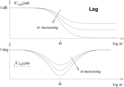
The parameters kp and Ti can be chosen such that the loop gain L(s) meets the known specifications. One can reach better robustness with Lead/Lag elements of the form

C(s) = T ·s+ 1

α·T ·s+ 1. (1.36)

where α, T ∈R⁺. One can understand the Lead and the Lag elements as

• α <1: Lead-Element:

– Phase margin increases.

– Loop gain increases.

• α >1: Lag-Element:

– Phase margin decreases.

– Loop gain decreases.

As one can see in Figure 5 and Figure 6, the maximal benefits are reached at frequencies (ˆω), where the drawbacks are not yet fully developed.

Figure 5: Bodeplot of the Lead Element

The element’s parameters can be calculated as α=

q

tan²( ˆϕ) + 1−tan(ϕ) 2

= 1−sin( ˆϕ)

1 + sin( ˆϕ) (1.37)

and

T = 1 ˆ ω·√

α. (1.38)

(18)

Figure 6: Bodeplot of the Lag Element

where ˆω is the desired center frequency and ˆϕ = ϕ_new−ϕ is the desired maximum phase shift (in rad).

The classic loop-shaping method reads:

1. Design of a PI(D) controller.

2. Add Lead/Lag elements where needed²

3. Set the gain of the controller k_p such that we reach the desired crossover frequency.

Loop shaping for unstable systems

Since the Nyquist theorem should always hold, if it isn’t the case, one has to design the controller such that nc = n++ ⁿ₂⁰ is valid. To remember is: stable poles decrease the phase by 90^◦ and minimum phase zeros increase the phase by 90^◦.

Realizability

Once the controller is designed, one has to look if this is really feasible and possible to implement. That is, if the number of poles is equal or bigger than the number of zeros of the system. If that is not the case, one has to add poles at high frequencies, such that they don’t affect the system near the crossover frequency. One could e.g. add to a PID controller a Roll-Off Term as

C(s) = kp·

1 + 1

T_i·s +Td·s

| {z }

PID Controller

· 1

(τ·s+ 1)²

| {z }

Roll-Off Term

. (1.39)

2L(jω) often suits not the learned requirements

(19)

1.2.4 Performance

Under performance, one can understand two specific tasks:

• Regulation/disturbance rejection: Keep a setpoint despite disturbances, i.e.

keep y(t) at r(t). As an example, you can imagine you try to keep driving your Duckiebot at a constant speed towards a cooling fan.

• Reference Tracking: Reference following, i.e. let y(t) trackr(t). As an example, imagine a luxury Duckiebot which carries Duckiecustomers: a temperature controller tracks the different temperatures which the different Duckiecustomers may want to have in the Duckiebot.

1.2.5 Robustness

All models are wrong, but some of them are useful. (1.40) A control system is said to be robust when it is insensive to model uncertainties. But why should a model have uncertainties? Essentially, for the following reasons:

• Aging: the model that was good a year ago, maybe is not good now. As an example, think of the wheel deterioration which could cause slip in a Duckiebot.

• Poor system identification: there are entire courses dedicated to the art of system modeling. It is not possible not to come to assumptions, which simplify your real system to something that does not perfectly describe that.

1.3 The Bode’s Integral Formula

As we have learned in the previous section, a control systems must satisfy specific performance conditions on the sensitivity functions (also called Gang of Four). As we have seen, the sensitivity function S refers to the disturbance attenuation and relates the tracking errore to the reference signal. As stated in the previous section, one wants the sensitivity to be small over the range of frequencies where small tracking error and good disturbance rejection are desired. Let’s introduce the next concepts with an example:

Example 4. (11.10 Murray) We consider a closed loop system with loop transfer function

L(s) =P(s)C(s) = k

s+ 1, (1.41)

where k is the gain of the controller. Computing the sensitivity function for this loop transfer function results in

S(s) = 1 1 +L(s)

= 1

1 + _s+1^k

= s+ 1 s+ 1 +k.

(1.42)

By looking at the magnitude of the sensitivity function, one gets

|S(jω)|=

r 1 +ω²

1 + 2k+k²+ω². (1.43)

(20)

One notes, that this magnitude |S(jω)|<1 for all finite frequencies and can be made as small as desired by choosing a sufficiently large k.

Theorem 2. Bode’s integral formula. Assume that the loop transfer function L(s) of a feedback system goes to zero faster than ¹_s ass→ ∞, and let S(s) be the sensitivity function. If the loop transfer function has poles p_k in the right-half-plane, then the sensitivity function satisfies the following integral:

Z ∞ 0

log|S(jω)|dω = Z ∞

0

log 1

|1 +L(jω)|dω

=πX p_k.

(1.44)

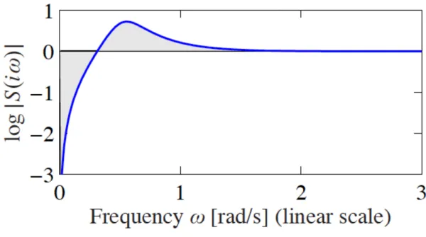
This is usually called the principle of conservation of dirt.

What does this mean?

• Low sensitivity is desirable across a broad range of frequencies. It implies disturbance rejection and good tracking.

• So much dirt we remove at some frequency, that much we need to add at some other frequency. This is also called the waterbed effect.

This can be resumed with Figure 7

Figure 7: Waterbed Effect.

Theorem 3. (Second waterbed formula) Suppose that L(s) has a single real RHP-zeroz or a complex conjugate pair of zeros z =x±jy and hasNp RHP-polespi. Let ¯pi denote the complex conjugate of p_i. Then for closed-loop stability, the sensitivity function must satisfy

Z ∞ 0

ln|S(jω)| ·w(z, ω)dω =π

N p

Y

I=1

|p_i +z

¯

p_i−z|, (1.45)

(21)

where

(w(z, ω) = _z2^2z+ω², if real zero

w(z, ω) = _x2+(y−ω)^x ² +_x2+(y+ω)^x ², if complex zero. (1.46) Summarizing, unstable poles close to RHP-zeros make a plant difficult to control. These weighting functions make the argument of the integral negligible at ω > z. A RHP-zero reduces the frequency range where we can distribute dirt, which implies a higher peak for S(s) and hence disturbance amplification.

1.4 Examples

Example 5. The dynamic equations of a system are given as

˙

x₁(t) = x₁(t)−5x₂(t) +u(t),

˙

x₂(t) = −2x₁(t),

˙

x₃(t) = −x₂(t)−2x₃(t), y(t) = 3x₃(t).

(1.47)

(a) Draw the Signal Diagramof the system.

(b) Find the state space description of the above system.

(22)

Solution.

(a) The Signal Diagram reads

Figure 8: Signal Diagram of the system.

(b) The state space description has the following matrices:

A=





1 −5 0

−2 0 0

0 −1 −2



, b =



 1 0 0



, c= 0 0 3

, d = 0. (1.48)

(23)

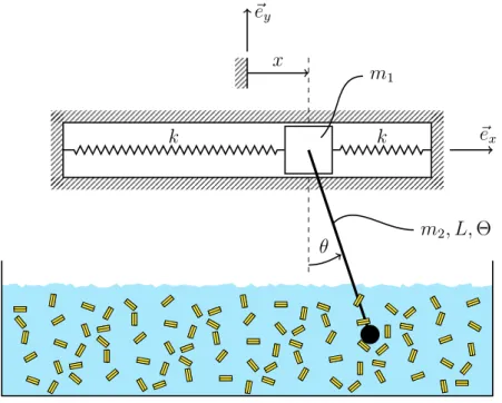
Example 6. Some friends from a new startup of ETH called SpaghETH and want you to help them linearizing the system which describes their ultimate invention. The company is active in the market of the food trucks and sells pasta on the Polyterrasse everyday.

They decided to automate the blending of the pasta in the water by carefully optimizing its operation. A sketch of the revolutionary system is shown in Figure 63.

m₁

m₂, L,Θ x

~e_x

~e_y

k k

θ

Figure 9: Sketch of the system.

The blender is modeled as a bar of mass m₂, length L, and moment of inertia (w.r.t.

center of mass) Θ = ₁₂¹m₂L². The blender is attached to a point mass m₁. In order to deal with possible vibrations that might occur in the system, the mass is attached to two springs with spring constant k.

The equations of motion of the system are given by (m₁+m₂)¨x+ 1

2m₂L

−θ˙²sin(θ)

+ 2kx= 0 m₂

L² 12

θ¨+ 1

2m₂xL˙ θ˙sin(θ) +m₂gL

2 sin(θ) = 0.

(1.49)

a) How would you choose the state space vector in order to linearize this system? Write the system in a new form, with the chosen state space vector.

b) Linearize this system around the equilibrium point where all states are zero except

˙

x(0) =t ∈R is constat in order to find the matrix A.

Hint: Note that no input and no output are considered here, i.e. just the computa- tions for the matrix A are required.

(24)

Solution.

a) The variables x and θ arise from the two equations of motion. Since the equation of motion have order two with respect to these variables, we augment the state and consider also ˙x and ˙θ. Hence, the state space vector s(t) reads

s(t) =





 s₁(t) s₂(t) s3(t) s₄(t)







=





 x(t) θ(t)

˙ x(t) θ(t)˙







. (1.50)

By re-writing the equations of motion with the state space vector one gets

˙ s(t) =







˙ x(t) θ(t)˙

¨ x(t) θ(t)¨







=







s3(t) s₄(t)

1

(m1+m2) · ¹₂m₂Ls₄(t)²sin(s₂(t))−2ks₁(t)

−_L¹ ·(6s₃(t)s₄(t) sin(s₂(t)) + 6gsin(s₂(t)))







:=f (1.51)

b) The linearization of the system reads

A= ∂f

∂s seq.

=







0 0 1 0

0 0 0 1

−_(m^2k

1+m2)

1

2m2Ls4(t)²cos(s2(t))

(m1+m2) 0 ^m²_(m^Ls⁴^sin(s²⁾

1+m2)

0 −^6s³^(t)s⁴^{(t) cos(s}²_L^(t))+6g^cos(s²^(t)) −^6s⁴^{(t) sin(s}_L ²^(t)) −^6s³^{(t) sin(s}_L ²^(t))





 seq

=







0 0 1 0

0 0 0 1

−_(m^2k

1+m2) 0 0 0

0 −^6g_L 0 0





 .

(1.52)

(25)

Example 7. You are given the following matrix:

A =





−3 4 −4 0 5 −8 0 4 −7



. (1.53)

a) Find the eigenvalues of A.

b) Find the eigendecomposition of matrix A, i.e. compute its eigenvectors and determine T and D s.t. A=T DT⁻¹.

c) You are given a system of the form

x(t) = Ax(t) +Bu(t)

y(t) = Cx(t) +Du(t). (1.54) Can you conclude something about the stability of the system?

d) What if you have

A=





−1 0 0

−1 1 0



 (1.55)

instead?

(26)

Solution.

a) The eigenvalues of A should fulfill

det(A−λI) = 0. (1.56)

It follows

det(A−λI) = det





−3−λ 4 −4

0 5−λ −8

0 4 −7−λ





= (−3−λ) det

5−λ −8 4 −7−λ

=−(3 +λ)·[(5−λ)·(−7−λ)−(−24)]

=−(3 +λ)²·(λ−1).

(1.57)

This means that matrix A has eigenvalues

λ_1,2 =−3, λ₃ = 1. (1.58)

b) In order to compute the eigendecomposition of A, we need to compute its eigenvectors with respect to its eigenvalues. The eigenvectors v_i should fulfill

(A−λI)v_i = 0. (1.59)

It holds:

• E_λ₁ =E−3: From (A−λ₁I)·x= 0 one gets the linear system of equations





0 4 −4 0 0 8 −8 0 0 4 −4 0



.

Using the first row as reference and subtracting it from the other two rows, one gets the form





0 4 −4 0

0 0 0 0



.

Since one has two zero rows, one can introduce two free parameters. Letx₁ =s, x₂ =t, s, t∈R. Using the first row, one can recoverx₃ =x₂ =t. This defines the first eigenspace, which reads

E−3 = n



 1 0 0



,



 0 1 1



 o

(1.60) Note that since we have introduced two free parameters, the geometric multiplicity ofλ_1,2 =−3 is 2.

• E_λ₂ =E₁: From (A−λ₂I)·x= 0, one gets the linear system of equations

(27)





−4 4 −4 0 0 4 −8 0 0 4 −8 0



.

Subtracting the second row from the third row results in the form





−4 4 −4 0 0 4 −8 0

0 0 0 0



.

Since one has a zero row, one can introduce a free parameter. Let x₃ = u, u∈R. It follows x₂ = 2t and x₁ =t. The second eigenspace hence reads

E1 = n



 1 2 1



 o

(1.61) Note that since we have introduced one free parameter, the geometric multiplicity ofλ₃ = 1 is 1.

Since the algebraic and geometric multiplicity concide for every eigenvalue ofA, the matrix is diagonalizable. With the computed eigenspaces, one can build the matrix T as

T =





1 0 1 0 1 2 0 1 1



, (1.62)

and D as a diagonal matrix with the eigenvalues on the diagonal:

D=





−3 0 0 0 −3 0

0 0 1



. (1.63)

These T and D are guaranteed to satisfyA =T DT⁻¹.

c) Because ofλ3 = 1>0 one can conclude that the system is unstable in the sense of Lyapunov.

d) Because the new matrix A contains only 0 elements above the diagonal, one can clearly see that its eigenvalues are

λ₁ =−1, λ_2,3 = 0. (1.64)

The eigenvalue λ₁ = −1 leads to asymptotically stable behaviour. The eigenvalue λ_2,3 = 0 has algebraic multiplicity of 2, which means that, in order to have a marginally stable system, its geometric multiplicity should be 2 as well. It holds

• E_λ_2,3 =E₀: From (A−λ_2,3I)·x= 0, one gets the linear system of equations





−1 0 0 0

−1 1 0 0



,

which clearly has x1 = 0, x2 = x2 = 0 and x3 = t ∈ R. Since we introduced only one free parameter, the geometric multiplicity of this eigenvalue is only 1, which means that the system is unstable.

(28)

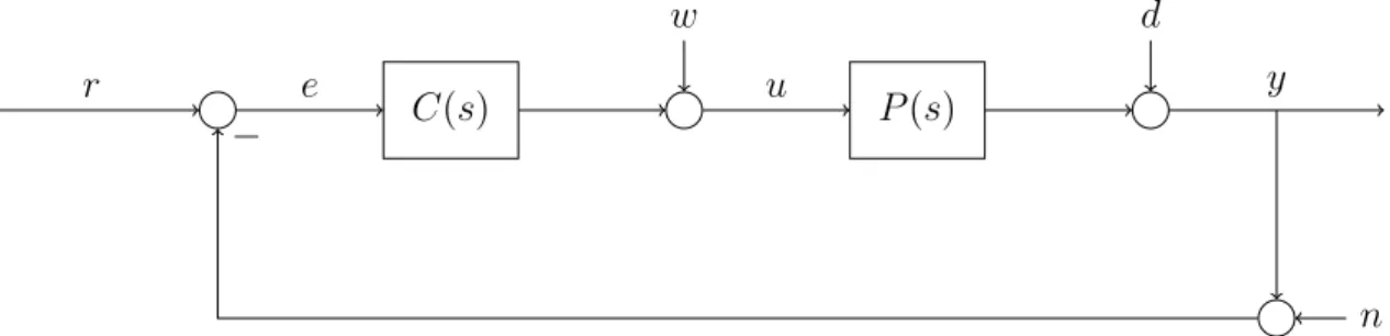
Example 8. Assume that the standard feedback control system structure depicted in Figure 10 is given.

C(s)

w

P(s)

d

r e u y

n

−

Figure 10: Standard feedback control system structure (simplified w.r.t. the lecture notes).

a) Assume that R(s) = 0. What T(s) and S(s) would you prefer? Is this choice possible?

(29)

Solution.

a) If the reference signalR(s) is 0 for all times, the desired output signal Y(s) should be zero for all times as well. Thus, referring to the closed loop dynamics

Y(s) =S(s)·(D(s) +P(s)·W(s)) +T(s)·(R(s)−N(s)), (1.65) the preferred choice would be

T(s) =S(s) = 0. (1.66)

In this case, all the disturbances and noise would be suppressed. However, this choice is not possible. This can be easily checked by looking at the constraint

S(s) +T(s) = 1

1 +L(s) + L(s)

1 +L(s) = 1 +L(s)

1 +L(s) = 1. (1.67) This result has a key importance for the following discussions. In fact, at a fixed frequency s, either S(s) or T(s) can be 0 but not both. In other words, it is not possible to suppress both disturbances and noise in the same frequency band.

(30)

2 Digital Control

2.1 Signals and Systems

A whole course is dedicated to this topic (see Signals and Systems of professor D’Andrea).

A signal is a function of time that represents a physical quantity.

Continuous-timesignals are described by a functionx(t) such that this takes continuous values.

Discrete-timeSignals differ from continuous-time ones because of a sampling procedure.

Computers don’t understand the concept of continuous-time and therefore sample the signals, i.e. measure signal’s informations at specific time instants. Discrete-time systems are described by a function

x[n] =x(n·T_s), (2.1)

where T_s is the sampling time. The sampling frequency is defined asf_s = _T¹

s. One can understand the difference between the two descriptions by looking at Figure 11.

t x(t)

Figure 11: Continuous-Time versus Discrete-Time representation

Advantages of Discrete-Time analysis

• Calculations are easier. Moreover, integrals become sums and differentiations become finite differences.

• One can implement complex algorithms.

Disadvantages of Discrete-Time analysis

• The sampling introduces a delay in the signal (≈e⁻^sTs² ).

• The informations between two samplings, that is betweenx[n] andx[n+ 1], are lost.

Every controller which is implemented on a microprocessor is a discrete-time system.

(31)

2.2 Discrete-Time Control Systems

Nowadays, controls systems are implemented in microcontrollers or in microprocessors in discrete-time and really rarely (see the lecture Elektrotechnik II for an example) in continuous-time. As defined, although the processes are faster and easier, the informations are still sampled and there is a certain loss of data. But how are we flexible about information loss? What is acceptable and what is not? The concept of aliasingwill help us understand that.

2.2.1 Aliasing

If the sampling frequency is chosen too low, i.e. one measures less times pro second, the signal can become poorly determined and the loss of information is too big to reconstruct it uniquely. This situation is called aliasing and one can find many examples of that in the real world. Let’s have a look to an easy example:

Example 9. You are finished with your summer’s exam session and you are flying to Ibiza, to finally enjoy the sun after a summer spent at ETH. You decide to film the turbine of the plane because, although you are on holiday, you have an engineer’s spirit.

You land in Ibiza and, as you get into your hotel room, you want you have a look at your film. The rotation of the turbine’s blades you observe looks different to what it is supposed to be, and since you haven’t drunk yet, there must be some scientific reason. In fact, the sampling frequency of your phone camera is much lower than the turning frequency of the turbine: this results in a loss of information and hence in a wrong perception of what is going on.

Let’s have a more mathematical approach. Let’s assume a signal

x₁(t) = cos(ω·t). (2.2)

After discretization, the sampled signal reads

x1[n] = cos(ω·Ts·n) = cos(Ω·n), Ω =ω·Ts. (2.3) Let’s assume a second signal

x₂(t) = cos

ω+2π T_s

·t

, (2.4)

where the frequency

ω2 =ω+ 2π

T_s. (2.5)

is given. Using the periodicity of the cos function, the discretization of this second signal reads

x₂[n] = cos

ω+2π T_s

·T_s·n

= cos (ω·Ts·n+ 2π·n)

= cos(ω·T_s·n)

=x₁[n].

(2.6)

(32)

Although the two signals have different frequencies, they are equal when discretized. For this reason, one has to define an interval ofgood frequencies, where aliasing doesn’t occur.

In particular it holds

|ω|< π

T_s (2.7)

or

f < 1

2·T_s ⇔f_s >2·f_max. (2.8) The maximal frequency accepted is f = _2·T¹

s and is called Nyquist frequency. In order to ensure good results, one uses in practice a factor of 10.

f < 1

10·T_s ⇔f_s >10·f_max. (2.9) For control systems the crossover frequency should be

f_s ≥10· ω_c

2π. (2.10)

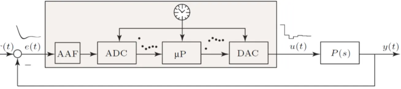
2.2.2 Discrete-time Control Loop Structure

The discrete-time control loop structure is depicted in Figure 12. This is composed of

Figure 12: Control Loop with AAF.

different elements, which we list and describe in the following paragraphs.

Anti Aliasing Filter (AAF)

In order to solve this problem, an Anti Aliasing Filter (AAF) is used. The Anti Aliasing Filter is an analog filter and not a discrete one. In fact, we want to eliminate unwanted frequencies before sampling, because after that is too late (refer to Figure 12).

But how can one define unwanted frequencies? Those frequencies are normally the higher frequencies of a signal ³. Because of that, as AAF one uses normally a low-pass filter.

This type of filter lets low frequencies pass and blocks higher ones⁴. The mathematic formulation of a first-order low-pass filter is given by

lp(s) = k

τ ·s+ 1. (2.11)

wherekis the gain andτ is the time constant of the system. The drawback of such a filter is problematic: the filter introduces additional unwanted phase that can lead to unstable behaviours.

3Keep in mind: high signal frequency means problems by lower sampling frequency!

4This topic is exhaustively discussed in the course Signals and Systems, offered in the fifth semester by Prof. D’Andrea.

(33)

Analog to Digital Converter (ADC)

At each discrete time step t =k·T the ADC converts a voltagee(t) to a digital number following a sampling frequency.

Microcontroller (µP)

This is a discrete-time controller that uses the sampled discrete-signal and gives back a dicrete output.

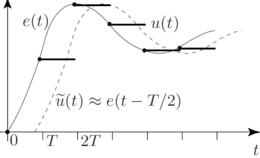
Digital to Analog Converter (DAC)

In order to convert back the signal, the DAC applies a zero-order-hold (ZOH). This introduces an extra delay of ^T₂ (refer to Figure 13).

Figure 13: Zero-Order-Hold.

(34)

2.3 Controller Discretization/Emulation

In order to understand this concept, we have to introduce the concept of z-transform.

2.3.1 The z-Transform

From the Laplace Transform to the z−transform

The Laplace transform is an integral transform which takes a function of a real variable t to a function of a complex variable s. Intuitively, for control systems t represents time and s represents frequency.

Definition 7. The one-sided Laplace transform of a signalx(t) is defined as L(x(t)) =X(s)

= ˜x(s)

= Z ∞

0

x(t)e^−stdt.

(2.12)

Because of its definition, the Laplace transform is used to consider continuous-time signals/systems. In order to deal with discrete-time system, one must derive its discrete analogon.

Example 10. Consider x(t) = cos(ωt). The Laplace transform of such a signal reads L(cos(ωt)) =

Z ∞ 0

e^−stcos(ωt)dt

=−1

se^−stcos(ωt)

∞ 0

− ω s

Z ∞ 0

e^−stsin(ωt)dt

= 1 s − ω

s

−1

se^−stsin(ωt)

∞ 0

+ω s

Z ∞ 0

e^−stcos(ωt)dt

= 1 s − ω²

s²L(cos(ωt)).

(2.13)

From this equation, one has

L(cos(ωt)) = s

s²+ω² (2.14)

Some of the known Laplace transforms are listed in Table 1.

Laplace transforms receive as inputs functions, which are defined in continuous-time. In order to analyze discrete-time system, one must derive its discrete analogue. Discrete time signals x(kT) = x[k] are obtained by sampling a continuous-time function x(t). A sample of a function is its ordinate at a specific time, called the sampling instant, i.e.

x[k] =x(tk), tk =t0+kT, (2.15) where T is the sampling period. A sampled function can be expressed through the mul- tiplication of a continuous funtion and a Dirac comb (see reference), i.e.

x[k] =x(t)·D(t), (2.16)

with D(t) which is a Dirac comb.

(35)

Definition 8. A Dirac comb, also known as sampling function, is a periodic distribution constructed from Dirac delta functions and reads

D(t) =

∞

X

k=−∞

δ(t−kT). (2.17)

Remark. An intuitive explanation of this, is that this function is 1 for t=kT and 0 for all other cases. Since k is a natural number, i.e. k =−∞, . . . ,∞, applying this function to a continuous-time signal consists in considering informations of that signal spaced with the sampling time T.

Imagine to have a continuous-time signal x(t) and to sample it with a sampling periodT. The sampled signal can be described with the help of a Dirac comb as

x_m(t) =x(t)·

∞

X

k=−∞

δ(t−kT)

=

∞

X

k=−∞

x(kT)·δ(t−kT)

=

∞

X

k=−∞

x[k]·δ(t−kT),

(2.18)

where we denote x[k] as the k-th sample ofx(t). Let’s compute the Laplace transform of the sampled signal:

X_m(s) = L(x_m(t))

(a) =

Z ∞ 0

xm(t)e^−stdt

= Z ∞

0

∞

X

k=−∞

x[k]·δ(t−kT)e^−stdt

(b) =

∞

X

k=−∞

x[k]· Z ∞

0

δ(t−kT)e^−stdt

(c) =

∞

X

k=−∞

x[k]e^−ksT,

(2.19)

where we used

(a) This is an application of Definition 7.

(b) The sum and the integral can be switched because the functionf(t) =δ(t−kT)e^−st is non-negative. This is a direct consequence of the Fubini/Tonelli’s theorem. If you are interested in this, have a look at https://en.wikipedia.org/wiki/Fubini%

27s_theorem.

(c) This result is obtained by applying the Dirac integral property, i.e.

Z ∞ 0

δ(t−kT)e^−stdt=e^−ksT. (2.20)

(36)

By introducing the variable z =e^sT, one can rewrite Equation 2.19 as Xm(z) =

∞

X

k=−∞

x[k]z^−k, (2.21)

which is defined as the z−transform of a discrete time system. We have now found the relation between the z transform and the Laplace transform and are able to apply the concept to any discrete-time signal.

Definition 9. The bilateral z-transform of a discrete-time signal x[k] is defined as X(z) =Z((x[k]) =

∞

X

k=−∞

x[k]z^−k. (2.22)

Some of the known z-transforms are listed in Table 1.

x(t) L(x(t))(s) x[k] X(z)

1 ¹_s 1 _1−z¹−1

e^−at _s+a¹ e^−akT _1−e−aT¹ z⁻¹

t _s¹2 kT _(1−z^{T z}⁻¹₋₁

)²

t² _s²3 (kT)² ^T

2z⁻¹(^1+z⁻¹)

(1−z⁻¹)³

sin(ωt) _s2+ω^ω ² sin(ωkT) _1−2z^z−1⁻¹cos(ωT)+z^sin(ωT⁾ ⁻²

cos(ωt) _s2+ω^s ² cos(ωkT) _1−2z^1−z−1⁻¹cos(ωT)+z^cos(ωT⁾⁻²

Table 1: Known Laplace andz−transforms.

Properties

In the following we list some of the most important properties of the z−transform. Let X(z), Y(z) be thez−transforms of the signals x[k], y[k].

1. Linearity

Z(ax[k] +by[k]) = aX(z) +bY(z). (2.23) Proof. It holds

Z(ax[k] +by[k]) =

∞

X

k=−∞

(ax[k] +by[k])z^−k

=

∞

X

k=−∞

ax[k]z^−k+

∞

X

k=−∞

by[k]z^−k

=aX(z) +bY(z).

(2.24)

(37)

2. Time shifting

Z(x[k−k₀]) = z^−k⁰X(z). (2.25) Proof. It holds

Z(x[k−k₀]) =

∞

X

k=−∞

x[k−k₀]z^−k. (2.26) Define m=k−k₀. It holds k =m+k₀ and

∞

X

k=−∞

x[k−k0]z^−k=

∞

X

k=−∞

x[m]z^−mz^−k⁰

=z^−k⁰X(z).

(2.27)

3. Convolution ∗

Z(x[k]∗y[k]) =X(z)Y(z). (2.28)

Proof. Follows directly from the definition of convolution.

4. Reverse time

Z(x[−k]) = X 1

z

. (2.29)

Proof. It holds

Z(x[−k]) =

∞

X

k=−∞

x[−k]z^−k

=

∞

X

r=−∞

x[r]

1 z

−r

=X 1

z

.

(2.30)

5. Scaling in z domain

Z a^kx[k]

=Xz a

. (2.31)

Proof. It holds

Z a^kx[k]

=

∞

X

k=−∞

x[k]z a

^−k

=X z

a

.

(2.32)

(38)

6. Conjugation

Z(x^∗[k]) =X^∗(z^∗). (2.33)

Proof. It holds

X^∗(z) =

∞

X

k=−∞

x[k]z^−k

!∗

=

∞

X

k=−∞

x^∗[k](z^∗)^−k.

(2.34)

Replacing z by z^∗ one gets the desired result.

7. Differentiation in z domain

Z(kx[k]) = −z ∂

∂zX(z). (2.35)

Proof. It holds

∂

∂zX(z) = ∂

∂z

∞

X

k=−∞

x[k]z^−k

linearity of sum/derivative =

∞

X

k=−∞

x[k] ∂

∂zz^−k

=

∞

X

k=−∞

x[k](−k)z^−k−1

=−1 z

∞

X

k=−∞

kx[k]z^−k,

(2.36)

from which the statement follows.

Approximations

In order to use this concept, often the exact solution is too complicated to compute and not needed for an acceptable result. In practice, approximations are used. Instead of considering the derivative as it is defined, one tries to approximate this via differences.

Given y(t) = ˙x(t), the three most used approximation methods are

• Euler forward:

y[k]≈ x[k+ 1]−x[k]

T_s (2.37)

• Euler backward:

y[k]≈ x[k]−x[k−1]

T_s (2.38)

• Tustin method:

y[k]−y[k−1]

2 ≈ x[k]−x[k−1]

T (2.39)

(39)

Exact s = 1

T_s ·ln(z) z =e^s·T^s Euler forward s = z−1

T_s z =s·T_s+ 1 Euler backward s = z−1

z·T_s z = 1 1−s·T_s Tustin s = 2

T_s · z−1

z+ 1 z = 1 +s· ^T₂^s 1−s· ^T₂^s Table 2: Discretization methods and substitution.

The meaning of the variable z can change with respect to the chosen discretization approach. Here, just discretization results are presented. You can try derive the following rules on your own. A list of the most used transformations is reported in Table 2. The different approaches are results of different Taylor’s approximations⁵:

• Euler Forward:

z =e^s·T^s ≈1 +s·Ts. (2.40)

• Euler Backward:

z =e^s·T^s = 1

e^−s·T^s ≈ 1

1−s·T_s. (2.41)

• Tustin:

z= e^s·^Ts²

e^−s·^Ts² ≈ 1 +s·^T₂^s

1−s·^T₂^s. (2.42)

In practice, the most used approach is the Tustin transformation, but there are cases where the other transformations could be useful.

Example 11. You are given the differential relation y(t) = d

dtx(t), x(0) = 0. (2.43)

One can rewrite the relation in the frequency domain using the Laplace transform. Using the property for derivatives

L d

dtf(t)

=sL(f(t))−f(0). (2.44) By Laplace transforming both sides of the relation and using the given initial condition, one gets

Y(s) = sX(s). (2.45)

In order to discretize the relation, we sample with a generic sampling time T the signals.

Forward Euler’s method for the approximation of differentials reads

˙

x(kT)≈ x((k+ 1)T)−x(kT)

T . (2.46)

5As reminder: e^x≈1 +x.

(40)

The discretized relation reads

y(kT) = x((k+ 1)T)−x(kT)

T . (2.47)

In order to compute thez-transform of the relation, one needs to use its time shift property, i.e.

Z(x((k−k₀)T)) =z^−k⁰Z(x(kT)). (2.48) In this case, the shift is of -1 and transforming both sides of the relation results in

Y(z) = zX(z)−X(z)

T = z−1

T X(z). (2.49)

By using the relations of Equation (2.45) and Equation (2.49), one can write s = z−1

T . (2.50)

2.4 State Space Discretization

Starting from the continuous-time state space form

˙

x(t) = Ax(t) +Bu(t)

y(t) = Cx(t) +Du(t), (2.51)

one wants to obtain the discrete-time state space representation x[k+ 1] =A_dx[k] +B_du[k]

y[k] =C_dx[k] +D_du[k]. (2.52) By recalling that x[k + 1] = x((k + 1)T), one can start from the solution derived for continuous-time systems

x(t) = e^Atx(0) +e^At Z t

0

e^−AτBu(τ)dτ. (2.53)

By plugging into this equation t= (k+ 1)T, one gets x((k+ 1)T) =e^A(k+1)Tx(0) +e^A(k+1)T

Z (k+1)T 0

e^−AτBu(τ)dτ (2.54) and hence

x(kT) =e^AkTx(0) +e^AkT Z kT

0

e^−AτBu(τ)dτ. (2.55) Since we want to write x((k+ 1)T) in terms ofx(kT), we multiply all terms of Equation (2.55) by e^AT and rearrange the equation as

eÂ(k+1)Tx(0) =eÂTx(kT)−eÂ(k+1)T Z kT

0

e^−AτBu(τ)dτ. (2.56)