Effects of multi-scale heterogeneity on the simulated evolution of ice-rich permafrost lowlands under a warming climate

(1)

https://doi.org/10.5194/tc-15-1399-2021

Effects of multi-scale heterogeneity on the simulated evolution of ice-rich permafrost lowlands under a warming climate

Jan Nitzbon^1,2,3, Moritz Langer^1,2, Léo C. P. Martin³, Sebastian Westermann³, Thomas Schneider von Deimling^1,2, and Julia Boike^1,2

1Permafrost Research, Alfred Wegener Institute Helmholtz Centre for Polar and Marine Research, Potsdam, Germany

2Geography Department, Humboldt-Universität zu Berlin, Berlin, Germany

3Department of Geosciences, University of Oslo, Oslo, Norway Correspondence:Jan Nitzbon (jan.nitzbon@awi.de)

Received: 12 May 2020 – Discussion started: 2 June 2020

Revised: 20 November 2020 – Accepted: 1 February 2021 – Published: 19 March 2021

Abstract. In continuous permafrost lowlands, thawing of ice-rich deposits and melting of massive ground ice lead to abrupt landscape changes called thermokarst, which have widespread consequences on the thermal, hydrological, and biogeochemical state of the subsurface. However, macro- scale land surface models (LSMs) do not resolve such localized subgrid-scale processes and could hence miss key feedback mechanisms and complexities which affect permafrost degradation and the potential liberation of soil organic carbon in high latitudes. Here, we extend the Cryo- Grid 3 permafrost model with a multi-scale tiling scheme which represents the spatial heterogeneities of surface and subsurface conditions in ice-rich permafrost lowlands. We conducted numerical simulations using stylized model setups to assess how different representations of micro- and meso-scale heterogeneities affect landscape evolution pathways and the amount of permafrost degradation in response to climate warming. At the micro-scale, the terrain was assumed to be either homogeneous or composed of ice-wedge polygons, and at the meso-scale it was assumed to be either homogeneous or resembling a low-gradient slope. We found that by using different model setups and parameter sets, a multitude of landscape evolution pathways could be simulated which correspond well to observed thermokarst landscape dynamics across the Arctic. These pathways include the formation, growth, and gradual drainage of thaw lakes;

the transition from low-centred to high-centred ice-wedge polygons; and the formation of landscape-wide drainage sys- tems due to melting of ice wedges. Moreover, we identified several feedback mechanisms due to lateral transport pro-

cesses which either stabilize or destabilize the thermokarst terrain. The amount of permafrost degradation in response to climate warming was found to depend primarily on the pre- vailing hydrological conditions, which in turn are crucially affected by whether or not micro- and/or meso-scale heterogeneities were considered in the model setup. Our results suggest that the multi-scale tiling scheme allows for simulating ice-rich permafrost landscape dynamics in a more realis- tic way than simplistic one-dimensional models and thus facilitates more robust assessments of permafrost degradation pathways in response to climate warming. Our modelling work improves the understanding of how micro- and meso- scale processes affect the evolution of ice-rich permafrost landscapes, and it informs macro-scale modellers focusing on high-latitude land surface processes about the necessities and possibilities for the inclusion of subgrid-scale processes such as thermokarst within their models.

1 Introduction

Thawing of permafrost in response to climatic change poses a threat to ecosystems, infrastructure, and indigenous com- munities in the Arctic (AMAP, 2017; Vincent et al., 2017;

Schuur and Mack, 2018; Hjort et al., 2018). Pan-Arctic modelling studies have suggested substantial permafrost loss (Lawrence et al., 2012; Slater and Lawrence, 2013) and associated changes in the water and carbon balance of the permafrost region (Burke et al., 2017; Kleinen and Brovkin, 2018; Andresen et al., 2020) within the course of the twenty-

(2)

first century and beyond. The potential liberation of carbon dioxide and methane from thawing permafrost poses a positive feedback to global climate warming (Schuur et al., 2015;

Schneider von Deimling et al., 2015) which is as of yet poorly constrained. Indeed, the macro-scale¹models used to project the response of permafrost to climate warming em- ploy a simplistic representation of permafrost thaw dynamics which only reflects gradual and spatially homogeneous top- down thawing of frozen ground. In particular, such models lack representation of thaw processes in ice-rich permafrost deposits that cause localized and rapid landscape changes called thermokarst (Kokelj and Jorgenson, 2013; Olefeldt et al., 2016). Thermokarst activity is induced on small spatial scales that are below the grid resolution of macro-scale land surface models (LSMs), but it can have widespread effects on the ground thermal and hydrological regimes (Fortier et al., 2007; Liljedahl et al., 2016), on soil erosion (Godin et al., 2014), and on carbon decomposition pathways (Lara et al., 2015; Walter Anthony et al., 2018; Turetsky et al., 2020).

Thermokarst activity can not only induce positive feedback processes leading to accelerated permafrost degradation and landscape collapse (Turetsky et al., 2019; Farquharson et al., 2019; Nitzbon et al., 2020a) but also stabilizing feedbacks, as has been observed in ice-rich terrain (Jorgenson et al., 2015;

Kanevskiy et al., 2017). Overall, thermokarst processes can be considered a key factor of uncertainty in future projections of how the energy, water, and carbon balances of permafrost environments will respond to Arctic climate change (Turet- sky et al., 2019).

Ice-rich permafrost landscapes prone to thermokarst activity are typically characterized by marked spatial heterogeneities that can be linked to the accumulation and melting of excess ice (Kokelj and Jorgenson, 2013). For example, polygonal-patterned tundra in the continuous permafrost zone is underlain by networks of massive ice wedges which give rise to a regular and periodic partitioning of both the surface and the subsurface at the micro-scale (Lachen- bruch, 1962). At the meso-scale, past thermokarst activity has led to a high abundance of thaw lakes in ice-rich permafrost lowlands (Morgenstern et al., 2011). Excess ice melt on the micro-scale can lead to the emergence of thaw features and feedbacks on the meso-scale, such as the formation of drainage networks (Liljedahl et al., 2016), the lateral expansion of thaw lakes (Jones et al., 2011), or the development of thermo-erosional gullies (Godin et al., 2014).

These features have the potential to interact with each other, thereby adding more complexity to the landscape evolution, for example, when a thaw lake drains upon incision of the thermo-erosional gully (Morgenstern et al., 2013). Overall, there is emerging evidence from field observations (Jorgen- son et al., 2006; Farquharson et al., 2019) and remote sensing (Liljedahl et al., 2016; Nitze et al., 2018, 2020) that these

1See Sect. 2.1 and Table 1 for the terminology used in this paper to designate different spatial scales.

subgrid-scale processes crucially affect permafrost degradation pathways and hence also the potential liberation of frozen carbon pools.

Numerical models which represent the “thermokarst- inducing processes” (Nitzbon et al., 2020a) that give rise to the observed complex pathways of permafrost landscape evolution are an important tool to improve our understanding of how subgrid-scale processes affect permafrost degradation in response to climate warming (Rowland et al., 2010; Turetsky et al., 2019). In recent years, substantial progress has been made in the development of numerical models to study the thermal and hydrological dynamics of permafrost terrain on small spatial scales (Painter et al., 2016; Jafarov et al., 2018) and to identify important feedbacks associated with various thermokarst landforms such as ice-wedge polygons (Abolt et al., 2018; Nitzbon et al., 2019; Abolt et al., 2020) or peat plateaus (Martin et al., 2019). The development of numerical schemes simulating ground subsidence resulting from excess ice melt (Lee et al., 2014; Westermann et al., 2016) enabled the assessment of transient changes of thermokarst terrain not only using dedicated permafrost models (Langer et al., 2016;

Nitzbon et al., 2019) but also more broadly using the frame- works of LSMs (Lee et al., 2014; Aas et al., 2019).

Several of these models employed a so-called “tiling approach” to account for subgrid-scale heterogeneities of permafrost terrain. Instead of discretizing extensive landscape domains on a high-resolution mesh, the landscape is parti- tioned into a low number of characteristic landscape units, each of which is associated with a representative “tile” in the model. Thereby, geometrical characteristics of the landscape units (e.g. size and shape, symmetries, and adjacencies) are used to parametrize lateral fluxes among the tiles. For example, Langer et al. (2016) used a two-tile model setup to investigate the effect of lateral heat fluxes in a lake-rich permafrost landscape; Nitzbon et al. (2019) suggested a three-tile setup to represent the micro-scale heterogeneity associated with ice-wedge polygon tundra; and Schneider von Deimling et al.

(2020) applied a five-tile setup to represent the interaction of linear infrastructure such as roads with underlying and surrounding permafrost. So far, the tiling approach has not been applied to simultaneously represent heterogeneities of permafrost landscapes and their interactions across multiple spatial scales.

The overall scope of the present study was to investigate the effect of micro- and meso-scale heterogeneities on the transient evolution of ice-rich permafrost lowlands under a warming climate. Specifically, we addressed the following objectives:

1. to identify degradation pathways and feedback processes associated with lateral fluxes of mass and energy on the micro- and meso-scale,

2. to quantify permafrost degradation in terms of thaw- depth increase and ground subsidence in dependence

(3)

Table 1.Overview of the terminology used in this paper to refer to the spatial scale of permafrost landscape features and processes.

Terminology Superscript Length scale Examples

Subgrid – .10⁵m All mentioned below

Micro µ '10⁰–10¹m Ice-wedge polygons, hummocks Meso m '10²–10³m Thermo-erosion catchments, thaw lakes Macro – '10⁴–10⁵m River delta, LSM grid cell

of the representation of micro- and meso-scale heterogeneities.

For this, we introduced a multi-scale tiling scheme into the CryoGrid 3 permafrost model and conducted numerical simulations for a site in northeastern Siberia under a strong twenty-first century climate-warming scenario (Representa- tive Concentration Pathway 8.5, RCP8.5). We considered different model setups reflecting either the micro-scale heterogeneity associated with ice-wedge polygons, the meso-scale heterogeneity associated with low-gradient slopes, or a combination of both. As a reference case, we considered “single- tile” simulations which emulate the behaviour of macro-scale LSMs. Overall, our goal was to provide a scalable framework for exploring the transient evolution of permafrost landscapes in response to a warming climate which could potentially be incorporated into LSMs to allow for more robust projections of permafrost loss under climate change. The presented simulations should thus be considered as numerical experiments to identify the spatial scales, environmental fac- tors, and feedback mechanisms which affect the degradation of ice-rich permafrost.

2 Methods

2.1 Terminology for spatial scales

Throughout this paper we used a consistent terminology to refer to different characteristic length scales of landscape features and processes. This terminology is summarized in Ta- ble 1.

2.2 Model description

2.2.1 Multi-scale tiling to represent spatial heterogeneity

We used the concept of laterally coupled tiles (Langer et al., 2016; Aas et al., 2019; Nitzbon et al., 2019) to represent subgrid-scale spatial heterogeneities of permafrost terrain.

In general, the tiling concept involves the partitioning of real-world landscapes into a certain number of characteristic units, which are associated with the major surface (or subsurface) heterogeneities found in the landscape. Each of these units is then represented by a single tile in a permafrost model, and multiple tiles can interact through lat-

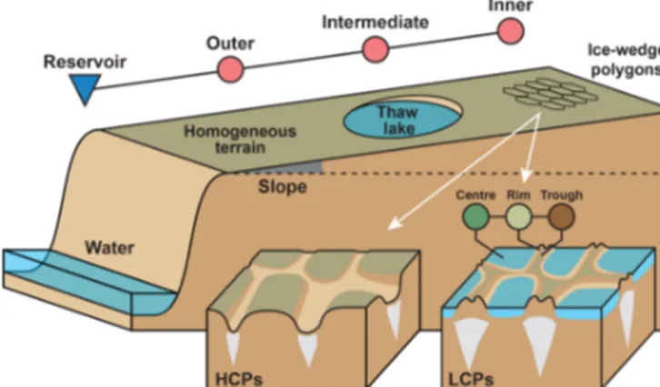
Figure 1.Schematic illustration of ice-rich permafrost lowlands featuring spatial heterogeneity on different scales. At the meso- scale, the terrain is gently sloped and features larger landforms like thaw lakes. At the micro-scale, ice-wedge polygons entail a periodic patterning of the terrain which can have a low-centred (LCPs) or high-centred (HCPs) topography, depending on the grade of degradation. In this study, a tile-based modelling approach is pursued to represent these heterogeneities and investigate their effect on projections of landscape evolution and permafrost degradation.

eral exchange processes. The tiling approach thus allows for simulating subgrid-scale heterogeneities and lateral fluxes in macro-scale models like LSMs without discretizing extensive landscape domains on a high-resolution mesh and hence keeps computational costs at a reasonable level.

For the present study, we applied the tiling concept at multiple scales to represent common spatial heterogeneities of ice-rich continuous permafrost lowlands (see Fig. 1). At the micro-scale, these landscapes are typically characterized by ice-wedge polygons which give rise to a regular patterning of the landscape (see Appendix A for an example site from northeastern Siberia). Here, we adopted the three-tile approach by Nitzbon et al. (2019), which partitions polygonal tundra lowlands into polygon centres, polygon rims, and inter-polygonal troughs. At the meso-scale, tundra lowlands are characterized by gently sloped terrain and often feature abundant thaw lakes that formed in the past due to thermokarst activity (see Appendix A). Here, we used three meso-scale tiles to represent a low-gradient slope which is efficiently drained at its lowest elevation (“drainage point”).

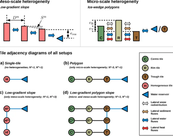
Figure 2 provides an overview of the four model setups which were investigated in this study. These setups differ

(4)

with respect to the number of micro-scale tiles (N^µ) and meso-scale tiles (N^m), the product of which amounts to the total number of tiles (N=N^µ·N^m).

a. Single-tile. This is the simplest case (N^µ=1,N^m=1;

Fig. 2a), which reflects homogeneous surface and subsurface conditions across all spatial scales via only one tile (H). Water can drain laterally into an external reservoir at a fixed elevation (e_res). This setup emulates the one-dimensional representation of permafrost in LSMs and corresponds to the setup used for the simulations conducted by Westermann et al. (2016).

b. Polygon. This setting (N^µ=3, N^m=1; Fig. 2b) reflects the micro-scale heterogeneity associated with ice- wedge polygons via three tiles: polygon centres (C), polygon rims (R), and inter-polygonal troughs (T). The heterogeneity of the surface topography is expressed in different initial elevations of the soil surface of the tiles.

The subsurface stratigraphies of the tiles differ with respect to the depth (dx) and amount (θx) of excess ice, reflecting the subsurface ice-wedge network which is linked to the polygonal pattern at the surface. Lateral fluxes of heat, water, snow, and sediment are enabled among the tiles, and the trough tile is connected to an external water reservoir. This model setup has previously been used by Nitzbon et al. (2019, 2020a).

c. Low-gradient slope. This setup (N^µ=1, N^m=3;

Fig. 2c) reflects a meso-scale gradient of slope S^m, for which the outer (i.e. downstream) tile (H^o) is well- drained into an external reservoir. The intermediate (H^m) and inner (Hⁱ) tiles represent the landscape upstream of the outer tile at constant distances (D^m). The setting assumes a translational symmetry perpendicular to the direction of the slope; i.e. each tile represents the same areal proportion at the meso-scale. Lateral surface and subsurface water fluxes are enabled among the meso-scale tiles, while lateral heat fluxes as treated by Langer et al. (2016) were not considered at this scale.

d. Low-gradient polygon slope. This setup (N^µ=3, N^m=3; Fig. 2d) reflects a meso-scale slope featuring ice-wedge polygons at the micro-scale. Each meso- scale tile includes three micro-scale tiles (C, R, and T), corresponding to the polygon setup described above.

However, only the trough tile of the outer polygon (T^o) is connected to an external reservoir (well-drained), while the intermediate and inner trough tiles are hydro- logically connected along the meso-scale slope.

In the initial configurations, the landscapes were assumed to be undegraded (i.e. the ice-wedge polygons were low- centred, LCPs), and no thaw lakes (water bodies, WBs) were present along the meso-scale slope. However, the model allowed thermokarst features like high-centred polygons

(HCPs) and thaw lakes to develop dynamically as a consequence of excess ice melt at different scales.

2.2.2 Processes representations (CryoGrid 3)

Each of the tiles described in Sect. 2.2.1 was associated with a one-dimensional representation of the subsurface through the CryoGrid 3 permafrost model, which is a phys- ical process-based land surface model tailored for applica- tions in permafrost environments (Westermann et al., 2016).

Heat diffusion with phase change. The numerical model computes the subsurface temperatures (T (z, t )[^◦C]) by solv- ing the heat diffusion equation, thereby taking into account the phase change of soil water (θw[–]) through an effective heat capacity (C_eff(z, T )).

C(z, T )+ρ_wL_sl∂θ_w

∂T

| {z }

Ceff(z,T )

∂T

∂t = ∂

∂z

k(z, T )∂T

∂z

(1)

In Eq. (1)k(z, T )[W K⁻¹m⁻¹] denotes the thermal conductivity andC(z, T )[J K⁻¹m⁻³] denotes the volumetric heat capacity of the soil, both parametrized depending on the soil constituents. ρ_w [kg m⁻³] is the density of water, and L_sl [J kg⁻¹K⁻¹] is the specific latent heat of fusion of water.

The upper boundary condition to Eq. (1) is prescribed as a ground heat flux (Q_g[W m⁻²]), which is obtained by solv- ing the surface energy balance as described in Westermann et al. (2016). The lower boundary condition is given by a constant geothermal heat flux at the lower end of the model domain (Qgeo=0.05 W m⁻²).

Snow scheme. CryoGrid 3 simulates the dynamic build-up and ablation of a snowpack above the surface, heat conduc- tion through the snowpack, changes to the snowpack due to infiltration and refreezing of rain and meltwater, and changes in snow albedo due to ageing. Snow is deposited at an initial density (ρ_snow=250 kg m⁻³), which can increase due to infiltration and refreezing of water.

Hydrology scheme. The model further employs a simple vertical hydrology scheme to represent changes in the ground hydrological regime due to infiltration of rain or meltwater and evapotranspiration (Martin et al., 2019; Nitzbon et al., 2019). Infiltrating water is instantaneously routed downwards through unfrozen soil layers, whose water content is meanwhile set to the field capacity parameter (i.e. the water-holding capacity):θfc=0.5. Once a frozen soil layer is reached, excess water successively saturates the above- lying unfrozen soil layers upwards. Excess water is allowed to pond above the surface, leading to the formation of a surface water body. Surface water is modulated by evaporation as well as lateral fluxes to adjacent tiles or into an external reservoir (see the paragraph on lateral fluxes below). Heat transfer through unfrozen surface water bodies is realized by assuming complete mixing of the water column during the ice-free period (i.e. the water column has a constant temperature profile with depth).

(5)

Figure 2.Overview of the different tile-based model setups used to represent heterogeneity at micro- and meso-scales. An external reservoir (blue triangle) at a fixed elevation (eres) prescribes the hydrological boundary conditions.(a)The single-tile setup used only one tile (homogeneous, H) and does not reflect any subgrid-scale heterogeneity.(b)The polygon setup reflects micro-scale heterogeneity of topography and ground ice distribution associated with ice-wedge polygons via three tiles: a polygon centre (C), polygon rim (R), and inter-polygonal trough (T). The parameterse_Rande_Tindicate the (initial) elevation of rims and troughs relative to the centre. The micro-scale tiles interact through lateral fluxes of heat, water, snow, and sediment.(c)The low-gradient slope reflects meso-scale heterogeneity of an ice-rich lowland via three tiles (H^o,m,i), of which the outer one (H^o) is connected to a draining reservoir. The intermediate (H^m) and inner tiles (Hⁱ) are located at distancesD^malong a low-gradient slopeS^m. The meso-scale tiles interact through lateral surface and subsurface water fluxes.(d)The low-gradient polygon slope incorporates heterogeneities at both micro- and meso-scales via a total of nine tiles.

Excess ice scheme. CryoGrid 3 has an excess ice scheme (“Xice”) which enables it to simulate the ground subsidence as a result of excess ice melt (i.e. thermokarst), following the algorithm proposed by Lee et al. (2014): subsurface grid cells which have an ice content (θ_i) that exceeds the natural porosity (φ_nat) of the soil constituents (θ_m+θo) are treated as excess-ice-bearing cells; once such a cell thaws, the resulting excess water is routed upwards, while above-lying soil constituents are routed downwards and fill the space previously occupied by the excess ice. According to this scheme, thawing of an excess-ice-bearing grid cell of thickness1dresults in a net ground subsidence (1s) which equals

1s=1dθ_i−φ_nat 1−φ_nat

| {z }

θx

, (2)

whereθ_xdenotes the excess ice fraction of the ice-rich soil cell (see Appendix B for a derivation). The excess water is

then treated by the hydrology scheme; i.e. it can either pond at the surface or run off laterally.

Lateral fluxes. The thermal regime and thaw processes in ice-rich permafrost are affected by lateral fluxes of mass and energy at subgrid scales. We used the concept of laterally coupled tiles to represent subgrid-scale heterogeneities of permafrost terrain (see Sect. 2.2.1 for details). We followed Nitzbon et al. (2019) to represent lateral fluxes of heat, water, and snow between adjacent tiles at the micro-scale. Further- more, we included micro-scale advective sediment transport due to slumping, following the approach and using the same parameter values as Nitzbon et al. (2020a). At the meso- scale, we only considered lateral water fluxes, for which we further discriminated between surface and subsurface contri- butions. Both surface and subsurface water fluxes were calculated according to a gradient in water table elevations following Darcy’s law, but the hydraulic conductivities differed considerably (K^subs=10⁻⁵m s⁻¹,K^surf=10⁻²m s⁻¹; see

(6)

Appendix C for details). We did not consider lateral fluxes of heat, snow, and sediment at the meso-scale, as these were assumed to be either negligible on the timescale of interest (heat and sediment) or of uncertain importance (snow). Fi- nally, the model allows for drainage of water into an “external reservoir” at a fixed elevation (e_res) and a constant hydraulic conductivity (K_res=2π K_subs; see supplementary information of Nitzbon et al., 2020a, for details).

2.3 Model settings and simulations 2.3.1 Study area

While the scientific objectives and the modelling concept pursued in this study are general and in principle transfer- able to any ice-rich permafrost terrain, we chose Samoylov Island in the Lena River delta in northeastern Siberia as our focus study area. The island lies in the continuous permafrost zone and is characterized by ice-wedge polygons and surface water bodies of different sizes. The model input data (soil stratigraphies, parameters, meteorological forcing, etc.) were specified based on available observations from this study site.

Details on the study area are provided in Appendix A.

2.3.2 Soil stratigraphies and ground ice distribution The subsurface composition of all tiles was represented via a generic soil stratigraphy (Table 2). The stratigraphy was based on previous studies that applied CryoGrid 3 to the same study area (Nitzbon et al., 2019, 2020a). It consists of two highly porous layers of 0.1 m thickness each which reflect the surface vegetation and an organic-rich peat layer.

Below those, a mineral layer with silty texture follows. An excess ice layer of variable total ice contentθiextends from a variable depth dx down to a depth of 10.0 m. Between the variable excess ice layer and the mineral layer, we assumed an ice-rich intermediate layer of 0.2 m thickness and a total ice content of 0.65. Below the variable excess ice layer follow an ice-poor layer and bedrock down to the end of the model domain. The default ice content assumed for the excess ice layer of homogeneous tiles (no micro-scale heterogeneity) wasθ_i^H=0.75, and the default depth of this layer was d_x=0.9 m. To reflect the heterogeneous excess ice distribution associated with ice-wedge polygons, different ice contents were assumed for the excess ice layers of polygon centres (θ_i^C=0.65), rims (θ_i^R=0.75), and troughs (θ_i^T=0.95). However, the area-weighted mean ice content of ice-wedge polygon terrain is identical to the default value assumed for homogeneous tiles (Table 3).

2.3.3 Topography and geometrical relations among the tiles

Topography. For the single-tile setup (Fig. 2a) the initial elevation of the soil surface was set to 0.0 m. This value does not affect the simulation results, but it serves as a refer-

ence for the variation of the micro- and meso-scale topographies. For the polygon setup (Fig. 2b) we assumed that the rims were elevated by eR=0.2 m relative to the polygon centres, while the troughs had the same initial elevation as the centres (e_T=0.0 m). While this choice of parameters varies slightly from the values assumed in previous studies (Nitzbon et al., 2019, 2020a), it allows for consistent comparability to the setups without micro-scale heterogeneity (see Table 3). The meso-scale topography in the low-gradient slope setup (Fig. 2c) was obtained by multiplying the meso- scale distances (D^m) with the slope of the terrain (S^m). The micro-scale topography of the low-gradient polygon slope setup (Fig. 2d) was obtained by summing up the relative topographic elevations of the meso- and micro-scales.

Geometry. We made simplifying assumptions to determine the adjacency and geometrical relations such as distances and contact lengths among the tiles at the micro- and meso-scale.

These geometrical characteristics determine the magnitude of lateral fluxes between the tiles and only need to be specified if more than one tile is used to represent the respective scale. For the polygon setup with three micro-scale tiles, we assumed a geometry of a circle (centre tile) surrounded by rings (rim and trough tiles), in a manner identical to the setup by Nitzbon et al. (2020a). This geometry is fully defined by specifying the total area (A^µ) of a single-polygonal structure together with the areal fractions (γ_C,R,T) of the three tiles.

Here, we chose values which constitute a compromise between observations from the study area and comparability to the setups without micro-scale heterogeneity (Table 3). For the employed geometry, the micro-scale distances (D^µ) and contact lengths (L^µ) can be calculated according to the for- mulas provided in the supplementary information to Nitzbon et al. (2020a). For the low-gradient slope setups with three meso-scale tiles, we assumed translational symmetry of the landscape in the direction perpendicular to the direction of the gradient. Furthermore, the three meso-scale tiles were assumed to be at equal distances of D^m=100 m from each other. Hence, each meso-scale tile is representative of the same areal fraction of the overall landscape.

2.3.4 Meteorological forcing data

We used the same meteorological forcing dataset which has been used in preceding studies based on CryoGrid 3 for the same study area (Westermann et al., 2016; Langer et al., 2016; Nitzbon et al., 2020a). The dataset spans the period from 1901 until 2100 and is based on downscaled CRUNCEP v5.3 (Climate Research Unit–National Centers for Environmental Prediction) data for the period until 2014.

For the period after 2014, climatic anomalies obtained from CCSM4 (Community Climate System Model) projections for the RCP8.5 scenarios were applied to a 15-year clima- tological base period (2000–2014). A detailed description of how the forcing dataset was generated is provided by West- ermann et al. (2016).

(7)

Table 2.Generic soil stratigraphy used to represent the subsurface composition of all tiles. An ice-rich layer of variable ice content (θ_i) is located at variable depth (dx) from the surface. Note that the effective excess ice content (θx) is linked to the total ice content (θ_i) and the natural porosity (φ_nat) via the relation given in Eq. (2). The soil texture is used to parametrize the freezing-characteristic curve of the respective layer (see Westermann et al., 2016, for details).

Depth from [m] Depth to [m] Mineralθm Organicθo Nat. por.φnat Soil texture Water or iceθ_w⁰ Comment

0 0.1 0 0.15 0.85 Sand 0.85 Vegetation layer

0.1 0.2 0.10 0.15 0.75 Sand 0.75 Organic layer

0.2 dx−0.2 0.25 0.10 0.65 Silt 0.65 Mineral layer

d_x−0.2 d_x 0.20 0.15 0.55 Sand 0.65 Intermediate layer

d_x 10 ^1.05−θ₂ ⁱ ^0.95−θ₂ ⁱ 0.55 Sand θ_i Variable excess ice layer

10 30 0.50 0.05 0.45 Sand 0.45 Ice-poor layer

30 1000 0.90 0 0.10 Sand 0.10 Bedrock

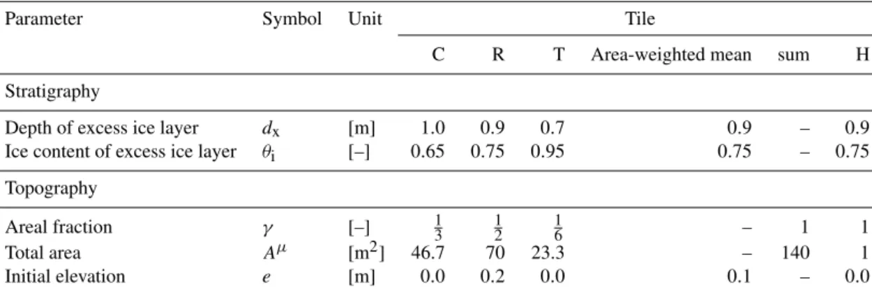
Table 3.Overview of the model parameters for different representations of the micro-scale. Note that on average the polygon tiles (C, R, and T) feature the same excess ice content and depth as the homogeneous tile (H). Setting the area of the homogeneous tile toA^µ=1 m²is an arbitrary choice, as it does not affect the magnitude of the lateral fluxes due to the assumption of translational symmetry.

Parameter Symbol Unit Tile

C R T Area-weighted mean sum H

Stratigraphy

Depth of excess ice layer dx [m] 1.0 0.9 0.7 0.9 – 0.9

Ice content of excess ice layer θ_i [–] 0.65 0.75 0.95 0.75 – 0.75

Topography

Areal fraction γ [–] ¹₃ ¹₂ ¹₆ – 1 1

Total area A^µ [m²] 46.7 70 23.3 – 140 1

Initial elevation e [m] 0.0 0.2 0.0 0.1 – 0.0

2.3.5 Simulations

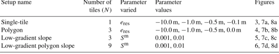
Table 4 provides an overview of all simulations which were conducted for the four different model setups introduced in Sect. 2.2.1. For both the single-tile and the polygon setups we conducted four model runs in which we varied the elevation of the external water reservoir (e_res) in order to reflect a broad range of hydrological conditions. For the low-gradient slope and the low-gradient polygon slope setups we conducted two model runs in which we varied the gradient of the slope (S^m) in order to reflect essentially flat (S^m=0.001) as well as gently sloped terrain (S^m=0.01). In all slope simulations, one tile (H^o and T^o, respectively) was connected to an external reservoir (see Fig. 2c and d;eres= −10.0 m).

The subsurface temperatures of each model run were ini- tialized in October 1999 with a typical temperature profile for that time of year which was based on long-term bore- hole measurements from the study area (Boike et al., 2019).

Using multi-year spin-up periods did not result in significant changes to the near-surface processes investigated in this study so that biases related to the initial subsurface temperature profile can be excluded. The analysed simulation period

was the twenty-first century from January 2000 until Decem- ber 2099.

3 Results

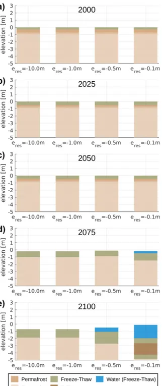
The presentation of the results is structured according to the four different model setups described in Sect. 2.2.1 and vi- sualized in Fig. 2a–d. Figures 3 to 6 provide an overview of the simulated landscape evolution in the four setups by dis- playing the landscape configuration in selected years during the simulation period. While these figures are intended to allow for an intuitive overview of the qualitative behaviour of the model, Figs. 7 and 8 provide a quantitative assessment of permafrost degradation by showing time series of the maximum thaw depths and accumulated ground subsidence for all simulations.

3.1 Single-tile

Figure 3 shows the landscape configuration for selected years throughout the twenty-first century under RCP8.5 for the single-tile setup (see Fig. 2a) under four different hydrological boundary conditions. Until the middle of the simula-

(8)

Table 4.Overview of the parameter variations in the simulations which were conducted for the four different model setups (see Fig. 2). Note that the last value foreresin the single-tile and polygon setups – which reflects poorly drained conditions – was chosen to be 0.1 m less than the mean initial elevation of the respective setting (see Table 3).

Setup name Number of Parameter Parameter Figures

tiles (N) varied values

Single-tile 1 eres −10.0 m,−1.0 m,−0.5 m,−0.1 m 3, 7a, 8a

Polygon 3 eres −10.0 m,−1.0 m,−0.5 m, 0.0 m 4, 7b, 8b

Low-gradient slope 3 S^m 0.001, 0.01 5, 7c, 8c

Low-gradient polygon slope 9 S^m 0.001, 0.01 6, 7d, 8d

tion period (2050) no excess ice melt and associated ground subsidence occur, irrespective of the hydrological conditions (Fig. 3a–c, all columns; Fig. 8a). However, the maximum thaw depths are steadily increasing during that period (see Fig. 7a), with negligible differences between the four runs under different hydrological conditions. Between 2050 and 2075 excess ice melt occurs in all single-tile simulations, leading to ground subsidence of about 0.2 m in the two well- drained cases (Fig. 3d, first and second column), about 0.1 m in the intermediate case (Fig. 3d, third column) and about 0.5 m in the poorly drained case, where excess ice melt leads to the formation of a shallow surface water body (Fig. 3d, fourth column). By 2100 total ground subsidence amounts to about 0.8 m in the well-drained simulations (Fig. 4e, first and second column), and about 1.0 m in the simulation with e_res= −0.5 m, where it is accompanied by the formation of a shallow surface water body (Fig. 4e, third column). In the poorly drained simulation (eres= −0.1 m), excess ice melt proceeds fastest, causing the surface water body to deepen and to reach a depth of about 2 m by 2100; a talik of about 1.5 m thickness has formed underneath the water body by the end of the simulation period (Fig. 3e, fifth column).

Overall, the simulation results indicate that permafrost degradation is strongest as soon as a limitation of water drainage results in the formation of a surface water body. The presence of surface water changes the energy transfer at the surface in different ways. First, it reduces the surface albedo (from 0.20 for barren ground to 0.07 for water), resulting in a higher portion of incoming shortwave radiation. Second, water bodies have a high heat capacity which slows down their freeze-back compared to soil. Third, the thawed saturated deposits beneath the surface water body have a higher thermal conductivity compared to unsaturated deposits, which allows heat to be transported more efficiently from the surface into deeper soil layers.

Interestingly, during the initial phase of excess ice melt which occurs between 2050 and 2075, our simulations suggest a non-monotonous dependence of permafrost degradation on the drainage conditions. This is indicated by the fact that the lowest degradation both in terms of maximum thaw depth and accumulated subsidence is simulated for the intermediate case with e_res= −0.5 m (see Figs. 7a and 8a).

This can likely be attributed to contrasting effects of the hydrological regime in the active layer on thaw depths. When the near-surface ground is unsaturated (as in the simulations witheres= −1.0 m anderes= −10.0 m), the highly porous organic-rich surface layers (see Table 2) have an insulating effect on the ground below due their low thermal conductivity. At the same time, less heat is required to melt the ice contained in the mineral soil layers whose ice content corresponds to the field capacity than would be needed if their pore space was saturated with ice. In the intermediate case withe_res= −0.5 m, the combination of dry, insulating near-surface layers and ice-saturated mineral layers beneath leads to the lowest thaw depths and hence the slowest initial permafrost degradation. However, as soon as a surface water body forms in that simulation (between 2075 and 2100), the positive feedback on thaw described above takes over, resulting in stronger degradation by 2100 compared to the well-drained settings (eres= −1.0 m and eres= −10.0 m), for which no surface water body forms during the simulation period.

In summary, the single-tile simulations illustrate the non- trivial relation between the ground hydrological regime and permafrost thaw and demonstrate the positive feedback associated with surface water body formation resulting from excess ice melt.

3.2 Polygon

Figure 4 illustrates the landscape evolution throughout the twenty-first century under RCP8.5 for the simulations with the polygon setup, i.e. with a representation of micro- scale heterogeneity typical for ice-wedge polygonal tundra. In addition, it shows the geomorphological state of the polygon micro-topography, i.e. whether it is low-centred (LCP), intermediate-centred (ICP), high-centred with inundated troughs (HCPi), high-centred with drained troughs (HCPd), or covered by a surface water body (WB), according to Eqs. (D1) to (D5) in Appendix D. Initially, all simulations feature undegraded ice-wedge polygons with a low-centred micro-topography (Fig. 4a).

Between 2000 and 2025 a shallow surface water body of about 0.5 m depth forms in the poorly drained simulation (e_res=0.0 m) as a result of excess ice melt in the cen-

(9)

Figure 3.Landscape configurations in selected years(a–e)simulated with the single-tile setup (see Fig. 2a) under four different hydrological boundary conditions (left to right).e_resdenotes the elevation of the external water reservoir so that lower values correspond to better drainage.

Figure 4.Landscape configurations in selected years(a–e)simulated with the polygon setup (see Fig. 2b) under four different hydrological boundary conditions (left to right).eresdenotes the elevation of the external water reservoir so that lower values correspond to better drainage. The width of the three tiles corresponds to their areal fractions. Brighter colours reflect higher excess ice contents of the permafrost (see Table 3). Labels indicate the state of the micro- topography according to Eqs. (D1) to (D5)

(10)

Figure 5.Landscape configurations in selected years(a–e)simulated with the low-gradient slope setup (see Fig. 2c) for two different slope gradients (S^m). The outer tile is connected to an external reservoir (eres= −10.0 m) which allows for efficient drainage, while the intermediate and inner tiles can drain only to adjacent tiles.

Figure 6.Landscape configurations in selected years(a–e)simulated with the low-gradient polygon slope setup (see Fig. 2d) for two different slope gradients (S^m). The trough tile of the outer polygon is connected to an external reservoir (e_res= −10.0 m) which allows for efficient drainage. The trough tiles of adjacent polygons are connected to each other and constitute the drainage channels for the entire model domain. Brighter colours reflect higher excess ice contents of the permafrost (see Table 3). Labels indicate the state of the micro-topography according to Eqs. (D1) to (D5).

(11)

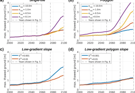
Figure 7.Time series of the maximum thawed-ground thickness throughout the simulation period for all model setups(a–d)and parameter settings.eresdenotes the elevation of the external water reservoir so that lower values correspond to better drainage.S^mdenotes the gradient of the meso-scale slope. To derive the maximum thawed-ground thickness, we first took the maximum annual thaw depth of each tile and then averaged these, weighted according to the areal fractions of the different tiles. We then took the 11-year running mean to obtain a smoothed time series. Dashed grey lines indicate the selected years for which the landscape configuration is explicitly shown in Figs. 3 to 6.

tre, rim, and trough tiles (Fig. 4b, fourth column). The bottom of the water body has a high-centred topography. The landscape configuration does not change much until 2050 (Fig. 4c, fourth column), and the maximum thaw depths and accumulated ground subsidence increase more slowly than in the initial 2 to 3 decades (Figs. 7b and 8b, purple lines). We explain this interim stabilization with the subaqueous transport of sediment from the centres to the rims and from the rims to the troughs, where the additional sediment has an insulating effect on the ice wedge underneath. After 2050 excess ice melt proceeds faster, causing the surface water body to deepen, reaching a depth between about 1 m (centre tile) and more than 2 m (trough tile) by 2075 (Fig. 4 d, fourth column). We explain the acceleration of permafrost degradation at the beginning of the second half of the simulation period (Figs. 7b and 8b, purple lines) by a combination of additional warming from the meteorological forcing and positive feedbacks due to the surface water body (as explained for the single-tile simulation in Sect. 3.1). Until 2100 excess ice melt proceeds further, resulting in a water body depth of 2–4 m and the formation of an extended talik underneath (Fig. 4e, fifth column). By the end of the simulation period, the lake is not entirely bottom-freezing in winter. This constitutes another positive feedback on the degradation rate, since the heat from the ground can be transported much more efficiently through bottom-freezing water bodies than through

those which do not bottom-freeze, due to the higher thermal conductivity of ice compared to that of unfrozen water.

The remaining three simulations show a similar landscape evolution during the first half of the simulation period (2000–

2050), with excess ice melt occurring only in the trough tiles, resulting in a transition from LCP to ICP micro-topography (Fig. 4a–c, first to third column). In contrast to the single- tile setup, the polygon simulations show a monotonous relation between permafrost degradation and drainage conditions during this period. Higher elevations of the external water reservoir (i.e. poorer drainage) result in faster thaw- depth increase (Fig. 7b) and earlier onset of ground subsidence (Fig. 8b). Between 2050 and 2075, substantial excess ice melt occurs in the trough and rim tiles, involving a transition from the ICP to a pronounced HCP micro-topography (Fig. 4d, first to third column). In addition to the positive feedback through surface water formation, the degradation rate in the polygon simulations is accelerated by a positive feedback through lateral snow redistribution. Snow is deposited preferentially in micro-topographic depressions such as initially subsided troughs where it improves the insulation and traps heat in the subsurface during winter, enabling faster and deeper thaw in the subsequent summer. Note that this positive feedback is not represented in the single-tile simulations.

(12)

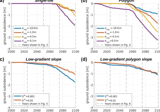
Figure 8.Time series of the accumulated ground subsidence throughout the simulation period for all model setups(a–d)and parameter settings.eresdenotes the elevation of the external water reservoir so that lower values correspond to better drainage.S^mdenotes the gradient of the meso-scale slope. To obtain the accumulated ground subsidence, we first took the difference between the soil surface elevation in each year and the soil surface elevation at the start of the simulation period. We then averaged these differences, weighted according to the areal fractions of the different tiles. Dashed grey lines indicate the selected years for which the landscape configuration is explicitly shown in Figs. 3 to 6.

By 2075 the influence of the drainage conditions on the surface water coverage is most pronounced. While a water body extending over all tiles has formed in the poorly drained simulation (e_res=0.0 m), the polygon centres are (still) elevated above the water table in the intermediate case with e_res= −0.5 m. For e_res= −1.0 m, surface water is found only in the trough tile, while all surface water is drained in the simulation with eres= −10.0 m. Irrespective of the hydrological boundary conditions, permafrost degradation continues in the final decades until 2100. While the high-centred polygon in the well-drained simulation (eres= −10.0 m) re- mains free of surface water (Fig. 4e, first column), surface inundation increases in the runs with intermediate hydrological conditions (Fig. 4e, second and third column), resulting in the formation of a water body of 1–3 m depth underlain by a talik in the simulation with e_res= −0.5 m. However, the water body is (still) bottom-freezing in 2100, in contrast to the water body with floating ice in the simulation with e_res=0.0 m.

Overall, the polygon simulations reveal a marked dependence of the pathways of landscape evolution and associated permafrost degradation on the hydrological conditions, consistent with previous results under recent climatic conditions (Nitzbon et al., 2019).

3.3 Low-gradient slope

While the single-tile and polygon simulations illustrated general feedbacks due to excess ice melt and micro-scale lateral fluxes, they cannot reflect heterogeneous landscape dynamics at the meso-scale. The simulations with the low-gradient slope setup illustrate how meso-scale lateral water fluxes in gently sloped terrain give rise to diverse pathways of landscape evolution and how these depend on the slope gradient (S^m).

Figure 5 shows the landscape evolution throughout the twenty-first century for the simulations with the low-gradient slope setup, i.e. with a meso-scale representation according to a slope but without micro-scale heterogeneities. Irrespec- tive of the slope gradient, the simulated evolution of the outer tiles is very similar to that of the well-drained single-tile simulations (e_res= −10.0 m anderes= −1.0 m) throughout the entire simulation period (compare Fig. 3, first and second columns, with Fig. 5, first and fourth column). The outer tiles are stable through the first half of the simulation period. Dur- ing the second half, excess ice melt sets in, and the ground subsides at an increasing rate, reaching an accumulated subsidence of about 0.8 m by 2100. The similarity to the well- drained single-tile simulations can be explained by the fact that the outer tile is very efficiently drained (e_res= −10.0 m)

(13)

such that the lateral water input from the intermediate tile is directly routed further into the external reservoir. Hence, the

“upstream” influence on the outer tile becomes negligible.

For both slope gradients, the evolution of the intermediate tile is similar to that of the inner tile. However, the evolution of the two tiles is different among the two simulations for different slope gradients. For the lower slope gradient (S^m=0.001), which reflects an essentially flat landscape, melting of excess ice and associated ground subsidence occur during the first half of the simulation period, and a shallow layer of surface water (about 0.2 m) forms in these tiles (Fig. 5a–c, second and third column). By 2050, the soil surface in the intermediate and inner tiles has subsided below the surface elevation of the outer tile such that the initial slope is dissipated. After 2050 excess ice melt proceeds faster, and the surface water body in the intermediate and inner tiles reaches a depth of almost 1 m by 2075 (Fig. 5 d, second and third column). The permafrost table in these tiles is lowered by about 2 m relative to its initial posi- tion. Between 2075 and 2100 a talik forms beneath the water body in the two inland tiles (Fig. 5 e, second and third column), which by 2100 reaches a depth of about 2.0 m. The ground subsidence in the outer tile during the second half of the simulation enables surface and subsurface water transport from the intermediate tile into the external reservoir and thus leads to a lowering of the water level of the water body in the intermediate and inner tiles (Fig. 5d–e). By 2100 the water body depth is about 1.2–1.5 m, which is significantly lower than the water body of about 2.0 m depth which forms in the poorly drained single-tile simulations (Fig. 3 e, fourth column). This difference in water body depths is despite the fact that excess ice melt and surface water formation set on several decades earlier in the low-gradient slope simulation than in the poorly drained single-tile simulation. These different pathways of water body and talik formation illustrate that there is no linear relationship between the water body depth and talik extent, since lateral interactions at the meso- scale can give rise to different transient dynamics.

For the higher slope gradient (S^m=0.01), which reflects moderately sloped terrain, initial excess ice melt occurs in the intermediate and inner tiles between 2000 and 2025, and by 2050 these have subsided by about 0.2 m (Fig. 5, fifth and sixth column), similar to the simulation withS^m=0.001. By 2075, ground subsidence has reached about 0.5 m in the intermediate and inner tiles. The overall shape of the slope does not change much because excess ice melt occurs also in the outer tile during that time. By 2100, the intermediate and inner tile have subsided by about 1.2 m, and the outer tile has subsided by about 0.8 m, resulting in a slightly concave slope. The presence of a thin layer of surface water in the intermediate and inner tiles in the years 2025, 2075, and 2100 indicates a wetter hydrological regime compared to the outer tile. However, as the moderate slope is sustained throughout the simulation, it facilitates drainage of surface water and precludes the formation of a surface water body as is the case

in the simulation with the flatter topography (S^m=0.001).

We suspect, however, that if the simulations would be pro- longed beyond 2100, the excess ice melt in the intermediate and inner tiles would likely continue at a faster rate than in the outer tile and that this would result in the reversal of the initial slope and promote the formation of an inland surface water body.

While the overall dynamics of the three-tile slope simulations could also be reflected using a two-tile setup, we would like to point to the small but significant differences between the evolution of the intermediate tile and the inner tile. For both slope gradients, the intermediate tile shows a slightly stronger degradation rate than the inner tile. This can be explained due to the additional water input from the inner tile which sustains saturated conditions in the near-surface soil layers during the thawing season. The inner tile in turn lacks this lateral water input and is thus more likely to develop dry, thermally insulating conditions in the near-surface soil.

Overall, the slope gradient (S^m) has a similar influence on permafrost degradation in the low-gradient slope setup, as the elevation of the external reservoir (e_res) has in the single- tile simulations (see Figs. 7a and c and 8a and c). This can be attributed to the direct influence of the slope gradient on drainage efficiency. Due to the positive feedbacks related to the formation of a surface water body, the overall permafrost degradation in the setting withS^m=0.001 is almost twice as much as in the setting withS^m=0.01 for which no water body forms. We note that the maximum thawed ground and the accumulated ground subsidence by 2100 in both low- gradient slope simulations are within those simulated for the two extreme settings in the single-tile simulations.

3.4 Low-gradient polygon slope

Finally, we consider the most complex setup, which reflects gently sloped polygonal tundra via nine tiles, incorporating heterogeneities on both the micro- and the meso-scale. Fig- ure 6 shows different stages of the simulated landscape evolution in the low-gradient polygon slope setup throughout the twenty-first century for two different slope gradientsS^m.

Like the outer tiles in the low-gradient slope setup, the outer polygons show an evolution which is very similar to that of the well-drained (single-) polygon simulation with eres= −10.0 m, irrespective of the slope gradient (compare Fig. 6, first and fourth column, with Fig. 4, first column):

until 2050 initial excess ice melt occurs in the trough tiles, entailing a transition from LCP to ICP topography; during the second half of the simulation period, permafrost degradation proceeds at an increasing rate and brings about a transition to a pronounced HCP topography with the troughs hav- ing subsided by about 2 m. Again, the similarity between the outer-polygon evolution and the well-drained single-polygon evolution can be explained by the efficient drainage of the outer-polygon troughs which leads to a negligible upstream influence.

(14)

For the lower slope gradient (S^m=0.001), the intermediate and inner polygons show an evolution which is similar to each other but different from each of the single-polygon simulations (compare Fig. 4 with Fig. 6, second and third column). Between 2000 and 2025 excess ice melt in the rim and trough tiles leads to ponding of surface water in the intermediate and inner polygons (Fig. 6b, second and third column) with the soil surface of the polygon centre being close to or elevated above the water table. Besides a lowering of the water table, the configuration of these polygons does not change much until 2050 (Fig. 6c, second and third column) when both have developed an HCPi topography, i.e. inundated rims and troughs which subsided below the level of the centres. Between 2050 and 2075, excess ice melt continues, leading to a pronounced high-centred topography (Fig. 6d, second and third column). Meanwhile, the surface water dis- appears from the rim and trough tiles, as a consequence of marked excess ice melt in the outer-polygon rim and troughs tiles during that period (Fig. 6d, first column). The soil surface elevation of the trough tiles increases from the outer towards the inner polygon, allowing for efficient drainage of the entire landscape. Between 2075 and 2100 all three polygons show a similar evolution, resulting in pronounced high- centred topographies with troughs about 2 m deep and rims that subsided by about 1 m in total. Note that between 2075 and 2100 the troughs of the intermediate and inner polygons subsided more than that of the outer polygon, resulting in an decreased drainage efficiency. Hence, surface water starts to pond again in the intermediate and inner troughs (Fig. 6e, second and third column). Overall, the low-gradient polygon slope simulation with S^m=0.001 shows a transient phase in which the formation of a water body is initiated, but its growth is impeded due to the formation of efficient drainage pathways through the subsiding troughs in the outer (“downstream”) polygon.

The simulated landscape evolution for the moderate slope gradient (S^m=0.01) differs from that for the lower slope gradient during the first half of the simulation period. Until 2025, excess ice melt is restricted to the trough tiles, leading to a transition from LCP to ICP topography in all three polygons (Fig. 6b, fifth and sixth column). In the intermediate and inner polygons, permafrost degradation proceeds faster than in the outer polygon such that these develop a HCPd topography by 2050. The faster degradation can be explained by the overall wetter hydrological regime compared to the very efficiently drained outer polygon. However, the meso- scale slope still allows for sufficient drainage of surface water such that – in contrast to the simulation withS^m=0.001 – the ponding of surface water is mostly precluded (Fig. 6c, fifth and sixth column). During the second half of the simulation period, the evolution of the polygons is very similar for both slope gradients. Ice-wedge degradation proceeds at an increasing pace between 2050 and 2100, resulting in polygons with pronounced HCP topography. While the troughs of the outer polygons are efficiently drained (HCPd, Fig. 6e,

first and fourth column), some surface water pools in the troughs of the intermediate and inner polygons (HCPi, Fig. 6 second, third, fifth, and sixth column).

The overall similarity among the two low-gradient polygon slope simulations for different slope gradients is also reflected in the time series of maximum thaw depths (Fig. 7d) and accumulated ground subsidence (Fig. 8d). During a transient phase spanning roughly from 2010 until 2070, the permafrost degradation in the simulation with S^m=0.001 is slightly higher than in the simulation withS^m=0.01. Before and after this transient period, the maximum thaw depths and the accumulated ground subsidence are almost identical for the two settings. This is a qualitative difference to the low- gradient slope simulations without micro-scale heterogeneity, where the simulation withS^m=0.001 resulted in almost twice the amount of permafrost degradation compared to the simulation withS^m=0.01 (Figs. 7c and d and 8c and d). The projected permafrost degradation in both low-gradient polygon slope simulations is confined within the range spanned by the projections for the polygon setup (see Figs. 7b and d and 8b and d). However, by 2100 the projected maximum thaw depths and the accumulated ground subsidence are very close to the single-polygon simulation under well-drained conditions (e_res= −10.0 m).

While the low-gradient polygon slope setup provides the most complex representation of landscape heterogeneities – and hence potentially captures most feedback processes – the projected pathways of landscape evolution and permafrost degradation showed little sensitivity to the initial gradient of the meso-scale slope, and, overall, the projected landscape response was more gradual than in the other setups which feature abrupt initiation or acceleration of permafrost degradation (Figs. 7 and 8). We also note that the low-gradient polygon slope setup is the only one for which the formation of a talik was not projected for any of the tiles and for any of the parameter settings (Fig. 6a–e).

4 Discussion

4.1 Simulating permafrost landscape degradation pathways under consideration of micro- and meso-scale heterogeneities

The multi-scale tiling approach introduced in this study (see Sect. 2.2.1) facilitates the simulation of degradation pathways of ice-rich permafrost landscapes in response to a warming climate, under consideration of feedbacks emerging from heterogeneities and lateral fluxes on subgrid-scales. The following qualitative assessment based on observed landscape changes across the Arctic demonstrates that the model is able to realistically represent the dominant pathways of landscape evolution and important feedback processes induced by permafrost thaw and excess ice melt.

(15)

The most idealized cases considered were single-tile simulations without heterogeneities on the micro- or meso-scale, corresponding to previous simulations with models that in- corporate a representation of excess ice melt and ground subsidence (Lee et al., 2014; Westermann et al., 2016). The simulations with this setup reflect the fundamental modes of landscape change due to excess ice melt (i.e. thermokarst) (Kokelj and Jorgenson, 2013). These changes are ranging from the gradual subsidence of a well-drained “upland” setting to the formation of thaw lakes in a water-logged “lowland” setting. The marked sensitivity of the simulations to the prescribed hydrological conditions underlines that landscape evolution and permafrost degradation crucially depend on whether water from melted excess ice drains or ponds at the surface. On the one hand, the simulations reveal a positive feedback on permafrost degradation through ponding of water from melted excess ice at the surface. The presence of surface water alters the energy exchange with the atmosphere and increases the heat input into the ground (via albedo and thermal properties), which in turn allows for additional excess ice melt. This positive feedback is in agreement with previous observations (Connon et al., 2018; O’Neill et al., 2020) and modelling results (Rowland et al., 2011; Langer et al., 2016; Westermann et al., 2016). On the other hand, simulations under well-drained conditions favoured stabilization due to the improved insulation by dry organic surface layers, which is also in agreement with observations (Göckede et al., 2017, 2019) and modelling results (Martin et al., 2019; Nitzbon et al., 2019).

In the polygon setup, micro-scale heterogeneities associated with ice-wedge polygons and representing lateral fluxes of heat, water, snow, and sediment were considered. The simulated landscape evolution pathways under a warming climate correspond to those simulated and discussed by Nitzbon et al. (2020a) (for the stratigraphy of “Holocene deposits”).

They range from the rapid formation of a deep surface water body to the development of high-centred polygons with a pronounced relief. While observations of initial ice-wedge degradation and the development of high-centred polygons are reported across the Arctic (Farquharson et al., 2019; Lil- jedahl et al., 2016), the likelihood of thaw lake formation in ice-wedge terrain is debated and likely depends on the overall wedge-ice content (Kanevskiy et al., 2017). Despite the same ground ice distribution in terms of excess ice content (θx) and depth (dx) on average (see Table 3), the simulated permafrost degradation in the polygon settings exceeds that in the respective single-tile simulations, suggesting that positive feedbacks (e.g. preferential accumulation of snow and water in troughs) exceed the influence of stabilizing feedbacks (e.g. slumping of sediment from rims into troughs). Hence, the simulations suggest that the presence of micro-scale heterogeneities can crucially affect the timing and the rate of permafrost degradation in ice-rich lowlands. Ultimately, both the single-tile and the polygon setups are limited by the pre- scription of static hydrological boundary conditions which

do not allow transient changes between different pathways but rather prescribe the possible landscape evolution a priori.

In the low-gradient slope setup, the hydrological conditions in the inland part of the model domain can develop dynamically, and the water level in a given part of the landscape adapts to topographic changes in adjacent parts due to the representation of meso-scale lateral water fluxes. From an almost flat initial topography (S^m=0.001, Fig. 5 left), the formation of a thaw lake in the inland has been simulated, succeeded by the gradual drainage of the lake in response to ground subsidence in the outer part. This setup thus captures in a stylized way the competing mechanisms of thaw lake formation and growth on the one hand and (gradual) lake drainage on the other hand. Gradual or partial drainage of mature thaw lakes has been observed (Morgenstern et al., 2013) and simulated (Kessler et al., 2012), and we note that also the thermokarst lakes in the southeastern and south- western part of Samoylov Island are indicative of gradual drainage (Fig. A1a). This gradual lake drainage constitutes a potential negative feedback on permafrost degradation, since shallower water bodies are more likely to bottom-freeze, allowing for more efficient cooling of the ground during win- tertime (Boike et al., 2015; Langer et al., 2016; O’Neill et al., 2020). Previous modelling studies have also demonstrated that the stability and the thermal regime of permafrost in the vicinity of thaw lakes is affected by meso-scale lateral heat fluxes from taliks forming underneath the lakes (Row- land et al., 2011; Langer et al., 2016). These effects have not been considered in this study but constitute another feedback due to lateral fluxes at the meso-scale.

Finally, the most complex pathways of landscape evolution are revealed when both micro- and meso-scale heterogeneities are taken into account. The simulation of a low-gradient polygon slope reflects the transition from low- centred polygonal tundra with inundated centres and troughs towards efficiently drained terrain with a high-centred polygon relief. This transient landscape evolution, which resem- bles the schematic evolution of polygonal tundra depicted by Liljedahl et al. (2016) well, has not been simulated in a numerical model before, as it involves an interaction between micro-scale (i.e. ice-wedge degradation) and meso- scale (i.e. drainage along slope) processes. Due to the inclusion of a wide range of feedback processes on multiple scales, we consider the simulations conducted with the low- gradient polygon slope setup to most realistically mirror the real-world dynamics of ice-rich permafrost lowlands. Inter- estingly, the projected thaw-depth increase and ground subsidence showed little sensitivity to the meso-scale slope gradient (Figs. 7d and 8d), suggesting a higher robustness of these projections against parameter variations compared to the more simple setups.

Despite the capacity of reflecting a wide range of landscape evolution pathways, certain forms of landscape change that have been observed in ice-rich permafrost landscapes cannot be reflected using the presented model framework