Probing topological transitions in HgTe/CdTe quantum wells by magneto-optical measurements
Benedikt Scharf,1,2Alex Matos-Abiague,1Igor ˇZuti´c,1and Jaroslav Fabian2
1Department of Physics, University at Buffalo, State University of New York, Buffalo, New York 14260, USA
2Institute for Theoretical Physics, University of Regensburg, 93040 Regensburg, Germany (Received 18 February 2015; revised manuscript received 1 May 2015; published 18 June 2015) In two-dimensional topological insulators, such as inverted HgTe/CdTe quantum wells, helical quantum spin Hall (QSH) states persist even at finite magnetic fields below a critical magnetic fieldBc, above which only quantum Hall (QH) states can be found. Using linear-response theory, we theoretically investigate the magneto- optical properties of inverted HgTe/CdTe quantum wells, both for infinite two-dimensional and finite-strip geometries and for possible signatures of the transition between the QSH and QH regimes. In the absorption spectrum, several peaks arise due to nonequidistant Landau levels in both regimes. However, in the QSH regime, we find an additional absorption peak at low energies in the finite-strip geometry. This peak arises due to the presence of edge states in this geometry and persists for any Fermi level in the QSH regime, while in the QH regime the peak vanishes if the Fermi level is situated in the bulk gap. Thus, by sweeping the gate voltage, it is possible to experimentally distinguish between the QSH and QH regimes due to this signature. Moreover, we investigate the effect of spin-orbit coupling and finite temperature on this measurement scheme.
DOI:10.1103/PhysRevB.91.235433 PACS number(s): 73.63.Hs,73.43.−f,85.75.−d
I. INTRODUCTION
Since the first theoretical predictions of the quantum spin Hall (QSH) effect in graphene [1,2] and in inverted HgTe/CdTe quantum-well (QW) structures [3], topological insulators and topological superconductors have evolved into a topic of immense research interest in recent years [4–8]. Shortly after those proposals, the QSH state has first been demonstrated experimentally in inverted HgTe/CdTe QWs [see Fig. 1(a)]
[9–12], where one can tune the band structure by fab- ricating QWs with different thicknesses d [13]. Further- more, several other two-dimensional (2D) systems, such as GaAs under shear strain [14], 2D bismuth [15], or inverted InAs/GaSb/AlSb semiconductor QWs with type-II band alignment [13], have been proposed theoretically to exhibit QSH states, and three-dimensional analogs of the QSH states have also been found, both theoretically [16]
and experimentally [17,18], giving rise to the concept of topological insulators [19,20].
Topological insulators are materials that are insulating in the bulk, but possess dissipationless edge or surface states, whose spin orientation is determined by the direction of the electron momentum. In analogy to the helicity, which describes the correlation between the spin and the momentum of a particle, those spin-momentum locked edge or surface states have been termed helical. A 2D topological insulator, synonymously also referred to as a QSH insulator, and its helical edge states are illustrated in Fig.1(b): Due to their helical nature, those topological edge states are counterpropagating spin-polarized states, which are protected against time-reversal invariant perturbations such as scattering by nonmagnetic impurities, and thus also of interest for spintronics applications [21–25].
These QSH states are in sharp contrast to quantum Hall (QH) states, which emerge if a magnetic field is applied and which are chiral in the sense that depending on the direction of the magnetic field they propagate in one direction only at a given edge—independent of spin [see Fig.1(c)].
Following the experimental demonstration of the QSH effect in HgTe-based QWs, much effort has been invested in
the theoretical investigation of the properties of 2D topological insulators, their helical edge states, and possible applica- tions [26–34]. At the heart of the QSH state are relativistic corrections, which can—if strong enough—result in band inversion [35,36], that is, a situation where the normal order of the conduction and valence bands is inverted and which can lead to peculiar effects such as the formation of interface states [37–39]. In HgTe/CdTe QWs, the band structure of the 2D system formed in the well is inverted if the thicknessd of the HgTe QW exceeds the critical thicknessdc≈6.3 nm, whereas the band structure is normal ford < dc. Hence, at B=0, QSH states are absent in HgTe QWs withd < dc, but can appear ford > dc.
If a magnetic field is applied to an inverted HgTe QW, Landau levels (LLs) and their accompanying edge states arise.
It has been known for a long time that below a critical magnetic fieldBcthe uppermost valence LL has electronlike character and the lowest conduction LL has holelike character in these inverted QW structures [40–42]. In this situation, counterpropagating spin-polarized states also still exist. Thus, the QSH state persists even at finite magnetic fieldB < Bc, although these approximate QSH states are no longer protected by time-reversal symmetry [43–46]. We will call this inverted regime ofB < Bc, where both QSH and QH states coexist, the QSH regime in the following. For larger magnetic fields B > Bc, the band ordering becomes normal (see Fig.2) and only QH states can be found. This normal regime, that is, a HgTe QW with d > dc andB > Bc or a HgTe QW with d < dc, will be called the QH regime throughout the paper.
There has been a great amount of experimental interest in magneto-transport and (magneto)-optical properties of HgTe- based QWs [9,11,47–49] and other topological insulators [50–55]: For example, magneto-transport measurements near the charge neutrality point in a system which contains electrons and holes point to so-called snake states, known also from other materials [56,57], playing an important role in this regime [58].
Terahertz experiments have revealed a giant magneto-optical Faraday effect in HgTe thin films [59]. Furthermore, a resonant photocurrent has been observed in terahertz experiments on
no backscattering:
no backscattering:
(c) (a)
(b)
CdTe
yx
QSH state 2D system formed in HgTe QW
B =B e
zHgTe CdTe
CdTe
CdTe
FIG. 1. (Color online) Schematic views of the (a) HgTe/CdTe QWs considered in this work as well as of the (b) QSH and (c) QH edge states and classical bulk orbits. Here, dotted and crossed circles denote spin-up and spin-down electrons, respectively, while arrows denote their respective directions of motion.
HgTe QWs with critical thickness and argued to originate from the cyclotron resonance of a linear Dirac dispersion [60,61].
Spectroscopic measurements also point to a LL spectrum characteristic of a Dirac system [62].
While there are theoretical studies on magneto- transport [63,64], anomalous galvanomagnetism [65], and magneto-optical effects such as the Faraday and Kerr ef- fects [66–69] in 2D topological insulators and topological insulator films, our goal here is to investigate magneto-optical properties of HgTe/CdTe QWs and search for signatures of the transition between the QSH and QH regimes in inverted QWs.
The paper is organized as follows: Following the introduc- tion of the model and formalism in Sec.II, the results for a bulk HgTe QW are discussed in Sec.III, while Sec.IVcontains the
0 2 4 6 8 10
B [T]
-100 -50 0 50 100
E [meV]
QH regime QSH
regime Bc
FIG. 2. (Color online) Magnetic field dependence of the states at k=0 in a finite strip of widthw=200 nm compared to the bulk LLs.
The thinner solid and dashed lines represent bulk LLs fors= ↑and
↓, respectively. The levels of the finite-strip geometry are displayed by thick lines. All levels displayed here have been calculated for band parameters corresponding tod=7.0 nm, where the effective model introduced in Ref. [3] yields a critical magnetic fieldBc≈7.4 T.
From Ref. [46].
main focus of this work and is devoted to the discussion of finite strip geometries. A brief summary concludes the paper.
II. MODEL AND METHODS A. Model system
For a description of the HgTe/CdTe QWs situated in thexy plane and subject to a perpendicular magnetic fieldB=Bez
(withB >0 throughout this manuscript), we use the gauge A(r)= −Byex for the magnetic vector potential, which is convenient if the system investigated is confined in the y direction. Then, the QW is governed by the 2D effective 4×4 Hamiltonian [3,10]
Hˆ0=C14+M5−D14+B5 2
ˆ px−y
lB2 2
+pˆ2y
+A1
ˆ px−y
l2B
+A2
pˆy+μBBgz
2 , (1)
where ˆpx and ˆpy are the momentum operators; A, B, C, D, and M are material parameters depending on the QW thicknessd (along thezdirection);lB =√
/e|B| =√ /eB andμB denote the magnetic length and the Bohr magneton, respectively;e= |e|is the elementary charge; andis Planck’s constant. The effective Hamiltonian (1) captures the essential physics in HgTe/CdTe QWs at low energies and describes the spin-polarized electronlike (E) and heavy holelike (H) states
|E↑,|H↑,|E↓, and|H↓near thepoint.
The matrices in Eq. (1) are given by the 4×4 unity matrix 14and
1=
σx 0 0 −σx
, 2=
−σy 0 0 −σy
,
(2) 5=
σz 0 0 σz
, gz=
σg 0 0 −σg
,
where σx, σy, and σz denote the Pauli matrices describ- ing electron- and holelike states (E/H). Likewise, σg = diag(ge,gh) is a 2×2 matrix in the space spanned byE and H and contains the effective (out-of-plane) g factorsge and ghof theEandHbands, respectively. Like the other material parameters, theg factors depend on the thickness d of the QW [10,11]. Whether the QW is in the normal or inverted regime is determined by MandB: IfM/B<0, the band structure is normal, whereas for a QW thicknessd > dc the band structure is inverted andM/B>0.
Moreover, we also investigate the effect of spin-orbit coupling (SOC) corrections, which—to lowest order—are described by [11,70]
HˆSOC=0BIA+ξe
SIA1
ˆ px−y
lB2
+SIA2pˆy
, (3) where the first term describes the bulk inversion asymmetry of HgTe with its magnitude 0, the remaining terms are the leading-order contribution to the structural inversion asymmetry due to the QW potential [21,22] with the coefficient
ξe, and the matrices are given by SIA1 =
0 iσp
−iσp 0
, SIA2=
0 σp
σp 0
, (4) BIA =
0 −iσy
iσy 0
,
withσp =diag(1,0).
In this paper, we consider two geometries for the system described by Eqs. (1)–(4): (i) bulk, that is, an infinite system in thexy plane, and—as the main focus of this work—(ii) a finite strip with the widthwin theydirection. For both cases, we apply periodic boundary conditions in thexdirection, and the confinement in case (ii) can be described by adding the infinite hard-wall potential:
V(y)=
0 for |y|< w/2
∞ elsewhere . (5)
Thus, the total Hamiltonian reads as
Hˆ =Hˆ0+HˆSOC+V(y)14 (6) if SOC and confinement are taken into account.
In both cases, (i) and (ii), translational invariance along thex direction is preserved by the Hamiltonian (6). Thus, the wave vectorkin thex direction is a good quantum number.
Without SOC, that is, for0=0 andξe=0, spin is also a good quantum number and the spin-polarized eigenstates read as
nks (r)= eikx
√L fnks(y)
gnks (y)
⊗χs, (7) wherenis a band index,s is the spin quantum number with its respective spinorχs,Lis the length of the strip in thex direction, and the functionsfnks(y) andgnks (y) as well as the corresponding energy ns(k) can be determined numerically or analytically for both cases (i) and (ii) from the respective Schr¨odinger equations (see Appendix A and Ref. [46] for explicit solutions). If SOC is taken into account, the eigenstates are still translationally invariant but no longer spin polarized and thus are given by
nk(r)= eikx
√L
⎛
⎜⎜
⎝ fnk1(y) gnk1 (y) fnk2(y) gnk2 (y)
⎞
⎟⎟
⎠, (8)
wherenis again a band index, and we determine the functions fnk1(y),g1nk(y),fnk2(y), andgnk2 (y) as well as the corresponding energyn(k) numerically with a finite-difference scheme. The eigenstates given by Eqs. (7) and (8) and their corresponding eigenenergies can then be used to calculate the magneto- optical conductivity via the Kubo formalism as will be discussed in the next section.
B. Kubo formula for the magneto-optical conductivity Applying standard linear-response theory, one can write down Kubo formulas for the (magneto-)optical conductivities
σlm(ω)= iRlm(ω)
Sω , (9)
where the retarded current-current correlation functionRlm(ω) can be determined from the imaginary-time correlation func- tion
lm(iωn)= − β
0
dτ T[ ˆIl(τ) ˆIm(0)]eiωnτ (10) via the formulaRlm(ω)=lm(ω+i0+) andlandmdenote thex ory directions [71–73]. Here, ˆIl(τ) denotes the charge current operator derived from the Hamiltonian (6) as described in AppendixB, S is the area of the QW, iωn is a bosonic frequency, τ is an imaginary time, T is the imaginary time-ordering operator, · · · is the thermal average, and β=1/(kBT) with the temperature T and the Boltzmann constantkB.
Hence, we are left with the calculation of the retarded current-current correlation function, which can be determined from Eq. (10). In this paper, we investigate a simple model:
We assume that scattering by impurities can be described by a constant phenomenological scattering rate/and do not explicitly consider any other processes such as, for example, electron-phonon coupling [74]. Next, we introduce the spectral function, which in the spin-polarized case, that is, for0=0 andξe=0, is given by
Ans(k,ω)= 2
[ω−ns(k)+μ]2+2, (11) where ns(k) is the energy of the eigenstate labeled by the quantum numbers n, k, and s of the system and μ is the chemical potential.
If we insert the current operator in Eq. (10), express the Green’s functions in the resulting equation with the help of the spectral function (11), calculate the sum over bosonic frequencies, and integrate over the resulting Dirac-δfunctions, we obtain the magneto-optical conductivity tensors:
Re[σll(ω)]= σ0 4π Sω
n,n,k,s
dnnl,s(0,k)2
×
dωAns(k,ω)Ans(k,ω+ω)
×[nFD(ω)−nFD(ω+ω)] (12) and
Im[σxy(ω)]= σ0 4π Sω
n,n,k,s
Im
dnnx,s(0,k)
dnny,s(0,k)∗
×
dωAns(k,ω)Ans(k,ω+ω)
×[nFD(ω)−nFD(ω+ω)], (13) where nFD()=1/[exp(β)+1] and σ0=e2/ [71–73].
Equations (12) and (13) also contain the dipole matrix elements dnnl,s(0,k) for transitions between bandsnandn, where spin sand momentumkare conserved and which can be obtained from the current operator ˆIland the spin-polarized eigenstates in Eq. (7) as detailed in AppendixB. Finally, the conductivities Im[σll(ω)] and Re[σxy(ω)] are then calculated from Eqs. (12) and (13) by using Kramers-Kronig relations.
Equations (11)–(13) are written explicitly for the case, where spin is a good quantum number and optical transitions
are only permitted between states with the same spin quantum number. Spin conductivitiesσlmdiff(ω) can then also be defined by replacing the sum
s by
ss in Eqs. (12) and (13). In case SOC is considered and spin is no longer a good quantum number, the conductivities can be calculated in a similar way.
Then, the equations determining the conductivities are given by Eqs. (11)–(13), but with the spin indices and the sum- mation over spin omitted. Furthermore, the spin-unpolarized dipole matrix elements dnnl (0,k) for momentum-conserving transitions between bandsnandnobtained from the current operator ˆIland the spin-unpolarized eigenstates (8) have to be used.
In the following, we will use Eqs. (11)–(13) and their spin-unpolarized generalizations to calculate the magneto-optical conductivities for geometries (i), that is, bulk, and (ii), that is, a finite strip.
III. BULK
As an introduction to the basic magneto-optical properties of HgTe QWs, we first investigate the magneto-optical con- ductivity in a bulk HgTe QW without SOC, that is, where 0=0 andξe=0 and spinsis a good quantum number. In this case, there is no confining potentialV(y) in Eq. (6) and the eigenenergies are given by the dispersionless and highly degenerate LLsns(k)≡ns, wheren∈Zis an integer. The LLs forn=0 read as
0↑=C+M−D+B lB2 +ge
2 μBB (14)
and
0↓ =C−M−D−B l2B −gh
2μBB, (15) while forn=0 they read as
n↑ =C−2D|n| +B
l2B +ge+gh
4 μBB+sgn(n)
×
2|n|A2 lB2 +
M−2B|n| +D
l2B +ge−gh 4 μBB
2
(16) and
n↓ =C−2D|n| −B
l2B −ge+gh
4 μBB+sgn(n)
×
2|n|A2 lB2 +
M−2B|n| −D
l2B −ge−gh 4 μBB
2
(17) for spin-up and -down electrons, respectively [11,46]. Here, n <0 and n >0 denote valence and conduction LLs, re- spectively, while of the two LLs at n=0 one belongs to the conduction band and the other belongs to the valence band [75]. The critical magnetic field, where those two zero levels cross and which separates the QSH and QH regimes, can be calculated from the condition0↑=0↓and yields [46]
Bc= M
eB/−(ge+gh)μB/4. (18)
-0.8 -0.4 0 0.4 0.8 1.2 1.6
σxx(ω)/σ0
Re[σxx(ω)]
Im[σxx(ω)]
0 50 100 150 200
h_ω [meV]
-1.2 -0.8 -0.4 0 0.4 0.8
σxy(ω)/σ0
Re[σxy(ω)]
Im[σxy(ω)] (a)
(b)
μ=8 meV B=5 T T=1 K Γ=1 meV (-1,↓)→(0,↓) (0,↑)→(1,↑)
(0,↓)→(1,↓)
(-2,↓)→(1,↓) (-1,↑)→(2,↑)
(-3,↓)→(2,↓) (-2,↑)→(3,↑)
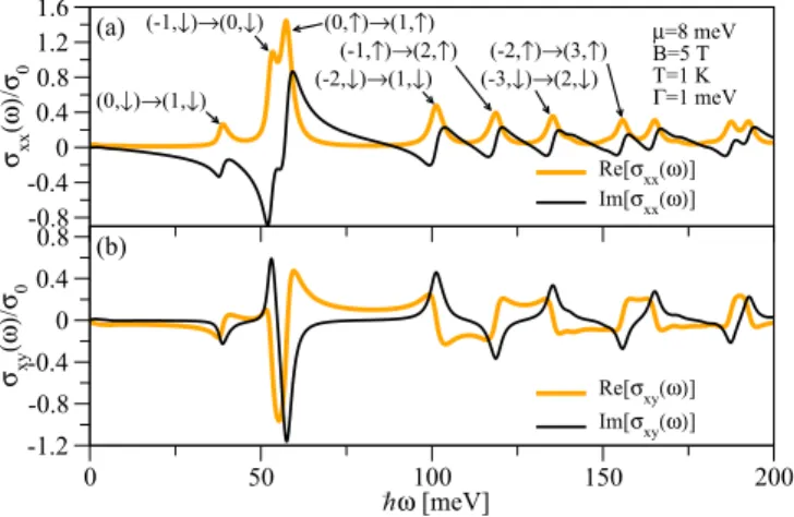
FIG. 3. (Color online) Real and imaginary parts of the (a) lon- gitudinal magneto-optical and (b) optical Hall conductivitiesσxx(ω) andσxy(ω) in a bulk HgTe QW of thicknessd=7.0 nm with some transitions explicitly labeled.
Calculating the dipole matrix elements dnnl,s(0,k) from the corresponding eigenstates yields the optical selection rules
|n| → |n±1|, s→s, k→k (19) for transitions between LLs.
To illustrate the resulting absorption spectrum, Fig.3shows the real and imaginary parts of the numerically [76] obtained magneto-optical conductivitiesσxx(ω) andσxy(ω) for the ma- terial parametersA=364.5 meV nm,B= −686.0 meV nm2, C=0,D= −512.0 meV nm2,M= −10.0 meV,ge=22.7, andgh= −1.21, corresponding to a QW thicknessd =7.0 nm
> dc [5,10], that is, for parameters in the QSH regime (at B=0). The magnetic field is chosen to be B =5 T, that is, a magnetic field below Bc≈7.4 T for which the model still shows an inverted band structure (see Fig. 2), while the remaining parameters are chosen to be T =1 K, μ= 8 meV, and=1 meV. Moreover, we note that the remaining components of the conductivity tensor can be determined from σyy(ω)=σxx(ω) andσxy(ω)= −σyx(ω) for the bulk system considered in this section.
As can be seen in Figs. 3(a) and 3(b), there are mul- tiple peaks in the absorptive components Re[σxx(ω)] and Im[σxy(ω)] corresponding to transitions between an occupied and an unoccupied LL state where the selection rules (19) have to be satisfied. Here, both intraband transitions, that is, transitions between only conduction LLs or only valence LLs, at low energies and interband transitions, that is, transitions between valence and conduction LLs, at higher energies are possible.
Due to the nonlinear dependence of the LLs (14)–(17) on n, different allowed transitions between LLs have different energies resulting in the multiple absorption peaks shown in Fig. 3(a) [68]. This behavior, also observed experimen- tally [62] and reminiscent of the situation in graphene [77–80], differs markedly from the behavior in a normal 2D electron gas, where equidistant LLs lead to only one absorption peak.
Moreover, we find that, while every transition satisfying
0 0.5 1 1.5
T=1 K T=100 K T=300 K
0 0.5 1 1.5
Re[σxx(ω)]/σ0
μ=8 meV μ=20 meV μ=50 meV
0 50 100 150 200
h_ω [meV]
0.01 0.1 1
10 B=0.1 T
B=1 T B=10 T
(a)
(b)
(c)
B=5 T μ=10 meV Γ=1 meV
T=1 K B=5 T Γ=1 meV
T=1 K μ=100 meV Γ=1 meV
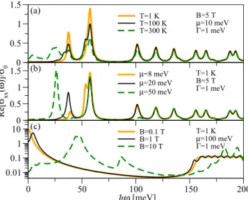
FIG. 4. (Color online) Real part of the longitudinal magneto- optical conductivityσxx(ω) in a bulk HgTe QW of thicknessd= 7.0 nm for different (a) temperaturesT, (b) chemical potentialsμ, and (c) magnetic fieldsB.
Eq. (19) occurs, different transitions are most probable for spin-up and spin-down LLs: If n1, the squared dipole matrix element for a transition−n→n+1 is typically five to ten times larger than the one of −n→n−1 for spin-up LLs and vice versa for spin-down LLs. Consequently, the prominent interband transition peaks are governed by−n→ n+1 for spin-up LLs and by −n→n−1 for spin-down LLs in Figs.3(a) and3(b), while other interband transitions contribute much less to the absorption spectrum.
In addition to the absorptive components, the refractive components Im[σxx(ω)] and Re[σxy(ω)] are also displayed for completeness. Both the absorptive and refractive components are generally needed to calculate optical observables, such as reflection coefficients and angles, for example.
In Fig.4, the dependence of Re[σxx(ω)] as a function of the frequency on different parameters is displayed for a bulk HgTe QW again in the QSH regime (at B =0). The temperature dependence is illustrated in Fig.4(a), which shows Re[σxx(ω)]
for a fixed magnetic field, chemical potential, and broadening.
Here, the main feature observed is that with increasing T additional (intraband) transitions (forbidden atT =0) become more probable which then give rise to new peaks—mainly at low frequencies. For higher frequencies, on the other hand, the magneto-optical conductivity remains largely unaffected, although the interband peaks are slightly reduced as spectral weight is transferred to lower energies, while the total spectral weight is conserved.
Figure4(b)shows Re[σxx(ω)] for several different chemical potentials and a fixed magnetic field, temperature, and broad- ening. Asμincreases, the intraband transition peaks move to lower energies, while the gap between intraband and interband transitions increases. Likewise, with decreasingB, the energy of the intraband transition peaks decreases and tends to zero, as can be seen in Fig.4(c), which displays Re[σxx(ω)] for several different values ofBand fixedμ,T, and.
The behavior of the intraband transition peaks with decreas- ing magnetic field or with increasing chemical potential can be qualitatively explained as originating from the LL spectrum in the vicinity of the Fermi level: For a fixed magnetic field, the LL spacing near the Fermi level decreases if the absolute value of the chemical potential is increased and thus situated in a denser region of the LL spectrum. Consequently, the energies of the intraband transitions are also decreased. On the other hand, with decreasing magnetic field the LL spacing decreases, giving rise to lower energies of the intraband transitions. Moreover, the amplitudes of the interband peaks decrease with decreasing magnetic fields, as seen in Fig.4(c).
This can be interpreted as arising from optical transitions between increasingly denser regions of the LL spectrum, where the energy difference between different transitions is small compared to the broadening due to scattering.
In the above discussion, we have investigated a QW with parameters corresponding to the topological regime (at B=0). However, the above conclusions on the behavior of the magneto-optical conductivity also apply to QWs with a thickness d < dc, that is, QWs in the topologically trivial regime. We conclude our discussion of bulk HgTe QWs by investigating also the spin magneto-optical conductivity σxxdiff(ω), where one can indeed find a signature of the transition between the QSH and the QH regimes: As shown in Fig.2, the transition between the QSH regime at finite magnetic field and the QH regime in QWs with a thicknessd > dc occurs when the spin-up and spin-down zero LLs cross at a critical magnetic fieldBc.
If the sample is undoped as chosen in Fig.5(a), the chemical potential lies between the two zero LLs. This, however, means that for B=Bc the chemical potential will lie in the two degenerate zero LLs. Thus, there is an additional Drude transition peak at zero frequency as shown in Fig. 5(a).
This peak originates from two different transitions, namely, spin-conserving transitions within the spin-up or spin-down
-0.5 0 0.5 1 1.5
Re[σxx(ω)]/σ0
Re[σxx(ω)]
Re[σdiffxx(ω)]
0 50 100 150 200
h_ω [meV]
-1 -0.5 0 0.5 1
(a)
(b)
μ=8.3 meV B=7.4 T T=1 K Γ=1 meV
μ=2.4 meV B=5 T T=1 K Γ=1 meV Drude peak
FIG. 5. (Color online) Real parts of the longitudinal and spin longitudinal magneto-optical conductivities, σxx(ω) and σxxdiff(ω), respectively, in a bulk HgTe QW of thicknessd=7.0 nm (a) at the critical magnetic fieldB=Bc≈7.4 T and (b) atB=5 T. In panel (a),μis chosen to be at the energy of the degenerate spin-up and spin-down zero mode Landau levels, while in panel (b)μ is chosen to be at the energy of the spin-up zero mode Landau levels.
zero LLs. As the squared dipole matrix elements for transitions within the spin-up and spin-down zero LLs are the same, both transitions contribute equally to the absorption peak atω=0.
However, this means that there is no peak atω=0 for the spin conductivityσxxdiff(ω) as spin-up and spin-down transitions cancel each other exactly.
This only happens at the critical field Bc in an undoped sample and is different from the situation ifμin a doped sample crosses one LL, an example of which is shown in Fig.5(b)for comparison. In this case, there is also a Drude peak atω=0 forσxx(ω), but since this peak arises from transitions within only one LL with a given spin quantum number,σxxdiff(ω) also exhibits a peak at zero frequency and can thus be distinguished from the peak arising from the two zero LLs atBc.
IV. FINITE STRIP
While in the previous section we have investigated the magneto-optical properties of bulk HgTe QWs without SOC, which did not account for the presence of edge states and where we did not find significant differences between the QSH and the QH regimes, we will now turn to a finite-strip geometry described by the confining potential in Eq. (5). Since the finite-strip geometry contains boundaries, both chiral QH edge states as well as helical QSH edge states emerge at these boundaries under the appropriate conditions: If the widthwof the finite wire is large compared tolB, well-localized QH edge states form in addition to the bulk LLs. In the QSH regime, that is, in a QW withd > dcand belowBc, there are also QSH edge states in addition to the QH states.
0.5 1 1.5
0.5 1 1.5
Re[σαβ(ω)]/σ0
0 50 100 150 200
h_ω [meV]
0 0.5 1 1.5
-1 -0.5 0 0.5
k [1/nm]
50 0 50 100
E [meV]
-1 -0.5 0 0.5
k [1/nm]
50 0 50 100
E [meV]
-2 -1 0 1
k [1/nm]
50 0 50 100
E [meV]
(a)
(b)
(c) 0
0
B=5 T d<dc μ=3 meV
B=5 T d>dc μ=8 meV
B=10 T d>dc μ=11 meV
Drude peak
FIG. 6. (Color online) Real parts of the longitudinal magneto- optical conductivities σxx(ω) and σyy(ω) in (a) a HgTe QW of thickness d=5.5 nm and with a magnetic field B=5 T, (b) a HgTe QW withd=7.0 nm andB=5 T, and (c) a HgTe QW with d=7.0 nm andB=10 T. Here, spin-orbit coupling corrections are not included. The solid orange lines representσxx(ω)=σyy(ω) in a bulk system, while the solid black and the dashed green lines represent σxx(ω) andσyy(ω) in a finite strip of widthw=200 nm. The insets in panels (a)–(c) illustrate the respective energy spectra of the finite strip and the positions of the chemical potential (dotted lines).
This can also be seen in Fig.6, which shows the real parts of the magneto-optical conductivitiesσxx(ω) andσyy(ω) for a finite strip of widthw=200 nm for different QW thicknesses and magnetic fields corresponding to different regimes [81]
without SOC (0=0 andξe=0): a QW withd < dc, that is, a system with no QSH states at any magnetic field [Fig.6(a)];
a QW withd > dcandB < Bc, that is, a system possessing QSH states at the edges of the strip [Fig.6(b)]; and a QW withd > dc, butB > Bc, that is, a system with no QSH states [Fig.6(c)]. For each of the regimes, we have chosenμto lie at the neutrality point between the uppermost valence LL and the lowest conduction LL. The insets of Figs.6(a)–6(c) show the respective energy spectra and the positions ofμ.
In the regimes without any QSH edge states [Figs.6(a) and6(c)], the band structure is gapped as every electronlike LL is a conduction band and situated above the holelike valence bands. The edge states associated with an electronlike LL have positive curvature, while those associated with a holelike LL have negative curvature [82]. Figure6(b), on the other hand, shows a different situation as the lowest electronlike (spin-up) LL is a valence band and the highest holelike (spin-down) LL is a conduction band. Thus, there is a crossover between the dispersions of electron- and holelike bands and one consequently finds counterpropagating spin-polarized QSH states, in addition to QH edge states propagating in the same direction at a given boundary regardless of spin. For comparison, the magneto-optical conductivities for a bulk HgTe QW as investigated in Sec. III are also displayed in Fig.6for the same magnetic fields and QW thicknessesd as the finite-strip structures.
Compared to the situation in a bulk HgTe QW, we can see that in a finite strip there are still pronounced absorption peaks arising from the bulk LLs. However, the spectral weight of these peaks is reduced as transitions between edge states are also possible. Since the energy of these transitions can differ from the energy difference between two bulk LLs and the total spectral weight is conserved, some spectral weight is transferred from the peaks to the regions between the absorption peaks, a phenomenon clearly seen in Fig.6.
A second difference compared to the bulk system is that, even if the chemical potential is not situated in a bulk LL, there is a Drude-like absorption peak at low energies forσxx(ω).
Analogous to the situation in Fig.5, where a Drude peak at low energies originated from transitions within bulk LL states though, this absorption peak arises from transitions that occur when the energy of a QH or QSH edge state is at the chemical potential or close to it (within the broadening). This mechanism is present in both the QH and QSH regimes if the chemical potential is above or below the bulk band gap. The difference between those two regimes, however, is that edge states exist at every energy in the QSH regime, while there are no states with energies inside the bulk gap in the QH regime (see the insets in Fig.6). Hence, if in the QH regime the chemical potential lies inside the gap and the gap exceeds the energy scale associated with broadening, no low-energy absorption peak occurs as seen in Figs.6(a)and6(c). Moreover, we note that this Drude peak appears only along the unconfined direction, but not forσyy(ω) along the confined direction. This is to be expected because only thex direction is associated with free acceleration.
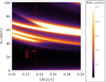
FIG. 7. (Color online) Real part of the total longitudinal magneto-optical conductivity σxx(ω) of a finite strip with width w=200 nm, =1 meV, and chemical potentialμ=8 meV at temperatureT =1 K as a function of the inverse magnetic field 1/B andωfor band parameters corresponding to a HgTe QW of thickness d=7.0 nm without spin-orbit coupling corrections. The vertical line indicates the inverse critical magnetic field separating the QSH and QH regimes and as calculated by Eq. (18).
The disappearance of the Drude peak ifμremains inside the bulk gap during the transition from the QSH to the QH regime is also illustrated in Fig. 7: Here, the absorption spectrum of a finite-strip geometry for a QW withd=7.0 nm
> dc (and without SOC) is shown as a function of 1/B and ω at low temperatures and fixed chemical potential. For 1/B=0.2/T, the situation is described by Fig.6(b). As 1/Bis decreased, that is, as the magnetic field is increased, the absolute value of the LL energies and thus the photon energies of their associated absorption peaks increase. At low photon energies, there is a finite absorption, which vanishes for magnetic fields above the critical fieldBcwhen the transition from the QSH into the QH regime occurs.
We now address the effect of SOC. While the states in Fig.6 have been perfectly spin polarized and characterized by the spin quantum numbers, the situation changes if SOC is considered, that is, if 0 and/or ξe are finite in the total Hamiltonian (3). This is illustrated in Fig. 8, where the real parts of the magneto-optical conductivitiesσxx(ω) andσyy(ω) are displayed for a QW of thickness d =7.0 nm > dc at B=5 T (see above) with the additional SOC parameters 0=1.6 meV and ξe=16.0 meV nm [11]. The inset of Fig. 8 compares the energy spectrum near the band gap in the presence of SOC with the spin-polarized energy spectrum in the absence of SOC. The most striking effect appears at the crossing between the spin-up and spin-down states, where a SOC gap is opened up. Consequently, the low-energy absorption peak present in the QSH regime without SOC is reduced if the chemical potential is situated inside this small gap. However, as long as the gap opened by SOC does not significantly exceed the broadening, an increased absorption for σxx(ω) can still be observed in the QSH regime at low photon energies ω. As bands farther away from the zero
0 50 100 150 200
h_ω [meV]
0 0.25 0.5 0.75 1 1.25
Re[σαβ(ω)]/σ0
σxx (without SOC) σxx (with SOC) σyy (with SOC)
-1 -0.5 0 0.5
k [1/nm]
0 5 10 15
E [meV]
with SOC T=1 K
μ=8 meV B=5 T d>dc Γ=1 meV
SOC
SOC gap
FIG. 8. (Color online) Real parts of the longitudinal magneto- optical conductivitiesσxx(ω) andσyy(ω) of a finite strip with width w=200 nm, a magnetic field B=5 T, and band parameters corresponding to a HgTe QW of thickness d=7.0 nm with and without spin-orbit coupling corrections as given in Eq. (3). The respective energy spectra and the position of the chemical potential (dotted line) are shown in the inset.
LLs are affected even less by SOC for the parameters given above, the absorption spectrum at higher energies remains nearly unaltered compared to spin-polarized case.
Next, we turn our attention to the effect of temperature on the absorption spectrum in general and on the Drude-like peak arising from QSH states in particular and compare this to the QH regime. For this purpose, Figs. 9(a) and 9(b) show Re[σxx(ω)] in a finite-strip geometry (without SOC) at different temperatures for a QW with d =7.0 nm > dc in the QSH and QH regimes, respectively, with the chemical potential situated between the zero LLs. Complementary,
0 0.5 1 1.5
2 T=1 K
T=100 K T=300 K
-1 -0.5 0 0.5
k [1/nm]
100 50 0 -50
E [meV]
0 50 100 150 200
h_ω [meV]
0 0.5 1 1.5 Re[σxx(ω)]/σ0
-2 -1 0 1
k [1/nm]
100 50 0 -50
E [meV]
μ=8 meV B=5 T d>dc
Γ=1 meV
(a)
(b)
μ=11 meV B=10 T d>dc Γ=1 meV
(0,↑)→(1,↑) (-1,↓)→(0,↓)
FIG. 9. (Color online) Real part of the longitudinal magneto- optical conductivityσxx(ω) of a finite strip with widthw=200 nm, band parameters corresponding to a HgTe QW of thicknessd= 7.0 nm without spin-orbit coupling corrections, and magnetic fields of (a)B=5 T and (b) B=10 T for different temperatures T. The energy spectra and the positions of the chemical potential (dotted lines) are shown in the insets.
FIG. 10. (Color online) Real part of the total longitudinal magneto-optical conductivity σxx(ω) of a finite strip with width w=200 nm as a function of the temperatureT andωforB=5 T, μ=8 meV, =1 meV, and band parameters corresponding to a HgTe QW of thicknessd=7.0 nm without spin-orbit coupling corrections.
Fig. 10 displays Re[σxx(ω)] for the setup of Fig.9(a) as a function ofT andω.
Similar to the situation in a bulk QW illustrated in Fig.4(a), additional transitions especially, but not exclusively, at low energies become more probable. This results in additional absorption peaks and an increase of the absorption at low energies, while spectral weight is transferred away from the intraband peaks as can be seen in Figs. 9 and 10. Since the spin-up and spin-down zero modes are very close to μ in these setups, additional transitions involving one of these LLs become especially likely if T is increased and consequently the LL below μis depopulated, while the LL aboveμis populated. This is particularly striking in Fig.9(b), where already atT =100 K pronounced peaks appear due to transitionsn=0→1 and−1→0 for spin-up and spin-down LLs, respectively.
As the absorption at low energies becomes more probable, an enhancement of the low-energy absorption peak in the QSH regime can be observed in Figs. 9(a) and10. On the other hand, Fig.9(b)shows that such a peak also appears in the QH regime with increasing temperature. The smaller the gap between conduction and valence LLs, the smaller is the temperature for the onset of this effect. Thus, at highT both regimes exhibit a low-energy absorption peak forσxx(ω).
This is also corroborated by Fig.11(a), where the real part ofσxx(ω) at low energies is displayed as a function ofT for a QW in the QSH regime, in the QSH regime with SOC, and in the QH regime with the chemical potential situated between the conduction and valence LLs. At low temperatures, there is a finite absorption in the QSH regime, even if reduced by SOC, whereas there is no absorption in the QH regime.
With increasing T, the absorption also increases, in both the QSH and QH regimes, although the increase is more pronounced in the QSH regime. Moreover, SOC corrections are less pronounced at higher temperatures. Without SOC, a
0.2 0.4 0.6
Re[σxx(ω0)]/σ0
0
B=5 T, μ=8 meV, d>dc
B=5 T, μ=8 meV, d>dc (SOC) B=10 T, μ=11 meV, d>dc
0 50 100 150 200 250 300
T [K]
0 0.1
Re[σdiff xx(ω0)]/σ00.15 (a)
(b) Γ=1 meV h_
ω0=0.1 meV
FIG. 11. (Color online) Real parts of the (a) total and (b) spin longitudinal magneto-optical conductivitiesσxx(ω) andσxxdiff(ω) of a finite strip with widthw=200 nm at low frequenciesω0as a function of the temperatureT for different setups.
spin conductivityσxxdiff(ω) can be defined, whose temperature dependence is shown in Fig.11(b) and closely follows the temperature dependence ofσxx(ω).
Finally, we study the dependence of the low-energy ab- sorption on the chemical potential. For this purpose, Fig.12(a) shows the real parts of the conductivity σxx(ω) at low ω and T as functions of μ for a QW in the QSH regime, in the QSH regime with SOC, and in the QH regime. The corresponding spin conductivities σxxdiff(ω) for the regimes without SOC are displayed in Fig.12(b). As can be seen in Fig. 12(a), the absorption in the QSH regime is finite and usually higher than in the QH regime. Spin-orbit coupling in the QSH regime only has a significant effect close to the crossing between the electron- and holelike edge dispersions, that is, in the energy interval approximately between 5 and 15 meV. In this region,σxx(ω) is reduced due to SOC, although it does not vanish completely. The behavior with varying chemical potential in the QH regime, on the other hand, is different: If μ is situated in the gap between the valence
0.2 0.4 0.6 0.8
Re[σxx(ω0)]/σ0
0
B=5 T, d>dc
B=5 T, d>dc (SOC) B=10 T, d>dc
0 5 10 15 20
μ [meV]
-0.2 0 0.2 0.4 0.6
Re[σdiff xx(ω0)]/σ00.8 (a)
(b)
T=1 K Γ=1 meV h_ω0=0.1 meV
FIG. 12. (Color online) Real parts of the (a) total and (b) spin longitudinal magneto-optical conductivitiesσxx(ω) andσxxdiff(ω), re- spectively, of a finite strip with widthw=200 nm at low frequencies ω0as a function of the chemical potentialμfor different setups.
FIG. 13. (Color online) Real part of the total longitudinal magneto-optical conductivity σxx(ω) of a finite strip with width w=200 nm and=1 meV at low energiesω0=0.1 meV and temperatureT =1 K as a function of the chemical potentialμand magnetic fieldBfor band parameters corresponding to a HgTe QW of thicknessd=7.0 nm without spin-orbit coupling corrections. The vertical line indicates the critical magnetic field separating the QSH and QH regimes and as calculated by Eq. (18).
and conduction LLs, there is no Drude-like peak andσxx(ω) vanishes.
Thus, by sweeping the gate voltage and thereby varying the position of the chemical potential, it is possible to distinguish between the QSH and QH regimes on the basis of their their low-energy absorption as depicted in Fig.12(a). We note that this behavior of the Drude peak in the absorption spectrum is consistent with and reflects the expected behavior of the dc conductance in the QSH and QH regimes [3].
This is also substantiated in Fig. 13, which shows the low-energy absorption of a QW of thickness d=7.0 nm without SOC corrections as a function of both the chemical potential as well as the magnetic field. While in the QSH regime,B < Bc≈7.4 T, Re[σxx(ω)] never vanishes entirely, there is a region where Re[σxx(ω)] is completely suppressed in the QH regime above Bc. With increasing magnetic field, the extent of this region grows as the gap between conduction and valence LLs increases. Outside the region of suppressed conductance and low-energy absorption, the spectrum displays an oscillatory behavior as seen in Figs.12 and13.
Finally, we remark that our description does not take into account many-body effects, such as (edge) magneto-plasmon resonances which can potentially play a prominent role for the absorption especially in narrow strips [83–85]. Since the scheme that we propose to distinguish between the QSH and QH regimes is based on the dc conductivity, however, we think this scheme to be robust, even in the presence of edge magneto-plasmons, although the absorption at low but finite energies can obtain a richer structure than the single-particle absorption calculated in this paper. Moreover,
our single-particle calculations provide a useful benchmark against which to test experimental results.
V. CONCLUSIONS
Inverted HgTe/CdTe QWs exhibit helical QSH states below a critical magnetic fieldBc, above which the band order is normal and only QH states can be found. In this work, we have studied the magneto-optical properties of such HgTe/CdTe QWs by calculating the magneto-optical conductivity using linear-response theory. We have considered both an infinite 2D system as well as a finite strip, that is, a 2D system that is confined in one direction. The normal and the inverted regimes both exhibit a series of pronounced absorption peaks corresponding to different transitions, both intraband as well as interband transitions, between nonequidistant LLs in the infinite system. Thus, it is hard to distinguish between the QSH and QH regimes based on these LL peaks.
We find that these bulk LL peaks also occur in the finite strip, where the presence of edge states results in an additional Drude-like absorption peak inσxx(ω) originating from low-energy transitions at the Fermi level. This Drude peak is always present in the QSH regime, while it vanishes in the QH regime if the chemical potential is situated in the bulk gap. If SOC corrections are included, we find that their effect is to open up a small gap in the QSH spectrum, which leads to a reduction but not to a complete disappearance of this Drude peak. By sweeping the gate voltage of a finite QW structure and thereby varying the position of the chemical potential, it is therefore possible to experimentally distinguish between the QSH and QH regimes on the basis of the stability (QSH) or disappearance (QH) of the Drude peak.
ACKNOWLEDGMENTS
This work was supported by Deutsche Forschungsge- meinschaft Grants No. SCHA 1899/1-1 (B.S.) and No. SFB 689 (J.F.); U.S. ONR Grant No. N000141310754 (B.S. and A.M.-A.); U.S. Department of Energy, Office of Science Basic Energy Sciences, under Award No. DE-SC0004890 (I. ˇZ.);
as well as the International Doctorate Program Topological Insulators of the Elite Network of Bavaria (J.F.).
APPENDIX A: EIGENSPECTRUM AND EIGENSTATES 1. No spin-orbit coupling corrections
Inserting the ansatz from Eq. (7) in the Schr¨odinger equation given by the Hamiltonian (6) for0=ξe=0 and introducing the transformation
ζ =ζ(y)=√ 2
y−lB2k
lB (A1)
yields a system of two differential equations to determine the eigenenergyE=ns(k) and eigenstates with given spin and

![Fig. 10 displays Re[σ xx (ω)] for the setup of Fig. 9(a) as a function of T and ω.](https://thumb-eu.123doks.com/thumbv2/1library_info/5585991.1690528/8.911.77.443.103.395/fig-displays-σ-xx-ω-setup-fig-function.webp)
