Institute for Theoretical Physics

(1)

Institute for Theoretical Physics

University of Cologne

Bachelor Thesis

The influence of backwards mutations on the number of accessible paths in a fitness landscape

Written by Mario Josupeit

Supervisor: Prof. Joachim Krug

Cologne, 21st of December 2015

(2)

(3)

1 Introduction

Ever since the days of Darwin people have pondered how evolution created all organisms the way they are today. This idea can be taken further though as we are now trying to understand how the same organisms will evolve in the future. Learning about how evolution works and what direction it will take is naturally one of the most interesting things a person can think about since it is one of the few if not one of the only ways we can predict a complicated future in simple scientific manners.

1.1 The goal of this thesis

This thesis will be about trying to find out which paths evolution took for some selected small organisms and about the influence of backward mutations on a genetic landscape.

We will take a look at empirical data and also find features of the models that we use to understand them. Therefore it is important to know about epistasis, which we will treat here as the influence of one mutation on the effect of another. This definition is different from a lot of other definitions that exist for this term (see also [1]).

1.2 The concept of heredity

Important in this context is the concept of genetic alleles. We will assume that the features in question will be passed on to the next generation via alleles during asexual reproduction which can be altered by mutation and also altered backwards into the original state. This alteration replicates for example the expression or repression of genes which can lead to the activation or inactivation of proteins and thus determines the features and abilities of the organism.

1.3 Hypercubes and accessible paths

If we now consider an organism in a certain state, we can think of every feature or allele as a binary digit also called locus with two values {0,1}. If we are talking aboutLloci, every genetically different individual is located somewhere on the {0,1}^Lhypercube. In this case, mutations are equivalent to moving from one point on the hypercube to another. Every point of the hypercube can thereby be considered a vector p~∈{0,1}^L. For understanding hypercubes see [2] and how they can be a model for a genetic landscape see [3].

(5)

1.4 The House of cards model These vectors can now be assigned a fitness value, which can be considered as the expected number of offspring of one individual with respect to their environment. So if there are two species with different fitness values in a population with constant size the population will fix towards the one with the higher fitness. Fixing means for the organisms that the whole population is replaced by the better adapted individuals, which are the ones who produce more offspring and will eventually crowd out the other one. The time this process takes is called fixation time and it is defined by Kimura in [4].

In nature mutations which are not null mutations are not frequent. These mutations change the product the genes are coding for. So it is safe to assume that if we keep the size of the population constant and also do not change the environmental conditions from when we started we can assume a large time between mutations compared to the fixation time, meaning the new and better species has already taken over the population by the time the next mutation happens. The model describing this assumption is called the strong selection weak mutation model (SSWM) as described by Gillespie [5].

If we consider multiple mutations that happen one after the other we can assume paths on the hypercube with step length = 1 because we use the SSWM model and go from points with lower fitness to points with higher fitness. In the end we will reach a local or the global maximum, both of which are the best adapted version of the organism with respect to the environmental conditions in its neighborhood. The neighborhood describes all versions of the organism which are just one mutation away. If we started opposite of the global maximum, the length of the paths to the global maximum will at least be equal to the dimension L.

1.4 The House of cards model

For the numerical analysis of the paths in this thesis I will use the house-of-cards (HoC) model introduced by Kingman [6]. This model treats the different genotypes as completely independent which results in a hypercube that has random fitness values at each site and a global maximum at the end point. This means here that the fitness values are uniformly distributed ∈ (0,1) and equal to 1 at the point (1,1, . . . ,1). The start value can either be fixed to a number x ∈ (0,1) or random as well. The random number generator uses a "Mersenne Twister"-algorithm to keep correlations between the random numbers to a minimum and to have an acceptable calculation time.

(6)

1.6 Number of paths on the hypercube

1.5 The Rough Mt. Fuji model

As we will see later it will be necessary to use a more general model for fitness landscapes and do the same calculations with this one. We use the rough Mt. Fuji model, which adds a gradient to the random numbers of the HoC model. This means, depending on the distance from the origin to the sites on the hypercube we get fitness values given by:

f(~σ) = c|~0−~σ|+f_HoC(~σ) (1.5.1) This gives a landscape tunable with c. A larger value ofcreduces ruggedness of the landscape and c = 0 gives a limit which is a landscape equal to a HoC one. For this model mutations do not only have a random value for their outcome but also a gradually increasing component so it is a intermediate model between a smooth and a random landscape.

This model was introduced by Aita in 2000 [12].

1.6 Number of paths on the hypercube

There are different kinds of paths on the hypercube. The directed paths take the shortest route to the global maximum from its antipodal point. They are also called short orp=0.

Paths that take a longer route are called long paths or p>0. p is the number of reversions along this path. A reversion undoes a previously taken step, it is a step "backwards" in the direction of a previous one so to speak. If a reversion appears, the total length of the path grows by two because this extra step makes the path to the end point one step longer, which adds up to a contribution to the total length of 2. It is obvious that there are L!

directed paths, which means that p= 0, from (0,0, . . . ,0) to (1,1, . . . ,1) on theH_L². "H_L²"

is the hypercube of dimension L and edge length 1. If one of these paths is accessible the L values on the sites of this path have to be in ascending order. The probability to have such a setup is _L!¹. This means that the expected number of accessible paths of length L is E = 1 in all dimensions [8]. If there are fixed starting values, L−1 values have to be ordered in a certain way, with the probability to be larger than xbeingP(X > x) = 1−x.

x is the fixed value of the start point.

E^x = L

L−1

!

(1−x)^L−1 =L(1−x)^L−1 (1.6.2)

(7)

1.6 Number of paths on the hypercube We can see the threshold in x. If x is larger than ^ln(L)_L the E^x will go to infinity for L going to infinity, ifxis smaller than this value, the expected value will go to 0 for the same limit. Whenever we have backwards mutations, there will be more possible paths. The total number of non-intersecting paths will be called a_L,p here which can not be calculated for all values of L and p, but which can be obtained by counting all the paths so to speak by hand using brute force calculation. This means for a certain p and x, that:

E_p^x =aL,p

(1−x)^L+2p−1

(L+ 2p−1)! (1.6.3)

For all p combined one has to sum over p:

E^x =^X

p≥0

aL,p

(1−x)^L+2p−1

(L+ 2p−1)! (1.6.4)

If one now wants to find how many paths there are with a random start value one has to integrate over all xin (0,1):

Z 1 0

dxE^x(Θ) =

−^X

p≥0

a_L,p(1−x)^L+2p (L+ 2p)!

x=1 x=0

=^X

p≥0

a_L,p

(L+ 2p)! (1.6.5) For comparing the numerical curves to these analytical ones one can approximate the sum by its terms up to the 2nd order because (L+ 2p−1)!a_L,p for larger p. The coefficients a_L,p can be calculated up to second order in p with:

a_L,0 =L! (1.6.6)

a_L,1 =L!L(L−1)(L−2)

6 (1.6.7)

a_L,2 =L!(L−1)(L−2)(5L⁴+ 3L³+ 34L²−264L+ 180)

360 (1.6.8)

These derivations have been done by Berestycki et al. [10]. The brute force calculated values for L= 5 from the same paper are:

a5,0 = 5!, a_5,1 = 5!·10, a_5,2 = 5!·107, a_5,3 = 5!·1097, a_5,4 = 5!·9754, a_5,5 = 5!·72305, a_5,6 = 5!·448536, a_5,7 = 5!·2243671, a_5,8 = 5!·8631118, a_5,9 = 5!·24044702, a_5,10= 5!·44617008, a_5,11 = 5!·48280086, a_5,12 = 5!·24000420, a_5,13 = 5!·3080792.

(8)

1.7 The implications for real organisms

To connect the theoretical results to real life experiments some of the fitness landscapes also used in the paper by Szendro et al.[11] were put into the algorithm to figure out which implications can be drawn here. Something that is interesting here is the number of paths with respect to their length. The idea for this analysis came from the discussion of Weinreich’s data [7] in the paper by De Pristo [9]. Its aim was the description of all possible paths on an empirical landscape.

For the large landscapes we can also create substructures of the hypercubes given, which are hypercubes of lower dimensions themselves. We will call them subcubes and analyze them in terms of accessible paths. In this thesis we will also get ensembles of smaller graphs contained in larger ones and obtain information about the larger one by looking at the Subcubes, defined in 2.3, like Szendro et al. did in their paper.

(9)

2 Algorithms

For the simulation there are different versions of the program. One version will generate multiple hypercubes of a given dimension (section 2.1) with either the HoC model or the Mt. Fuji model and the other will find paths on hypercubes of given data (section 2.2) or find subcubes (defined in 1.7) and analyze them. The searching algorithm is mostly the same in both cases. The latter version takes a hypercube of dimension L and creates lower dimension subcubes which can then be analyzed to obtain an ensemble of hypercubes which are indicative of ruggedness and other features of the hypercube of dimension L.

2.1 Numerical analysis version

2.1.1 House of Cards variant

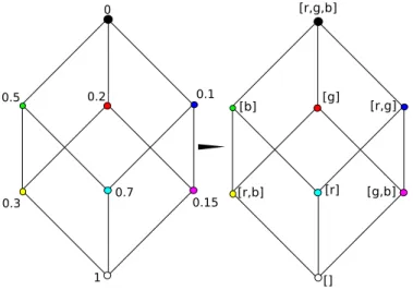
The algorithm starts by generating 2^L uniform random numbers drawn from (0,1), which are associated with the points on a hypercube.

Then the value at site (1,1, . . . ,1) is associated with the value 1. It now proceeds by comparing the fitness values of each site to the neighboring ones. If the value of the neighboring site is higher, the direction the neighbor is in is written into an array associated with the current site.

0

0.5 0.2 0.1

0.3 0.7 0.15

1

[r,g,b]

[g] [r,g]

[g,b]

[r,b]

[b]

[r]

[]

Figure 2.1.1: The same H₃² in two realizations. Left: with fitness values. Right: with possible directions from each corner. The characters in the brackets are acronyms of the possible "color-directions". - or& are blue, % or. are green,↑ or ↓ are red.

This will transform the hypercube of fitness values into one of accessible directions. Now the algorithm starts at (0,0, . . . ,0) in theH_L² hypercube and recursively takes steps in the

(10)

2.2 Empirical landscape analysis

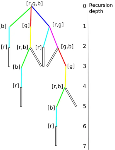
allowed directions. This can be represented by a graph in a "tree" shape whose branches describe the possible paths.

[r,g,b]

[b]

[r]

[g]

[r,b]

[g,b]

[r,g]

[r,b]

Recursion depth 0 1

2 3

4 5 6

7

Figure 2.1.2: "Tree" of accessible paths. Colored lines represent the paths to the colored dots in the cube2.1.1. As one can see, there are 4 paths with path length L, 2 with L+ 2 and 1 with L+ 4

The recursion depth is then equivalent to the length of the accessed path. If it reaches the (1,1, . . . ,1) point, it adds 1 to the number of paths with the length it currently has and this way produces a distribution of path numbers sorted by length. In the example H₃² this would be [4,2,1]

2.1.2 Rough Mt. Fuji variant

On top of the random values of the house of cards model, a linear function of the distance to the origin is added to the fitness values as described before. This results in new fitness values given by (1.5.1).

2.2 Empirical landscape analysis

For analyzing the empirical data, the algorithm reads out the given file, counts the lines (cl) and creates a dictionary that assigns the given fitness values to their coordinates. It also

(11)

2.3 Subcube analysis finds the maximum of the H_L² hypercube where L is calculated as L = ^ln(cl)_ln(2) and saves it as the end point. Then the cube is transformed like in section 2.1. It then starts opposite to theend point of the hypercube and finds the distribution of paths with respect to their length, just like in version 2.1.

2.3 Subcube analysis

Subcubes can be obtained by fixing n of the L lines of coordinates to either 1 or 0. This means that one obtains s_L,n.

s_L,n= 2ⁿ L n

!

(2.3.1) s_L,n is the number of subcubes of dimension L− n from a hypercube of dimension L.

Then the ensemble of subcubes is put into a loop which calculates the distribution of path numbers with respect to path length like in 2.1 and 2.2.

(12)

3 Numerical results

In this chapter we take a look at the results of the program described in 2.1.

3.1 Comparing results

To correctly evaluate the results of the algorithm, it is necessary to compare some results to existing ones. This does not only test whether or not the algorithm works as intended but also gives insight into its limitations. If we use the algorithm described before in the following calculations, lots of details are neglected but still calculated, meaning that espe- cially with higher dimensions the process takes quite a long time. Therefore there are no comparisons for dimensions larger than 15.

3.1.1 House-of-cards model with fixed start values

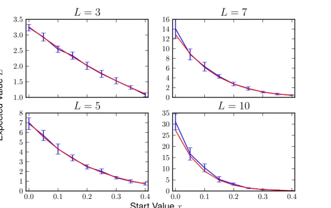
For evaluating the HoC model with fixed start values, we has to take into account that the numerical results should usually be larger than the analytical ones since the sum in formula (1.6.4) is approximated by the first three terms for all cases except forL= 3, where the sum has 3 terms in total andL= 5 where alla_L,pare given in section1.6. All terms are positive so the approximation should have a lower value than the numeric value. The numerical results have been averaged over 10⁴ hypercubes in each dimension. As an example these are the results for dimensions L∈ {3,5,7,10} and start values x∈ {0,0.05, . . . ,0.4}:

As expected the curves in figure 3.1.1 closely match each other. The blue curve is most of the time larger than the red one.

(13)

3.1 Comparing results

1.0 1.5 2.0 2.5 3.0

3.5

L = 3

0 2 4 6 8 10 12 14

16

L = 7

0.0 0.1 0.2 0.3 0.4

0 1 2 3 4 5 6 7

8

L = 5

0.0 0.1 0.2 0.3 0.4

0 5 10 15 20 25 30

35

L = 10

Start Valuex

ExpectedValueE

Figure 3.1.1: The numerical curve (blue) and the one calculated with the formula (red) are plotted here with errors for the numerical results

3.1.2 Probability to have at least one open path

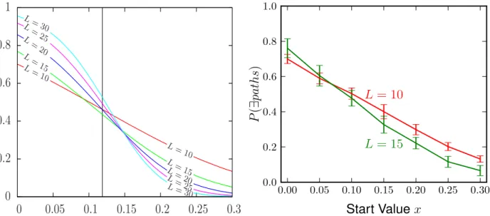
In the same paper by Berestycki et al. [10] they also calculate the probability that a hypercube would have at least one path from the start to the end point, while looking at different dimensions and also at different start values. As mentioned before, the algorithm used for this thesis can unfortunately not produce results in all dimensions they calculated because it collects a lot of detail information (e.g. all the paths) and the data volume was too much to handle for the computer that was used. But it is possible to make a comparison to their dimension ≤15 cases:

(14)

3.2 Directed vs arbitrary paths

L= 30 L= 25 L= 20 L= 15 L= 10 L= 30

L= 25 L= 20 L= 15 L= 10

0.3 0.25 0.2

0.15 0.1

0.05 0

1 0.8 0.6 0.4 0.2

0 ^0.0^0.00 ^0.05 ^0.10 ^0.15 ^0.20 ^0.25 ^0.30

0.2 0.4 0.6 0.8 1.0

L = 10

L = 15

Start Valuex

P(∃paths)

Figure 3.1.2: Left: the calculated curves in the image taken from of Berestycki et al. [10]

Right: The curve calculated with this thesis’ algorithm, where thegreencurve is dimension 15 averaged over 1000 cubes and thered one is dimension 10 averaged over 10⁴ cubes

As we can see the behavior for the 10⁴ runs for dimension 10 is close to linear just like in the graph on the left and the values do not deviate much from the other graph. The curve for dimension 15 looks much more crooked due to it being only the data of 1000 hypercubes but its propagation and values are very similar to the curve in the other graph.

The crossing point between both is close to the same point in both graphs as well.

3.2 Directed vs arbitrary paths

As the title of this thesis suggests, finding out about the total number of accessible paths to the fitness maximum is the main goal of this work. We can now take a look at either the distribution of the number of accessible paths of each length or the expected number of paths with regard to their dimension.

3.2.1 Expected number of paths

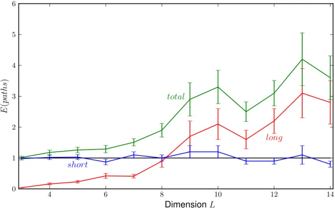
For these calculations, HoC-cubes with random start values were used. The number realizations in each dimensions was 5000.

(15)

4 6 8 10 12 14

0 1 2 3 4 5 6

long short

total

DimensionL

E(paths)

Figure 3.2.3: The numerically calculated expectation values

As we can see the graph of the number of short paths (p= 0) which is supposed to be close to 1 seems to be dented at the same dimensions as the graph of long (p >0) and also all paths (arbitraryp), since those are just the sum of short and long paths. This could mean that the number of paths of different lengths are correlated. Therefore we will try to give arguments for the normalization of the number of long/arbitrary paths by the number of short paths. This would mean that we will divide the number of long and arbitrary paths through the number of short paths to get smoother graphs.

To validate this normalization, it is important to figure out how strongly these values are correlated. Therefore the correlation between long (p > 0) or arbitrary and short paths (p= 0) was calculated. Here li/s_i/t_i is the number of long/short/arbitrary paths normed by their average of hypercube number i∈ {1, . . . ,5000} and c_l/c_t is the correlation value for the long/arbitrary paths. This should result in a measure for the likelihood of there being a lot of one type of path, given that there are already a lot of another type.

c_l = h(l_i− hl_ii)(s_i− hs_ii)i

qh(l_i − hl_ii)²ih(s_i− hs_ii)²i (3.2.1)

(16)

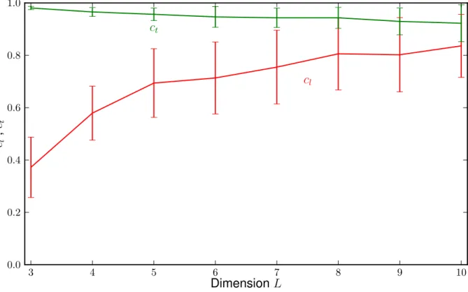
This results in the following graph of c_l(L) andc_t(L):

3 4 5 6 7 8 9 10

0.0 0.2 0.4 0.6 0.8 1.0

c_l c_t

total

DimensionL cl,ct

Figure 3.2.4: The graph shows cl in red and ct in green

Seeing that the correlation value is close to 1 for higher dimensions for the long paths and close to 1 for the arbitrary ones in all dimensions, we can assume that these values are correlated.

(17)

3.2 Directed vs arbitrary paths Another measure for correlation is to map the values on a XY graph. For some example dimensions long path numbers plotted on the y-axis against short path numbers on the x-axis look like this:

0.0 0.5 1.0 1.5 2.0 2.5 3.0 3.5 4.0 0

1 2 3 4 5 6

L= 6

y=x

ln(short path number)

ln(longpathnumber)

0 1 2 3 4 5

0 1 2 3 4 5 6 7

L= 12

y=x

ln(longpathnumber)

Figure 3.2.5: For dimension 6 & 12 these graphs show the long paths plotted against the number of short paths on a double logarithmic scale. The green line represents y=x.

c_t plotted in the same way:

0.0 0.5 1.0 1.5 2.0 2.5 3.0 3.5 4.0 0

1 2 3 4 5 6 7

L= 6

y=x

ln(totalpathnumber)

0 1 2 3 4 5

0 1 2 3 4 5 6 7

L= 12

y=x

ln(totalpathnumber)

Figure 3.2.6: For the same dimensions these graphs show the total number of accessible paths plotted against the number of short paths on a double logarithmic scale.

In these graphs we can see that there are large bulks of points right next to the lines markingx=yand much less in the upper left and lower right corner. From this image we can assume that there is in fact correlation between the short and long/arbitrary paths Knowing this, we can proceed as we suggested above by dividing the long and arbitrary number of paths through the number of short paths:

(18)

4 6 8 10 12 14

0 1 2 3 4 5 6

long short

total

DimensionL

E(paths)

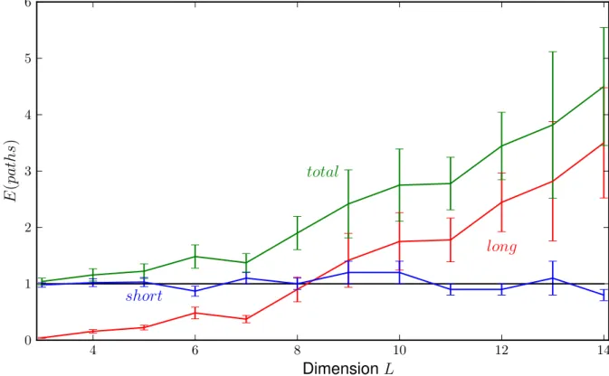
Figure 3.2.7: After dividing the number of long and total paths by the number of short the graphs look much smoother.

We will use the expected values later to compare them to the experimental data.

(19)

3.3 Rough Mt. Fuji expected values

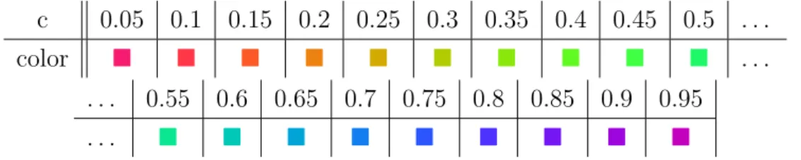
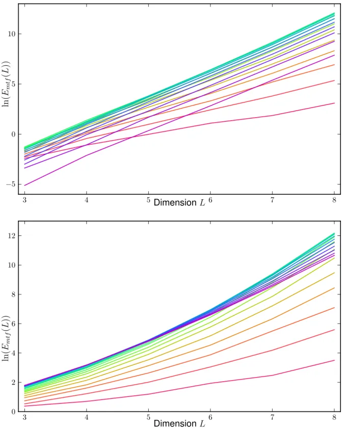
For later comparison we have to calculate the number of expected paths in the Mt. Fuji model as well. In the following the graphs will be color coded depending on the cused.

c 0.05 0.1 0.15 0.2 0.25 0.3 0.35 0.4 0.45 0.5 . . .

color . . .

. . . 0.55 0.6 0.65 0.7 0.75 0.8 0.85 0.9 0.95

. . .

First we vary the c in equation (1.5.1) on a range from 0.05 to 0.95. This gives for short paths:

3 4 5 6 7 8

0 2 4 6 8 10 12

log(L!)

ct

total

DimensionL ln(Emtf(L))

Figure 3.3.8: The graph shows the logarithm of the expected number of short paths for 5000 hypercubes for c∈ {0.05,0.1, . . . ,0.95} and each dimension L∈(3,8).

The logarithm of the factorial of L, plotted in black, is the curve that is expected for a linearly with distance from the origin increasing fitness landscape. In this kind of landscape only short paths can exist, because cis larger than or equal to the maximal contribution from the random component of the fitness value. This leads to a monotone landscape.

(20)

3 4 5 6 7 8

−5 0 5 10

ct

total

3 4 5 6 7 8

0 2 4 6 8 10 12

ct

total

Figure 3.3.9: The top graph shows the long paths and the bottom graph shows the total paths

(21)

3.3 Rough Mt. Fuji expected values We can see in3.3.9that the amount of short paths grows forcgoing to 1, but for long and arbitrary paths there is not such a simple behavior. In the case of long paths, the largest curves are those withc between c= 0.5 to 0.55 in the observed dimensions. For the total paths the c with the maximum number of paths gets smaller with larger dimensions from c= 1 to 0.55. From our previous observations we can assume that this is true because of the dominance of long over short paths which factors into this calculation and that this shift causes the coefficient to vary that much for the total number of paths. We have to take this different behavior into consideration when fitting to the empirical data afterward.

This means that if we now plotln(E_mtf(L)) againstcwe will receive the following graphs.

0.2 0.4 0.6 0.8

0 2 4 6 8 10 12

L= 3 L= 4 L= 5 L= 6 L= 7 L= 8 o=maximum

coefficientc ln(Emtf(L))

Figure 3.3.10: The logarithm of the expected value of the short paths plotted against the coefficients c. The maxima in each dimensions are marked with circles so that we can take a look at their progression.

(22)

0.2 0.4 0.6 0.8

−10

−5 0 5 10 15

L= 3 L= 4 L= 5 L= 6 L= 7 L= 8 o=maximum

0.2 0.4 0.6 0.8

0 2 4 6 8 10 12 14

L= 3 L= 4 L= 5 L= 6 L= 7 L= 8 o=maximum

Figure 3.3.11:The top graph shows the long paths and the bottom graph shows the total paths marked in the same way as in figure3.3.10.

(23)

3.3 Rough Mt. Fuji expected values Just as we expected from figures 3.3.8and 3.3.9 we can see that the values in figure3.3.10 are steadily increasing. The reason for this is is that the likelihood to have a lot of paths is increasing with larger values for c. In the graph for long paths in figure 3.3.11 we can see that we have a largest value between 0.5 and 0.55 which we also expected from the other graphs. In the one for the total paths we can see that there is a shift towards the value 0.5 for higher dimensions, converging towards the maxima of long paths. This makes sense because the amount of longer paths grows much more quickly for these intermediate values of c than the short ones.

(24)

4 Empirical data analysis

To make the comparison between the numerical results and the empirical data, we first collect the total number of accessible paths with respect to their length. This is important because we can already see important aspects of the fitness landscape. For example, a small amount of total paths means that there have to be a lot of paths which end in local maxima and therefore we have a very rugged landscape. A large amount of short paths and a low amount of paths with p > 0 means that the landscape is very smooth.

A list of these results is give here:

Name Dimension p=0 p>0 Source

Methylobacterium 4 24 0 [14]

extorquens - - - -

Escherichia coli 5 86 49 [15]

Dihydrofolate 4 16 0 [16]

reductase 4 10 6 [16]

β -lactamase 5 18 10 [7]

β -lactamase 5 70 24 [17]

Saccharomyces 6 10 9 [18]

cerevisiae - - - -

Aspergillus niger 8 0 0 [8]

Terpene synthase 9 2 2 [13]

Table 4.0.1: The list of paths calculated for the data used in [11]. The characteristics considered are various ones. These different observed features lead to different fitness landscapes.

We also have to obtain a statistically significant distribution to compare our landscapes’

expectation values for different dimensions obtained with the algorithm2.2to the expected values calculated with [10] . The distribution is more significant with a large number of subcubes, but those large numbers can be produced once one starts with a high dimensional hypercube. For example, the data of the Terpene Synthase, taken from the paper of O’Maille [13], which has 9 loci, can produce a lot of subcubes of lower dimensions. The number is given bys_L,nin (2.3). In this case there are 5376 subcubes of dimension 3, which is sufficient to see which model can be applied here.

(25)

4.1 O’Maille’s Terpene Synthase

Firstly we take a look at the number of paths on the 9 dimensional hypercube. The analysis shows that there are 2 paths with length 9 and 2 with length 11. If we analyze the subcubes though we get an expected value of paths per cube that is:

3 4 5 6 7 8

0 20 40 60 80 100 120 140 160

short long

total DimensionL

paths/cube

Figure 4.1.1: In red we see the paths withp > 0 and in blue the ones withp= 0.

We can see that there are many more paths expected to be there at higher dimensions and that the curve for longer paths dominates the other one if the number of dimensions grows large. The lack of long paths in the dimension 9 hypercube is statistically not actually relevant since it is only one "realization" of a hypercube of dimension 9. We can now compare this to the expected number of paths we calculated for the HoC model earlier.

(26)

4.1 O’Maille’s Terpene Synthase

3 4 5 6 7 8

−4

−3

−2

−1 0 1 2 3 4 5

short, HoC model

long, HoC model short, empirical

long, empirical

DimensionL

paths/cube

Figure 4.1.2: The graph of expected values by dimension. In red we see the paths with p >0 and in blue the ones withp= 0. The data displayed without errorbars is empirical, the one with the errorbars is numerical.

As one can see, the HoC model gives a lower bound for the empirical data. This is not very satisfying though since we wanted to have a match between the curves.

(27)

4.2 Franke’s Aspergillus Niger

As before we take a look at the hypercube but this time it only has 8 dimensions.

3 4 5 6 7

0 2 4 6 8 10 12 14 16

short, empirical

long, empirical

DimensionL

paths/cube

This time the curve of long paths does not grow as rapidly as the one of short paths and the total number of paths is much smaller.

The House of Cards values in4.2.4 are still a lower bound just like the data in figure4.1.2.

To match some numerical curves to the data we need another model.

(28)

4.3 Analysis with the Rough Mt. Fuji model

3 4 5 6 7

−4

−3

−2

−1 0 1 2 3

short, HoC model

long, HoC model short, empirical

long, empirical

DimensionL

paths/cube

4.3 Analysis with the Rough Mt. Fuji model

We again calculate the expectation values for a large number of hypercubes, but now we use a rough Mt. Fuji model instead of the HoC model. This way we can fit the curves to match the empirical data much better.

Therefore we have to vary the constant c in (1.5.1) until we get a graph which matches our data more closely. For evaluating this, we compute the mean squared deviation m_l for long paths and ms for short paths from the expected numbers of paths of the Mt. Fuji model and the calculated number of paths for the empirical data

m_l =

v u u t

8

X

L=3

log(E_rmf(l))

log(E_emp(l)) −1² (4.3.1)

m_s =

v u u t

8

X

L=3

log(E_rmf(s))

log(E_emp(s)) −1² (4.3.2)

The smaller these coefficients are, the closer the curves will be to each other and thereby

(29)

4.3 Analysis with the Rough Mt. Fuji model we approximate the best fittingcfrom equation (1.5.1). We will start with an interval forc that recreates the HoC model (at c= 0) and varies up to the smooth landscape (atc= 1).

Other values for c would not make sense in real organisms, because c > 1 landscapes are equal in accessibility to the c= 1 case.

4.3.1 Rough Mt. Fuji Analysis of O’Mailles’s data

For the data from 4.1 we get these curves for ml and ms:

0.0 0.2 0.4 0.6 0.8 1.0

0 200 400 600 800 1000 1200 1400

ml

ms

coefficientc

meansquareddeviation

Figure 4.3.5: We can see the values of c on the x-axis andm_l and m_s on the y-axis

The curve needs further analysis before we can determine a good coefficient c for which both curves are minimal. So we "zoom in" and look at a small interval (c ∈ (0.04,0.14)) from which we know that there are small values for both curves.

(30)

0.04 0.06 0.08 0.10 0.12 0.14

0 1 2 3 4 5 6

o=minimum

ms

ml

total

coefficientc

3 4 5 6 7 8

−3

−2

−1 0 1 2 3 4 5

short, M tF uji model long, M tF uji model

short, empirical

long, empirical c= 0.09

DimensionL

ln(pathspercube)

Figure 4.3.6: In the upper graphic we can see the values of c on the x-axis and m_l and ms on the y-axis. In the lower graphic we see the resulting graph, if we use the coefficient calculated with the upper one.

(31)

4.3 Analysis with the Rough Mt. Fuji model The valley is quite broad, but if one looks at the values one can see that there is a minimum for c = 0.09 in both curves. We can take this c now to plot a function of the expected values. These two curves match each other very well and it is quite certain that this graph and thereby the accessible paths of the mutation landscape of this organism are very well represented in the rough Mt. Fuji model withc= 0.09.

4.3.2 Rough Mt. Fuji Analysis of Franke’s data

For the data from section 4.2 we get these curves for m_l and m_s:

0.0 0.2 0.4 0.6 0.8 1.0

0 100 200 300 400 500 600

ml

ms

coefficientc

Figure 4.3.7: We can see the values of con the x-axis and m_l and m_s on the y-axis.

As we can see, the only interval in which both m_l and m_s are small is between 0 and 0.1.

At 1 m_l is small but this is due to the fact that there can not be any long paths anymore at this value for c since this would be a directed landscape. Plotting the area between 0 and 0.1 gives:

(32)

0.00 0.02 0.04 0.06 0.08 0.10

0.0 0.5 1.0 1.5 2.0 2.5

ml

ms

coefficientc

3 4 5 6 7

−3

−2

−1 0 1 2 3 4

short, M tF uji model

long, M tF uji model short, empirical

long, empirical c= 0.08

DimensionL

ln(pathspercube)

Figure 4.3.8: We can see the values of c on the x-axis and m_l and m_s on the y-axis in the upper graph. In the lower one we see the original data and the rMF curves with the calculated coefficient.

(33)

4.3 Analysis with the Rough Mt. Fuji model This time we can easily spot the minimum at c= 0.08 for both graphs and again it is the same for long and short paths. We can use it to plot a function of the expected values.

These two curves match each other as well and the paths on the mutation landscape of this organism can be very well represented in the rough Mt. Fuji model with c= 0.08.

(34)

5 Conclusion

In this thesis it was shown that there is correlation between short and long paths in the House of Cards model3.2.4. This was motivated by trying to reduce deviations in the expected number of paths. This correlation gets stronger for long paths with the dimension of the hypercube.

For the first time we performed a numerical analysis of long paths in rough Mt. Fuji landscapes and a qualitative analysis of the dependency of this on the rough mt. Fuji coefficient c and dimension L. This was performed for long, short and arbitrary paths.

This lead to the result that there is a c at which there is a maximum of the expectation value. In the case of the long paths this c is at c = 0.55 or 0.5. This is intuitive since a very rugged and a very smooth landscape both does not produce many long paths. There also exists such a c for the total accessible paths. This value of c shifts from c= 1, which is the value for short paths, in small dimensions towards c= 0.55, which is the value for long paths, for L→8.

The empirical data given by the mentioned papers has been evaluated in terms of accessible paths on the whole hypercube and in two select cases in terms of their substructures. We have compared these with the House of Cards model first in order to get a lower bound, since the House of Cards landscapes should be more rugged than the empirical landscapes.

Because of this different behavior for the expectation values of short and long paths, we were able to fit this model to the empirical data in more detail than we would be able to, had we only considered the total number of paths. For the two landscapes which had data of a dimension large enough to get a significant distribution we calculated the coefficients c. In this context it is very remarkable that we get minima at the same values for the coefficients c in both m_l and m_s and therefore can easily fit the rough Mt. Fuji model to the functions of paths. In the paper by Szendro et al. [11] they also calculate a value which describes ruggedness for both Franke’s and O’Maille’s data but they exclusively look at subcubes of dimension 4. This could be a reason why according to the calculations in this thesis the Aspergillus Niger landscape is slightly more rough than the Terpene Synthase one.

The values being 0.08 in figure 4.3.8 and 0.09 in figure 4.3.6 means that these landscapes are actually less similar to smooth landscapes than to the House of Cards landscapes, which produce a lot of long paths with larger dimensions as we see in 3.2.7. This gives rise to the assumption that even if the number of long paths is not large compared to the number of short paths, as we can see in figure 4.0.1, numbers of accessible paths of

(35)

mutation landscapes should be represented by a model that takes into account long paths as well.

(36)

Bibliography

[1] Heather J. Cordell Epistasis: what it means, what it doesn’t mean, and statistical methods to detect it in humans (2002), Hum. Mol. Genet. (2002) 11 (20)

[2] S. Foldes A Characterization of Hypercubes (1976) Discrete Mathematics Volume 17, Issue 2, 1977, Pages 155–159

[3] Darrell Whitley A genetic algorithm tutorial (1994) Statistics and Computing June 1994, Volume 4, Issue 2, pp 65-85

[4] Motoo KimuraOn the Probability of Fixation of Mutant Genes in a Population (1962), Genetics 47 : 7 13-7 19 June 1962

[5] J H GillespieThe Causes of Molecular Evolution (1991), Chapter 5, Oxford Series in Ecology and Evolution

[6] J F C Kingman A Simple Model for the Balance between Selection and Mutation (1978), Journal of Applied Probability Vol. 15, No. 1 (Mar., 1978), pp. 1-12

[7] D M Weinreich et al. Darwinian Evolution Can Follow Only Very Few Mutational Paths to Fitter Proteins (2006), Science 312, 111 (2006)

[8] J Franke et al.Evolutionary Accessibility of Mutational Pathways(2011) PLoS Comput Biol 7(8): e1002134.

[9] M A DePristoMutational Reversions During Adaptive Protein Evolution(2007), Mol.

Biol. Evol. 24(8):1608–1610. 2007

[10] Julien Berestycki, Éric Brunet, Zhan Shi, Accessibility percolation with backsteps preprint (2014), arXiv:1401.6894

[11] Ivan G Szendro et al. Quantitative analyses of empirical fitness landscapes (2013), Journal of Statistical Mechanics: Theory and Experiment, Volume 2013, January 2013 P01005

[12] Takuyo Aita et al. Analysis of a local fitness landscape with a model of the rough Mt. Fuji-type landscape: Application to prolyl endopeptidase and thermolysin (2000) Biopolymers, 54: 64–79.

[13] Paul E O’Maille et al. Quantitative exploration of the catalytic landscape separating divergent plant sesquiterpene synthases Nature Chemical Biology 4, 617 - 623 (2008)

(37)

Bibliography [14] Chou H-H et al. Diminishing Returns Epistasis Among Beneficial Mutations Deceler-

ates Adaptation (2011) Science 3 June 2011: Vol. 332 no. 6034 pp. 1190-1192

[15] Aisha I. Khan et al. Negative Epistasis Between Beneficial Mutations in an Evolving Bacterial Population (2011) Science 3 June 2011: Vol. 332 no. 6034 pp. 1193-1196 [16] Elena R. Lozovski Stepwise acquisition of pyrimethamine resistance in the malaria

parasite (2009) PNAS July 21, 2009 vol. 106 no. 29 12025-12030

[17] Longzhi Tan et al. Hidden Randomness between Fitness Landscapes Limits Reverse Evolution (2011) Phys. Rev. Lett. 106, 198102 – Published 11 May 2011.

[18] David W. Hall et al.Fitness Epistasis among 6 Biosynthetic Loci in the Budding Yeast Saccharomyces cerevisiae (2010) J Hered (2010) 101 (suppl 1): S75-S84.

[19] Takuyo Aita et al. A cross-section of the fitness landscape of dihydrofolate reductase (2001) Protein Eng. (2001) 14 (9): 633-638.

(38)

Bibliography

(39)

Erklärung

Hiermit versichere ich, dass ich diese Arbeit ohne Hilfe Dritter angefertigt habe. Alle direkten oder indirekten Zitate sind als solche zu erkennen und im Literaturverzeichnis vermerkt.

Mario Josupeit

Köln den, 21 Dezember 2015