The Eddy Covariance Method

(1)

The Eddy Covariance Method

Master’s Course ETH 701-1260-00L/P

Climatological and hydrological field work Summer Semester 2007

PD Dr. Werner Eugster¹

Version of June 25, 2007

Contents

1 Theory of Eddy Covariance Flux Measurements 2

1.1 Advection/Diffusion Equation . . . . 2

1.2 What do we measure? . . . . 2

1.3 What do we not measure? . . . . 2

1.4 Why can we still use the concept with one point measurement? . . . . 2

1.5 At which height should we measure? . . . . 4

2 Mathematical Details: Reynold’s Decomposition 5 3 Footprint or Source Area of Flux Measurements 6 3.1 Online Footprint Computations . . . . 7

4 Exercise 1: Calibrate H₂O Measurements 8

5 Exercise 2: Compute Fluxes 10

6 Exercise 3: Analyze Diurnal Cycle 11

1ETH LFW C55.2, werner.eugster@ipw.agrl.ethz.ch

(2)

1 Theory of Eddy Covariance Flux Measurements

1.1 Advection/Diffusion Equation

∂c

∂t

| {z }

Change in concentration

= Soc

| {z }

Source term:

•respiration

•emission

•chemistry

− ∂

∂xu c+ ∂

∂yv c+ ∂

∂zw c

| {z }

Change in concentration due to:

•horizontal

•vertical

}

^advektion

− ∂

∂xu⁰c⁰+ ∂

∂yv⁰c⁰+ ∂

∂zw⁰c⁰

| {z }

Change in concentration due to:

•horizontal

•vertical

}

^fluxdivergence

− Sic

| {z }

Sink term:

•uptake

•deposition

•chemistry

1.2 What do we measure?

•∂c/∂t: via continuous measurement at one heightz

•u⁰c⁰,v⁰c⁰,w⁰c⁰: covariances at one heightz

•mean productsu cetc.: measured at one heightz 1.3 What do we not measure?

•Soc andSic: the difference between the two, the net ecosystem exchange can however be derived by rearranging the equation, usingNEE =Soc −Sic

• At least 2 measurement locations would be needed to quantify all derivatives∂/∂x, ∂/∂y, and∂/∂z; normally we however only use one point measurement instead

• Molecular diffusion is not measured and is not included in the equation above. Turbulent diffusion under typical outdoor conditions is roughly 5000×more efficient than molecular diffusion (see Oke 1987, p. 44)

1.4 Why can we still use the concept with one point measurement?

A set of essential assumptions need to be made to let several terms in the equation to become zero.

1. The horizontal advection terms∂(u c)/∂xand∂(v c)/∂xbecome zero if there is no concentration gradient in the horizontal directions (∂c/∂x = 0 and ∂c/∂y = 0), and/or there is no horizontal gradient of horizontal wind speed components (∂u/∂x = 0and

∂v/∂y= 0)

2. The same assumptions are made for the horizontal flux divergences: ∂u⁰c⁰/∂x = 0and

∂v⁰c⁰/∂y= 0

3. With respect to the vertical advection term∂(w c)/∂z one common approach is to use streamline coordinates instead of geopotential coordinate. If vertical fluxes are refer- enced against local streamlines, thenw= 0by definition and thus this term disappears.

This approach is called 2-D co-ordinate rotation and goes back to Zeman and Jensen (1987) and McMillen (1988)

(3)

Using these assumptions, the original equation reduces to

∂c

∂t =Soc− ∂

∂zw⁰c⁰−Sic . (1)

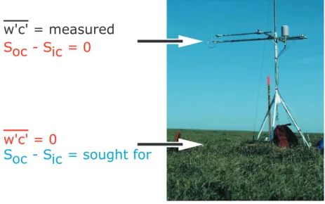
Figure 1 illustrates how the eddy covariance point measurement allows to quantify the net source and sink term in Eq. (1).

w'c' = measured

w'c' = 0 S - S = 0oc ic

S - S = sought foroc ic

Figure 1:Illustration of how the eddy covariance point measurement at one height relates to the net surface exchange (e.g. of CO₂, sensible heat, etc.). For simplification,∂c/∂t= 0is assumed.

Essentially we can derive the net ecosystem exchangeNEE =Soc −Sic, but not the two individual components. To be precise, the original equation also would allow for source and sink terms between measurement heightzand the surface atz= 0. For inert entities such as CO₂, non-condensing water vapor, sensible heat etc. it is however safe to postulate that no sources and sinks exist at heightsz > 0, which allows to relate the vertical eddy covariance flux term to the net surface exchange.

Another important physical matter of fact is that turbulence disappears if we approach the local surface. Every object in a turbulent medium is enveloped in a laminar layer, which is tiny, but more important which allows to postulatew⁰c⁰(z= 0) = 0.

As a result we can use the following equation to quantify net ecosystem exchange using the eddy covariance method at one single point in space:

NEE =w⁰c⁰(z) +z·∂c

∂t . (2)

In tall vegetation the storage termz∂c/∂tmay not be accurate enough and may require a more elaborate approach, typically a concentration profile measured at several heights across the canopy.

In any case however the storage term becomes negligibly small ifNEE is summed over days to months or years.

(4)

1.5 At which height should we measure?

Figure 2:Considerations about eddy covariance flux measurement height.

Figure 2 illustrates the concept of eddy covariance flux measurement height over tall vegetation. In this case, turbulence above the vegetation is a function of the distance above displacement heightd. Thus, the aerodynamic measurement heightz corresponds to the measurement heightZ above ground level, minus the displacement heightd: z = Z −d. As a rule of thumb,dis2/3of the canopy heighthcif the canopy is homogeneous.

Now if we measure too close to the canopy or even inside the canopy our flux measurements are subject to additional physical effect that we have not considered so far. Basically, the form drag effect describes turbulent flowaroundobstacles (tree truncs, individual plants) which re- sults in a non-random distribution of high and low turbulence conditions in space. Close to the surface we face the problem of the roughness sublayer where turbulence is not yet in full equilibrium with the vegetation surface roughness and may also lead to non-random patterns of turbulent conditions in space.

As another rule of thumb, the roughness length of a canopy isz₀≈0.1·h_c, and the roughness sublayer has the size ofz∗ ≈100·z0. Thus, we typically opt for a measurement heightz > z∗. In reality this is not always possible, especially over tall vegetation. Although this is considered a problem of the eddy covariance method by some scientists, one should keep in mind that the eddy covariance flux measurement is apoint information. Even inside the canopy and in the roughness sublayer we expecthighly accurateflux measurement, but the problem might be that this point measurement isnot automatically representative for the larger surface area that we are interested in. It would however be wrong to claim that the eddy covariance method fails under such conditions.

We should rather ask the question: do the turbulent fluxes tell us the whole story, or are there other mass transports (e.g. advection) that need to be quantified? And how can we relate our point measurement to the larger surface of interest?

(5)

2 Mathematical Details: Reynold’s Decomposition

Energy, mass and momentum are transported via turbulence elements which are called eddies (singular: eddy). Thus, for the quantification of a turbulent flux we postulate that we only have to keep track of tiny air parcels moving around with the 3-D wind vector and quantify the flux of energy, mass and momentum they carry with them (Fig. 3).

00 00

c c

w'=neg w'=neg

w'=pos w'=pos

c'=neg

c'=pos c'=pos

c'=neg

1

2 2

1

z z

Height above ground level Height above ground level

c c

Concentration Concentration

zEC zEC

F < 0_c F > 0_c

Figure 3:Idealized sketch showing the process of turbulent mixing in the vertical dimension (height above ground levelz). Left panel: turbulent net flux from the surface to the atmosphere (e.g. CO₂flux during the night when the atmosphere is stable, or sensible heat flux during the day when the atmosphere is unstable). Right panel: turbulent net flux from the atmosphere towards the surface (e.g. CO₂flux during the day when the atmosphere is unstable, or sensible heat flux during the night when the atmosphere is stable). After Stull (1988).

The nonlinear phenomenon called turbulence is approximated by a linearisation called Reynold’s decomposition:

a=a+a⁰ (3)

An overline denotes the mean value (temporal mean, in our case typically computed over a 30-minute interval), and a prime denotes the short-term deviation from that mean. Eddy covariance flux measurements require that the components are measured at high temporal res- olution, preferrably at 10 Hz or more.

This linearisation is by itself an approximation and is a very good approximation as long as

|a⁰| a. But recall that in the case of streamline co-ordinates we forcew= 0and thus in such a case|w⁰| wand thus from a mathematical viewpoint this Reynold’s decomposition is not necessarily a perfect way to linearise turbulent motions.

Knowing these limitations, we can profit from linear algebra after Reynold’s decomposition of our measured time series:

ab= (a·b) = (a+a⁰) b+b⁰

= a·b+a⁰b+ab⁰+a⁰b⁰

= a·b

+a⁰b+ab⁰+a⁰b⁰

= a·b+ 0 + 0 +a⁰b⁰

= a b+a⁰b⁰. (4)

(6)

3 Footprint or Source Area of Flux Measurements

Figure 4:Schematic of the source area of an eddy covariance flux measurement in 2-D cross-section. From Schmid and Oke (1990).

Figure 5:Characteristical dimensions of the source area:xm, distance to point of maximum contribution;a, prox- imal distance of surface influencing the measurement;e, distal distance of source area;d, maximum width of source area. These characteristic dimensions describe an isoline (thick line), which encompasses an area with a certain relative contribution to the overall measurement (e.g. 50% contribution). From Schmid (1994).

A simple model by Schmid (1994) allows to estimate the order of magnitude of the footprint size or source area of flux measurements. Each of the dimensionsD_Nin Figure 5 can be quantified by the following approximations.

For stable stratification (nighttime conditions) we use:

DN =α1· z

z₀ α2

·exp n

α3·z L

α4o

· σv

u∗

α5

, (5)

and for unstable stratification (daytime conditions) we use:

DN =α1· z

z0

α2

·

1−α3· z L

α4

· σv

u∗

α5

(6)

(7)

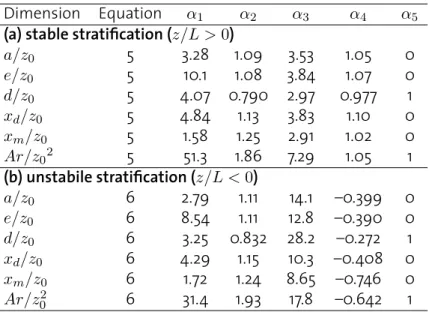
The parametersα1–α5and the dimension namesD_Ncan be taken from Table 1 (for mean values the footprint is much larger than for fluxes—see the original article by Schmid 1994).

Table 1: Parameters for the 50% source area contribution to eddy covarianceflux measurements. Dimensions (standardized by roughness lengthz0) are as in Figure 5, plusxdwhich is the distance of the sensors where the maximum width of the source area is found.Ar: total source area (standardized byz02).

Dimension Equation α₁ α₂ α₃ α₄ α₅ (a) stable stratification (z/L >0)

a/z₀ 5 3.28 1.09 3.53 1.05 0

e/z0 5 10.1 1.08 3.84 1.07 0

d/z₀ 5 4.07 0.790 2.97 0.977 1

x_d/z₀ 5 4.84 1.13 3.83 1.10 0 xm/z0 5 1.58 1.25 2.91 1.02 0 Ar/z₀² 5 51.3 1.86 7.29 1.05 1 (b) unstabile stratification (z/L <0)

a/z₀ 6 2.79 1.11 14.1 –0.399 0

e/z0 6 8.54 1.11 12.8 –0.390 0

d/z0 6 3.25 0.832 28.2 –0.272 1

x_d/z₀ 6 4.29 1.15 10.3 –0.408 0

xm/z0 6 1.72 1.24 8.65 –0.746 0

Ar/z₀² 6 31.4 1.93 17.8 –0.642 1

3.1 Online Footprint Computations

Kljun et al. (2004) have further developed this footprint area concept for flux measurements.

They computed a so called “master footprint” with a time-consuming computer model and then parameterized a simple approximation that allows to quickly estimate the footprint size using their web site http://footprint.kljun.net.

References

Kljun, N., P. Calanca, M. W. Rotach, and H. P. Schmid (2004) A simple parameterisation for flux footprint predictions.Boundary-Layer Meteorol.112, 503–523.

McMillen, R. T. (1988) An Eddy Correlation Technique With Extended Applicability to Non- Simple Terrain.Boundary-Layer Meteorol.43, 231–245.

Oke, T. R. (1987)Boundary Layer Climates(2nd ed.. ed.). London, New York: Methuen. 435 p.

Schmid, H. P. (1994) Source Areas For Scalars and Scalar Fluxes.Boundary-Layer Meteorol.67, 293–318.

Schmid, H. P. and T. R. Oke (1990) A Model to Estimate the Source Area Contributing to Turbu- lent Exchange in the Surface Layer Over Patchy Terrain.Quart. J. Royal Meteorol. Soc.116, 965–988.

Stull, R. B. (1988)An Introduction to Boundary Layer Meteorology. Dordrecht: Kluwer. 666 pp.

Zeman, O. and N. O. Jensen (1987) Modification of Turbulence Characteristics in Flow over Hills.Quart. J. Roy. Meteorol. Soc.113, 55–80.

(8)

4 Exercise 1: Calibrate H₂O Measurements

We carry out some test measurement with an eddy covariance system that has an open-path infra-red gas analyzer (IRGA) attached to it. This instrument was produced by?), measures CO₂ and H₂O concentration at 20 Hz, and has a curvilinear response.

We measure a signal in millivolts and need to calibrate that signal against a water vapor source to know how to translate millivolts into H₂O concentration values (we would need to do the same for CO₂but only focus on water vapor in this exercise).

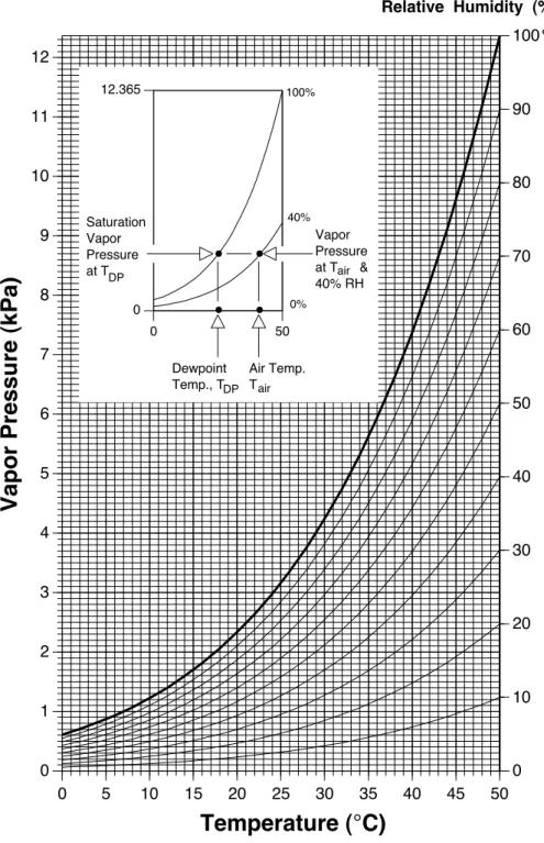
Calibrate the IRGA with a dew-point generator. To yield a curvilinear fit, we need at least three calibration points. The upper calibration point should be roughly the dewpoint of 80%

relative humidity at ambient temperature. Use the chart in Figure 6 to decide which dew-point temperature to take.

Use two lower (non-freezing!) dew points in addition to calibrate. Absolute humidityρ_v[kg/m³] is computed from vapor pressuree[kPa] as follows:

ρ_v = e T · p

p−e· 1

R_v ≈2.17· e

T , (7)

withT the air temperature [Kelvin],ppressure [kPa] in the optical path of the IRGA, andethe calibration vapor pressure in kPa.

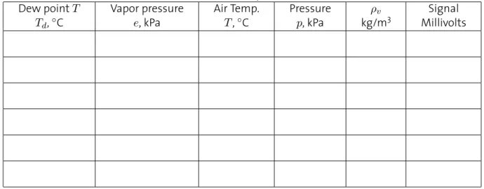
Table 2:Calibration protocol.

Dew pointT Vapor pressure Air Temp. Pressure ρ_v Signal

T_d,^◦C e, kPa T,^◦C p, kPa kg/m³ Millivolts

Then compute the best quadratic fit to your calibration points to convert millivolts to mmol/m³:

H₂O Concentrationρ_v[kg/m³] = + mV + (mV)²

(9)

Psychrometric Charts C-1

Appendix C. Psychrometric Charts

0 1 2 3 4 5 6 7 8 9 10 11 12

0 10 20 30 40 50 60 70 80 90 100

0 5 10 15 20 25 30 35 40 45 50

Temperature (°C)

0 12.365

0 50

% Relative Humidity (%)

Vapor Pressure (kPa)

• •

•

Air Temp.

T

Vapor Pressure at T &

40% RH Saturation

Vapor Pressure at T

Dewpoint Temp., T

100%

40%

0%

air

DP DP

air

•

Psychrometric Chart showing temperature, vapor pressure, and relative humidity (0 to 50 °C).

Figure 6:Psychrometric chart from the Licor 610 dew-point generator manual.

(10)

5 Exercise 2: Compute Fluxes

As an exercise to see what we actually do we take a 30-minute segment of raw data and process it ourselves in eitherRor another software package.

The raw data are saved in binary format, but we’ll convert them to an ASCII format that looks similar to this:

1.09 -1.32 0.51 338.32 493 1074 1.28 -1.30 0.64 338.32 493 1074 1.48 -1.09 0.36 338.24 495 1072

The first three columns areu,v, andzwind components in the co-ordinate system of the sonic anemometer; values are in m/s. The fourth column is speed of sound in m/s, and the remaining columns are millivolt signals from the IRGA. Depending on our configuration, the first signal is H₂O, the second is CO₂, and the third is IRGA temperature which we will not use.

1. Find out which of the signals actually is H₂O based on your calibration experiment 1 2. Convert the H₂O signal to absolute moistureρvin units of kg/m³

3. Determinew,c_H₂_O, andw⁰c⁰_H

2O

4. Determine the correlation coefficient ofw⁰andc⁰

5. Convert the moisture fluxw⁰ρv[kg/m²/s] into an evapotranspiration rateEof mm/hour 6. Convert the moisture fluxw⁰ρ⁰_v[kg/m²/s] into a latent heat flux in energy units [W/m²]

The latent heat of vaporization is (in units of J/kg):

Lv= [2.501−0.00237·(T −273.15)]·10⁶, (8) and the conversion to latent heat flux is then

LE =L_v·w⁰ρ⁰_v . (9)

We assume that the millivolt signal was converted to absolute moisture ρ_v using our calibration from exercise 1.

7. If possible compare the eddy covariance flux with the measurement of the lysimeter from the same hour (or half-hour interval, if available)

8. If possible compare the eddy covariance flux with the measurement from the evaporation pan for the same hour or better

(11)

6 Exercise 3: Analyze Diurnal Cycle

If weather permits we will try to measure a diurnal cycle. You’ll be given the computed fluxes to analyze the diurnal cycle. Gaps will be whenever we calibrated the IRGA or during rain showers.

If weather conditions are too bad then we’ll take a data set from another site for this exercise.

Merge the water vapor flux data with energy budget data. Plot the diurnal cycles of the energy balance

R_n=H+LE+G , (10)

whereR_nis net radiation,His sensible heat flux (from eddy covariance measurement),LEis latent heat flux (from eddy covariance measurement), andGis ground heat flux (if not measured, then determineGasG=R_n−H−LE).

Note on H: We measurew⁰T⁰with the eddy covariance system in units of K m/s. To yieldHin W/m₂we use the following equation:

H =ρ_a·c_p·w⁰T⁰ , (11) withρ_adensity of air [kg/m³], andc_p specific heat capacity of air at constant pressure (1005.5 J/kg/K).

Note on LE: In exercise 2 we converted our flux measurement to energy units; do the same for all half-hour fluxes in this exercise!