The Eddy Covariance Method

The Eddy Covariance Method

Exchange between earth and atmosphere is considered more and more relevant to climate studies. The earth surface appears to be an important source and sink, depending of the region and the moment considered, of water vapor, carbon dioxide, methane and other gases that are for instance used for vegetations respiration (Evapotranspiration accounts for the use of CO 2

and the emission of moisture). Assessing the exchange rates between soil surface and atmosphere and their variability is a key to a better understanding of the geochemical cycles and especially a way to quantify budgets, residence times and the vegetation’s effect as a part of the climate system.

Picture 1: Sonic anemometer and infra red gas analyzer.

The measurement of these budgets is done by the combined measurement of the 3 wind components and the gases concentration at high temporal frequency. By the using the Eddy Covariance method it is possible to derive the turbulent fluxes associated with those exchanges. The measurements are decomposed into a temporal mean term (average of the considered value over a certain time span) and a short term deviation to the mean:

!

u = u + u "

This so called Reynold’s decomposition is then used with concentration measurements to compute the vertical fluxes according to the Advection/Diffusion equation. This equation yields (no horizontal concentration and wind speed gradients are assumed, and coordinates are considered with respect to local stream lines):

!

" c

" t = # " w $ c $

" z + S _ource # S _ink

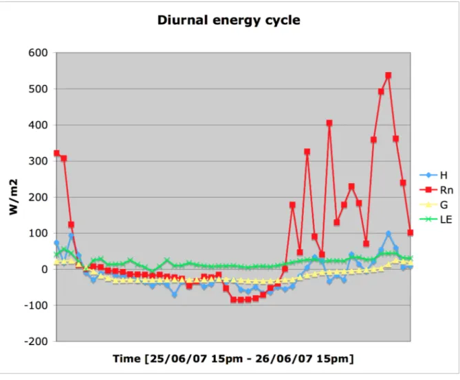
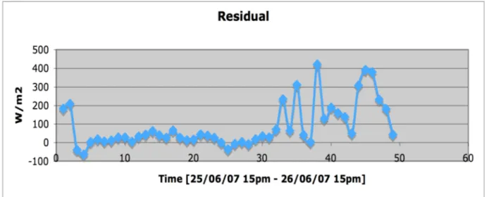
This method has been applied for CO 2 and H 2 O flux evaluation during the field course at the Rietzholdbach catchment area, on the 26 ^th of June 2007, and the purpose of this part is to show some results of this experiment.

1. Calibration:

The output data of the infrared gas analyzer yields mV values. A first step is to calibrate this output by using a known water vapor concentration generated with a dew-point generator and monitoring the instrument’s response. As this response is known to be non linear, at least 3 measurements are needed.

Dew point°C T inside °C Mean mV Abs humidity(g/m3)

Point 1 9 17 3498,642295 8,5673

Point 2 5 17,5 3130,059701 6,4994

Point 3 1 18,8 2834,860697 4,873

After fitting the data points we obtain:

H 2 O Concentration [kg/m ³ ] = -9.3968*10 ^-3 + 4,6*10 ^-6 * S +2*10 ^-10 * S ² where S is the signal in mV.

2. Fluxes

Reynold’s decomposition:

!

w = mean(w)

w = 0.38735184[m.s ^"1 ] C _H

₀ = mean(C _H

₀ )

C _H

₀ = 0.01103393[kg.m ^"3 ]

!

"

w = w # w

C _H

_O " = C _H

_O # C _H

_O

$

% &

' &

( " w ) C _H

_O " = mean( w " ) C _H

_O " )

"

w ) C _H

_O " = #5.53085 ) 10 ^#6 [kg.s ^#1 .m ^#2 ]

Correlation coefficient between w’ and c’:

!

Cor( w " , C _H

2

O " ) = #0.034242236

Evapotranspiration rate E:

!

E = w " # " _v $ 3600 = %0.019911[mm $ h ^%1 ]

Latent heat flux LE:

!

L _v = 2.45 " 10 ⁶ [J / kg]@293K

LE = L _v " # w $ # _v = %13.57[J " m ^%2 " s ^%1 ][W " m ^%2 ]

Comparison with Lysimeter data from the 26 ^th of June 2007, 13:30pm – 14:00pm local time:

During that time the Lysimeter hasn’t registered any runoff and no precipitation has fallen, meaning that all the weight loss must be due to Evapotranspiration during that time (ideally).

During that half hour, the weight off the Lysimeter dropped by 0.8kg (662.9-662.8 kg). The area covered by this measure is 3,14m ² and a difference of 3.14kg corresponds to 1mm water.

So this yields an evapotranspiration rate of:

E Lysimeter = 0,25 mm.h ^-1

The difference with the value derived from the Eddy Covariance method is 1 order of magnitude which is to high to be explained by experimental difference… I suspect an error in the use of the Eddy Covariance method calculation…

3. Diurnal cycle

The diurnal cycle (25/06/2007 15:00 – 26/06/2007 15:00) is computed on a half-an-hour basis from available radiation data and turbulent flux data.

R n = H + LE + G

• R n : net radiation [W/m ² ] – Computed from the “buel_YYYYMMDD.dat” files, and calibrated using the calibration file.

• H: sensible heat flux [W/m ² ] – Measured with the eddy covariance system in Km/s and converted to W/ m ² using H = ρ a *c p *ω’T’ (with ρ a =cst=1.2kg*m ^-3 ; c p =1005.5J*kg ^-1 *K ^-1 ).

• LE: latent heat flux [W/m ² ] – Computed using the H2O flux and the latent heat of vaporization of water (c.f. part. 2).

• G: ground heat flux [W/m ² ] – Computed from the “buel_YYYYMMDD.dat” files,

using the hourly measured flux. The missing half-an-hour values were obtained by

averaging the bracketing values.

The daily evolution of the energy balance (see next page) shows a strong daily cycle. During day, when the net radiation is the highest (due to higher incoming radiation), latent heat flux and sensible heat flux are high. During night, the net radiance is slightly negative (radiation from earth into space) and the other fluxes drop.

During day the high observed variability in the different fluxes and radiation can be due to the cloud cover, which was quite important that day, and cuts off net radiation and sensible heat.

But these measurements don’t verify the energy balance equation written before. This might be due to an error in the computation of the different fluxes and specially the latent heat flux as it is already reported above. The residual (Res=Rn-H-LE-G) is plotted in fig. 2.

Figure 1: Daily energy cycle measured from 15pm to 15pm the next day with half-an-

hour values.

Figure 2: Residual (Rn - H - LE - G )