What can we learn about QCD and collider physics from N = 4 super Yang-Mills?

What can we learn about QCD and collider physics from N = 4 super

Yang-Mills?

Johannes M. Henn

Max Planck Institute for Physics, Munich, Germany, 80805; email:

henn@mpp.mpg.de

Annu. Rev. Nucl. Part. Sci.: Submitted 2020. 71:1–30

https://doi.org/10.1146/annurev-nucl- 102819-100428

Copyright © 2020 by Annual Reviews.

All rights reserved

Keywords

scattering amplitudes, anomalous dimensions, Feynman integrals, N=4 super Yang-Mills theory, QCD

Abstract

Tremendous ongoing theory efforts are dedicated to developing new methods for QCD calculations. Qualitative rather than incremental advances are needed to fully exploit data still to be collected at the LHC. The maximally supersymmetric Yang-Mills theory (N = 4 sYM) shares with QCD the gluon sector, which contains the most complicated Feynman graphs, but at the same time has many special properties, and is believed to be solvable exactly. It is natural to ask what we can learn from advances in N = 4 sYM for addressing difficult problems in QCD.

With this in mind, we review here several remarkable developments and highlights of recent results in N = 4 sYM. This includes all-order results for certain scattering amplitudes, novel symmetries, surprising geometrical structures of loop integrands, novel tools for the calculation of Feynman integrals, and bootstrap methods. While several insights and tools have already been carried over to QCD and have contributed to state-of-the-art calculations for LHC physics, we argue that there is a host of further fascinating ideas waiting to be explored.

arXiv:2006.00361v2 [hep-th] 5 Jan 2021

Contents

1. INTRODUCTION . . . . 2

1.1. Motivation . . . . 2

1.2. Special properties of N = 4 super Yang-Mills . . . . 3

1.3. Scope of the review and related pedagogical reviews . . . . 4

1.4. Outline . . . . 4

2. THE CUSP ANOMALOUS DIMENSION . . . . 5

2.1. Maximal und uniform transcendentality principle . . . . 6

2.2. Exact result for planar cusp anomalous dimension . . . . 6

2.3. First non-planar corrections . . . . 7

3. AMPLITUDES IN N = 4 SUPER YANG-MILLS THEORY . . . . 8

3.1. Infrared divergences of amplitudes in the planar limit. . . . 8

3.2. Amplitudes at strong coupling . . . . 8

3.3. Duality between scattering amplitudes and Wilson loops . . . . 9

3.4. Dual (super)conformal symmetry . . . . 10

3.5. Discussion . . . . 10

4. LESSONS FROM LOOP INTEGRANDS . . . . 11

4.1. On-shell methods. . . . 11

4.2. Integrands with logarithmic singularities and uniform weight integrals . . . . 13

5. NOVEL METHODS FOR COMPUTING FEYNMAN INTEGRALS . . . . 14

5.1. Symbol method . . . . 15

5.2. Canonical differential equations method for computing Feynman integrals . . . . 16

6. INFRARED FINITE OBSERVABLES . . . . 18

6.1. Infrared finite loop integrals and amplitudes . . . . 18

6.2. Event shapes . . . . 19

7. BOOTSTRAPPING AMPLITUDES FROM THEIR ANALYTIC PROPERTIES . . . . 20

7.1. The bootstrap philosophy: return of the analytic S-matrix program . . . . 20

7.2. Extension of the bootstrap ansatz to multi-loop amplitudes. . . . 20

8. DISCUSSION AND CONCLUSION. . . . 22

8.1. How has N = 4 sYM knowledge fed into QCD calculations? . . . . 22

8.2. What more is possible? . . . . 22

1. INTRODUCTION 1.1. Motivation

Four-dimensional Yang-Mills theory, which is at the core of quantum chromodynamics (QCD), remains complicated, despite having been studied for more than half a century.

Only with great efforts can theoretical predictions be made that keep up with the accuracy of experimental data collected at the LHC. Compare this with developments in a close cousin of QCD, the maximally supersymmetric Yang-Mills theory, N = 4 super Yang-Mills (sYM). Many fantastic advances made over the last two decades make many researchers think that, at least in the planar limit, the theory may be solved exactly! The two theo- ries share the Yang-Mills sector, so that tree-level gluon amplitudes are identical in both theories. Although the gluon amplitudes differ at loop level due to the matter content, the gluon diagrams, which are the most complicated ones, are the same.

What can we learn from progress in N = 4 sYM for QCD calculations? In this review

we wish to share the excitement about surprising and remarkable results, and to convey

the conceptual and technological advances that led to them. Moreover, we wish to point out where this research has already led to a transfer of knowledge to QCD. We also hope that by outlining recent developments, this review will help to promote positive exchange among the research communities.

We intend this review to be accessible (and hopefully enjoyable!) to non-expert read- ers from various fields of science, including researchers and students from fields such as experimental physics or phenomenology, or QCD practitioners, who are curious to know more about this subject. Some readers may wish to get an overview of this research area to see if there are interconnections to other work. Others may have heard buzzwords such as ‘transcendentality’, ‘symbol’, ‘amplituhedron’, ‘bootstrap’, and so on. In the following pages, we aim to explain those terms in a non-technical way.

Some readers might ask themselves whether studies in N = 4 sYM, however rewarding they may be in their own right, are not somewhat esoteric, in the sense that they seem far removed from the gritty calculations of ‘real’ QCD. In some cases it can be beneficial to view QCD as a perturbation around N = 4 sYM, but this has limited scope. Our viewpoint is rather that we can learn about new concepts in quantum field theory that would be hard to discover in a more complicated Yang-Mills theory. A particularly interesting topic is understanding physically motivated singular limits, such as the important high-energy or collinear limits, where one often finds universal behavior. New insights into N = 4 sYM have already led to novel tools for QCD, and are being used for cutting edge calculations relevant to LHC physics. Beyond this, there is a host of further ideas and concepts available in the

‘ N = 4 sYM world’, that have been considered only very recently, and whose potential for generalization to other theories is yet to be explored. M. Shifman (1) describes this philosophy very clearly as follows: “Although the ultimate goal [...] is calculating QCD amplitudes, the concept design of various ideas and methods is carried out in supersymmetric theories, which provide an excellent testing ground. Looking at super-Yang-Mills offers a lot of insight into how one can deal with the problems in QCD.”

With this in mind here are a few concrete questions we think are important:

• Can we develop methods to systematically compute Feynman integrals in QCD?

• Can we compute physical quantities without explicitly evaluating Feynman diagrams?

• How can our calculations benefit from knowledge of physical properties of the under- lying QFT, such as unitarity, space-time symmetries, and conformal invariance?

• Can we compute finite physical quantities in a way that avoids infrared singularities?

• Which properties of QCD scattering amplitudes are governed by Wilson loops?

1.2. Special properties of N = 4 super Yang-Mills

The maximally supersymmetric Yang-Mills theory is often considered an idealized toy model for a possibly solvable four-dimensional Yang-Mills theory. Its Lagrangian can be written most compactly in ten-dimensional notation,

L = tr

− 1

2 F

M N

F

^{M N}

+ iΨΓ

^N

DΨ

, 1.

where D is a covariant derivative, and F

^{M N}

is the ten-dimensional field strength. The

four-dimensional Lagrangian is then obtained by dimensional reduction, i.e. assuming that

the fields only depend on the first four space-time dimensions. Moreover, one writes the

ten-dimensional gauge field as A

^M

= (A

^µ

, φ

ⁱ

) , where A

^µ

is the usual four-dimensional gauge

field, and φ are six real scalars. In this way one obtains a four-dimensional Lagrangian that contains gluons coupled canonically to the scalars and to four complex fermions. Further- more, there are Yukawa and quartic scalar interaction vertices, in such a way as to preserve N = 4 supersymmetry, see e.g. (2). All fields are in the adjoint representation of SU(N ) . It is important to note that many of the methods discussed in this review do not rely on the explicit Lagrangian.

The theory has many special properties in addition to being supersymmetric. The combination of scale and Poincaré invariance of the Lagrangian lead to invariance under a larger continuous group, the conformal group, which includes translations, rotations and boosts, scale transformations, and coordinate inversions. In four dimensions, in which the Lorentz group is isomorphic to SO(3,1), the conformal group is isomorphic to SO(4,2). This leads to powerful constraints. It is striking that this symmetry is not broken by quantum corrections, as the theory has a vanishing beta function to all orders in perturbation theory (3, 4).

Conformal group:

Extension of the Poincaré group to all transformations that preserve angles (in Euclidean space).

Moreover, the AdS/CFT correspondence conjectures a duality between d-dimensional conformal field theory and string theory in (d + 1)-dimensional anti de-Sitter space (5, 6, 7).

The duality comes with a ‘dictionary’ that relates observables in the different theories. One of the best studied cases of the duality is N = 4 sYM on the one hand, and string theory on AdS

5

space on the other hand. The nature of this duality, which relates field theory at strong coupling to string theory at weak coupling, implies that the perturbative series must have special properties. Remarkably simple structures have indeed been observed, e.g. for anomalous dimensions and especially in recent years, for scattering amplitudes. Indeed, it appears that N = 4 sYM ‘wants’ to teach us about nice mathematical structures, and all we need to do is to investigate interesting quantities in the theory and study their properties.

1.3. Scope of the review and related pedagogical reviews

The focus of this review is on developments related to scattering amplitudes. The reason for this is twofold. On the one hand, scattering amplitudes are obviously of interest for collider physics, which is timely in view of the third run of the LHC. On the other hand, this has been and continues to be a particularly active area in N = 4 sYM, and we think that there is considerable potential in applying insights from that theory to QCD calculations.

Scattering amplitudes: Key ingredients of cross sections, analogous to probability amplitudes in quantum mechanics.

Given the wealth of results accumulated over many years, it is very difficult to make a selection. It would have been possible to write a review four times this length, covering important topics in more detail, and giving full justice to the many developments discussed for example at the yearly Amplitudes conferences. A guiding principle was primarily to present developments that have potential for application in more general settings, or are surprising, such as all-orders results for certain quantities in an interacting four-dimensional gauge theory.

References to the original literature are given as much as possible to help readers learn more. We also point out a number of related resources, after the list of references. These include several review articles on scattering amplitudes, as well as on closely related research areas, such as integrability in planar N = 4 sYM, and conformal methods.

1.4. Outline

Sections 2 and 3 focus on selected highlights of exact results, with the intention of giving the

reader a taste of what may be possible in a four-dimensional gauge theory. We then focus on

(a) (b) (c)

Figure 4. Examples of Feynman diagrams contributing to the vertex functionV

(φ) at one loop (a) and two loops, (b) and (c). The diagram (b) does not contribute to the right-hand of (2.17).

V (0) leading to [7]

log W = log V (φ) − logV (0) = logZ + O(ϵ

⁰

). (2.16) This relation allows us to compute log Z from the subset of Feynman diagrams correspond- ing to vertex corrections V (φ), i.e. with non-trivial angular dependence.

2.4 Nonabelian exponentiation

The calculation of the cusp anomalous dimension can be significantly simplified by making use of the nonabelian exponentiation property of the Wilson loop [22, 23, 66]. It allows us to express a logarithm of the Wilson loop, log W , in terms of a special class of ‘maximally nonabelian’ diagrams, the so-called webs.

In the special case of gauge theories in which all fields are defined in the adjoint representation of SU(N), this leads to the following general expression

log W = C

R

!

3

n=1

" α

s

π

#

n

C

ⁿ_A⁻¹

[V

n

(φ) − V

n

(0)] + O(α

⁴s

) , (2.17)

where C

A

= N is the quadratic Casimir operator of SU(N ) in the adjoint representation, f

^abc

f

^and

= C

A

δ

^cd

, and V

n

(φ) stands for the sum of certain Feynman integrals defining n − loop corrections to the (one-particle irreducible) vertex function (see figure 4). Notice that the expression on the right-hand side of (2.17) only depends on the quadratic Casimirs.

In addition, it is proportional to C

R

that depends on the representation in which the Wilson loop (2.1) is defined, the so-called Casimir scaling. It is expected that both properties are violated at four loops since the color factors start to depend on higher Casimirs of SU(N ).

The power of the nonabelian exponentiation (2.17) is that it allows us to discard the diagrams whose color factor does not contain terms of the maximally nonabelian form.

Moreover, we can use (2.17) to express their contribution in terms of Feynman integrals V

n

that appear on the right-hand side of (2.17). To illustrate this point consider the Feynman diagrams shown in figure 4. The one-loop diagram shown in figure 4(a) has the color factor C

R

and the corresponding Feynman integral defines V

1

(φ). The two-loop diagrams shown in figures 4(b) and (c) have the color factors C

_R²

and C

R

(C

R

− C

A

/2), respectively.

– 9 –

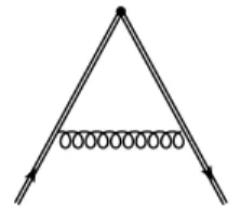
Figure 1: One-loop Feynman diagram contributing to the vacuum expectation value of a Wilson loop formed by two segments. The leading short-distance divergence defines the cusp anomalous dimension.

perturbation theory, where one hopes to see the closest similarities with QCD. Many explicit results for amplitudes are in some sense the tip of the iceberg, and in part are made possible and supported by a large body of work on loop integrands, which is the topic of section 4. In section 5 we then discuss new techniques for Feynman integrals and for the special functions arising in them. In section 6 we consider prospects for computing infrared finite Feynman integrals and observables. The ‘bootstrap’ method for higher loop amplitudes in section 7 brings together many of these ideas. The conclusion follows in section 8. At different places in the review there are wide blue boxes highlighting fascinating related subjects that are not discussed in the main text but may be of interest for further reading.

2. THE CUSP ANOMALOUS DIMENSION

In quantum field theory, anomalous dimensions are important quantities. In QCD, the scal- ing evolution of parton distributions is governed by the anomalous dimension of composite operators. In a conformally invariant field theory, scaling dimensions are fundamental be- cause they govern the short-distance properties of correlation functions via the operator product expansion (8).

Cusp anomalous dimension:

Determines the leading soft and collinear divergences of scattering amplitudes.

The cusp anomalous dimension is of particular interest. It is defined from the vacuum expectation value of certain Wilson loops,

hW

C

i = htr P exp

ig I

C

A

µ

dx

^µ

i , 2.

where the integral is along a closed contour C , and P stands for path ordering of the SU(N) -valued field A

µ

along the contour. When the contour C is not smooth, but contains a cusp as in Figure 1, then there are short-distance divergences, which are controlled by the cusp anomalous dimension (9). One can equivalently interpret the anomalous dimension as describing divergences due to soft gluon exchanges between two particles whose classical trajectories are given by the two segments of the contour, or due to virtual gluons emitted and absorbed by a particle that is hard-scattered at the point of the cusp.

We discuss here the case where the cusp is formed by two null, or light-like, segments (10), and we denote the associated anomalous dimension by Γ

cusp

. It depends on the Yang-Mills coupling g

Y M

, and on the rank N of the gauge group SU(N ) .

Its importance comes from the fact that it appears in many quantities. For example, it

controls the large spin behavior of twist two operators (10), and it governs soft and collinear

divergences of form factors and scattering amplitudes (11, 12). It also plays a prominent role

in the high-energy (Regge) limit (13), and more generally often appears in special singular

limits.

In the following sections we will frequently discuss N = 4 sYM in the limit N → ∞, while keeping the ‘t Hooft coupling g

²

= g

²YM

N/(16π

²

) fixed (14). In this limit, planar diagrams dominate, and diagrams of higher genus G are suppressed by factors of N

^−2G

. Unless otherwise stated, quantities in this and in the next section are assumed to be in this limit. We can then write

Γ

cusp

(g) = X

L≥1

g

^2L

Γ

^(L)_cusp

, 3.

for the perturbative expansion of the cusp anomalous dimension, and analogously for other quantities.

Planar limit:

Combined limit of the rank of the gauge group and of the coupling, so that planar Feynman diagrams dominate.

2.1. Maximal und uniform transcendentality principle

Let us start by looking at perturbative results for the cusp anomalous dimension. Its three-loop value in N = 4 sYM is (15)

Γ

cusp

=

g

²_YM

N 4π

²

− π

²

12

g

_YM²

N 4π

²

²

+ 11π

⁴

720

g

_YM²

N 4π

²

³

+ O(g

YM⁸

) . 4.

Looking at Equation 4 one notices an intriguing pattern. All transcendental constants appearing in this formula are instances of zeta values ζ

n

= P

k≥1

1/k

ⁿ

, for example, ζ

2

= π

²

/6 . Moreover, if one assigns transcendental weight, or ‘transcendentality’ n to ζ

n

, then the coefficients at L loops have weight 2L − 2 .

Transcendental weight: partly heuristic but useful property of transcendental constants and iterated integrals (see section 5).

It is instructive to compare Equation 4 to its corresponding result in QCD without quarks,

Γ

^QCD_cusp

= C

R

g

_YM²

4π

²

+ C

R

C

A

g

_YM²

4π

²

2

− π

²

12 + 67

36

+

+C

R

C

_A²

g

YM²

4π

²

3

11π

⁴

720 + 11ζ

3

24 − 67π

²

216 + 245

96

+ O(g

⁸_YM

) , 5.

Here C

R

and C

A

= N are quadratic Casimir operators of SU(N ) . R refers to the repre- sentation of the fields under consideration. Setting R = A for the adjoint representation, we see a remarkable feature of Eqs. 4 and 5: the leading transcendental weight terms agree between N = 4 sYM and QCD (16, 17)!

This agreement of the ‘most complicated terms’ was predicted based on an argument that the leading weight contribution to this quantity comes entirely from gluons (17). On the other hand, more general quantities, such as scattering amplitudes, may have maximal weight terms differing from those in N = 4 sYM.

Nevertheless, in retrospect the qualitative pattern that quantities in N = 4 sYM have maximal weight turned out to be very important. The notion of weight generalizes to functions, as we will see in section 4.2 and 5. All evidence to date supports that L-loop scattering amplitudes in N = 4 sYM have uniform and maximal weight 2L .

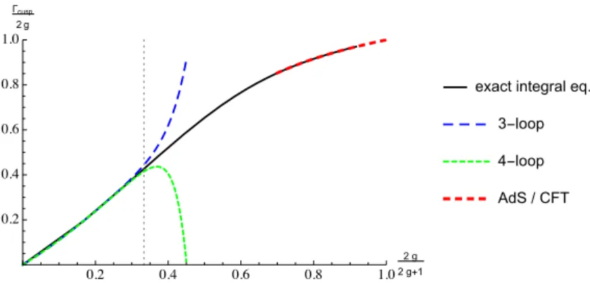
2.2. Exact result for planar cusp anomalous dimension

The cusp anomalous dimension is a prominent example of the application of integrability-

based approaches in N = 4 sYM. As far as we are aware, there is no unambiguous or

commonly agreed-upon definition of integrability in quantum field theory. Usually it refers

��� ��� ��� ��� ���

2 g 2 g+1

���

���

���

���

���

Γcusp 2 g

exact integral eq.

3-loop 4-loop AdS / CFT

Figure 2: Planar cusp anomalous dimension plotted on the whole range from weak to strong coupling, with g

²

= g

Y M²

N/(16π

²

). The numerical solution of an exact integral equation (22) (solid line) agrees well with the three- and four-loop perturbative approximations, within the radius of convergence g = 1/4 (vertical dashed line). It also agrees with the strong coupling expansion obtained from string theory. Figure adapted from (23).

to a situation where (hidden) symmetries allow a problem to be solved exactly, to all orders.

Here ‘exactly’ could mean that the problem is recast in terms of a set of equations that in principle determine the answer (that may still involve complicated functions). One reason for thinking that N = 4 sYM theory may be integrable is the AdS/CFT correspondence, as signs of integrability are found in string theory (18, 19).

Following earlier work in QCD, reviewed in (20), it was realized that anomalous dimen- sions of composite operators in the theory are equivalent to energies in certain integrable spin chain models (21). For example, at one loop the Heisenberg spin chain known from condensed matter physics makes an appearance. While the precise spin chain Hamiltonian was worked out explicitly only to low loop orders, it was the starting point for exploring integrability in planar N = 4 sYM. Assuming a Bethe ansatz inspired by integrability, the cusp anomalous dimension is described by an integral equation valid to all orders in the coupling (22). A truly impressive discovery! The predictions of the latter agree with four-loop quantum field theory results (24), as well as (25, 26) with string theory results at strong coupling coupling (27, 28), see Figure 2. Related to this there are first promising numerical results from a novel AdS/CFT lattice approach (29).

2.3. First non-planar corrections

Integrability results for the cusp anomalous dimension are currently limited to the planar limit. Non-planar corrections to the cusp anomalous dimension appear for the first time at four loops and have recently been obtained analytically (30, 31),

Γ

cusp

= ( Eq. 4) − 73π

⁶

20160 + ζ

₃²

8 + 1

N

²

31π

⁶

5040 + 9ζ

₃²

4

g

_YM²

N 4π

²

4

+ O(g

¹⁰_YM

) . 6.

It is interesting to mention that taking into account known simpler contributions from

fermions and scalars, the N = 4 sYM result provided the last missing ingredient to the full

color dependence of the four-loop QCD cusp anomalous dimensions (30), which was later

reproduced by a direct QCD computation (32).

3. AMPLITUDES IN N = 4 SUPER YANG-MILLS THEORY 3.1. Infrared divergences of amplitudes in the planar limit

The study of the structure of infrared divergences in gauge theories has a long history. A key concept is the idea of factorization. Specifically, effects coming from soft and collinear emissions decouple, and hence can be written in a factorized form. The collinear terms are universal and independent of the scattering process. The soft terms can be represented by emission from Wilson lines tracing the initial and final particle directions.

As an example, consider some scattering process involving a virtual gluon exchanged between two on-shell legs. In the region of integration where the momentum k of the gluon becomes soft, i.e. k → 0 , the scattering amplitude factorizes as

(a)(b)(c)

Figure4.ExamplesofFeynmandiagramscontributingtothevertexfunctionV(φ)atoneloop(a)andtwoloops,(b)and(c).Thediagram(b)doesnotcontributetotheright-handof(2.17).

V(0)leadingto[7]

logW=logV(φ)−logV(0)=logZ+O(ϵ0).(2.16)

ThisrelationallowsustocomputelogZfromthesubsetofFeynmandiagramscorrespond-ingtovertexcorrectionsV(φ),i.e.withnon-trivialangulardependence.

2.4Nonabelianexponentiation

ThecalculationofthecuspanomalousdimensioncanbesignificantlysimplifiedbymakinguseofthenonabelianexponentiationpropertyoftheWilsonloop[22,23,66].ItallowsustoexpressalogarithmoftheWilsonloop,logW,intermsofaspecialclassof‘maximallynonabelian’diagrams,theso-calledwebs.

InthespecialcaseofgaugetheoriesinwhichallfieldsaredefinedintheadjointrepresentationofSU(N),thisleadstothefollowinggeneralexpression

logW=CR 3!

n=1 "αsπ #nCn−1A[Vn(φ)−Vn(0)]+O(α4s),(2.17) whereCA=NisthequadraticCasimiroperatorofSU(N)intheadjointrepresentation, fabcfand=CAδcd,andVn(φ)standsforthesumofcertainFeynmanintegralsdefiningn−loopcorrectionstothe(one-particleirreducible)vertexfunction(seefigure4).Noticethattheexpressionontheright-handsideof(2.17)onlydependsonthequadraticCasimirs.

Inaddition,itisproportionaltoCRthatdependsontherepresentationinwhichtheWilsonloop(2.1)isdefined,theso-calledCasimirscaling.ItisexpectedthatbothpropertiesareviolatedatfourloopssincethecolorfactorsstarttodependonhigherCasimirsofSU(N).Thepowerofthenonabelianexponentiation(2.17)isthatitallowsustodiscardthe

diagramswhosecolorfactordoesnotcontaintermsofthemaximallynonabelianform.Moreover,wecanuse(2.17)toexpresstheircontributionintermsofFeynmanintegralsVnthatappearontheright-handsideof(2.17).ToillustratethispointconsidertheFeynmandiagramsshowninfigure4.Theone-loopdiagramshowninfigure4(a)hasthecolor

factorCRandthecorrespondingFeynmanintegraldefinesV1(φ).Thetwo-loopdiagramsshowninfigures4(b)and(c)havethecolorfactorsC2RandCR(CR−CA/2),respectively.

–9–

k ^(a)(b)(c)

Figure4.ExamplesofFeynmandiagramscontributingtothevertexfunctionV(φ)atoneloop(a)andtwoloops,(b)and(c).Thediagram(b)doesnotcontributetotheright-handof(2.17).

V(0)leadingto[7]

logW=logV(φ)−logV(0)=logZ+O(ϵ0).(2.16)

ThisrelationallowsustocomputelogZfromthesubsetofFeynmandiagramscorrespond-ingtovertexcorrectionsV(φ),i.e.withnon-trivialangulardependence.

2.4Nonabelianexponentiation

ThecalculationofthecuspanomalousdimensioncanbesignificantlysimplifiedbymakinguseofthenonabelianexponentiationpropertyoftheWilsonloop[22,23,66].ItallowsustoexpressalogarithmoftheWilsonloop,logW,intermsofaspecialclassof‘maximally

nonabelian’diagrams,theso-calledwebs.InthespecialcaseofgaugetheoriesinwhichallfieldsaredefinedintheadjointrepresentationofSU(N),thisleadstothefollowinggeneralexpression

logW=CR 3!

n=1 "αsπ #nCn−1A[Vn(φ)−Vn(0)]+O(α4s),(2.17) whereCA=NisthequadraticCasimiroperatorofSU(N)intheadjointrepresentation,fabcfand=CAδcd,andVn(φ)standsforthesumofcertainFeynmanintegralsdefiningn−loopcorrectionstothe(one-particleirreducible)vertexfunction(seefigure4).Noticethattheexpressionontheright-handsideof(2.17)onlydependsonthequadraticCasimirs.

Inaddition,itisproportionaltoCRthatdependsontherepresentationinwhichtheWilsonloop(2.1)isdefined,theso-calledCasimirscaling.ItisexpectedthatbothpropertiesareviolatedatfourloopssincethecolorfactorsstarttodependonhigherCasimirsofSU(N).Thepowerofthenonabelianexponentiation(2.17)isthatitallowsustodiscardthe

diagramswhosecolorfactordoesnotcontaintermsofthemaximallynonabelianform.Moreover,wecanuse(2.17)toexpresstheircontributionintermsofFeynmanintegralsVnthatappearontheright-handsideof(2.17).ToillustratethispointconsidertheFeynman

diagramsshowninfigure4.Theone-loopdiagramshowninfigure4(a)hasthecolorfactorCRandthecorrespondingFeynmanintegraldefinesV1(φ).Thetwo-loopdiagramsshowninfigures4(b)and(c)havethecolorfactorsC2RandCR(CR−CA/2),respectively.

–9–

k→ 0 k

∼

^×

…

… ^{. 7.}

Here the blob denotes some hard scattering process (i.e. no further loop momenta are soft or collinear). The physical meaning of Equation 7 is that soft gluons do not probe the hard scattering process. The leading divergence of the vertex diagram on the right hand side of the equation is precisely the (one-loop value of) the cusp anomalous dimension.

Being an ultraviolet finite theory, N = 4 sYM is a particularly good testing ground for understanding infrared divergences. One encounters them in their purest form, disentangled form ultraviolet divergences. In particular, in the planar limit, the divergences of an n-gluon amplitude A

n

, regulated dimensionally with D = 4 − 2, take the form

A

n

= A

⁽⁰⁾n

exp ( X

L≥1

g

^2L

X

n

i=1

− Γ

^(L)cusp

4(L)

²

− G

₀^(L)

4L

µ

²

s

i i+1

^L

+ F

n

(g; s

ij

) + O() )

. 8.

Here A

⁽⁰⁾n

is the tree-level amplitude, G

0

is the collinear anomalous dimension (33), and F

n

is the finite part. µ

²

is the dimensional regularization scale, and s

ij

= 2p

i

· p

j

, where p

i

are the on-shell gluon momenta, and s

n n+1

= s

1n

. We see that Equation 8 has a factorized structure (34, 35). Its particularly simple form is due to the planar limit, where soft/collinear exchanges can occur only between two particles at a given time. The latter lead to infrared divergences, which are represented by single and double poles in in Eq. 8.

3.2. Amplitudes at strong coupling

In the previous section we saw that the planar cusp anomalous dimension is known. Sur- prisingly, the same is true for certain scattering amplitudes. In (37, 15), based on three-loop calculations, an all-orders guess was put forward for the finite part of the planar four-gluon amplitude in N = 4 sYM,

F

4

(g; t/s) = 1

4 Γ

cusp

(g) log

²

(t/s) + C(g) , 9.

with s = s

12

and t = s

23

. This means that in addition to the exponentiation of the

infrared divergences, the finite part also exponentiates in a very simple way. Apart from

the scheme-dependent constant C(g) , Equation 9 predicts the full kinematic dependence

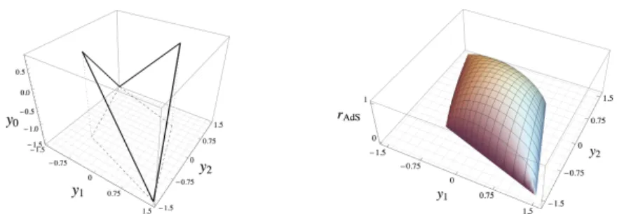
Figure 3: Left: Null polygon formed by the four gluon momenta, for s/t = 4 . Right:

Minimal surface area solution of (36), projected onto the (y

1

, y

2

) plane. The surface ends at r _AdS = 0 on the null polygon. It extends into the radial direction, similar to a soap bubble. Both plots use Poincaré coordinates (y

^µ

, r _AdS ) .

of the amplitude, at any order of the coupling. In particular, Equation 9 predicts the amplitudes at strong coupling.

The AdS/CFT duality relates observables in the gauge theory and in string theory.

Until 2007, studies focused on correlation functions, anomalous dimensions and Wilson loops in the theory. In a breakthrough paper (36), it was shown that the computation of planar gluon scattering amplitudes at strong coupling is equivalent to a minimal surface area calculation in AdS

5

space, with the surface ending on a polygon formed by the gluon momenta. See Fig. 3 for the four-particle case. The polygon is closed due to momentum conservation. Amazingly, the regularized minimal surface area (36) agrees perfectly with Equations 8 and 9.

AdS

5

:

Anti-de-Sitter space, whose boundary at r

AdS

= 0

corresponds to four-dimensional Minkowski space-time.

3.3. Duality between scattering amplitudes and Wilson loops

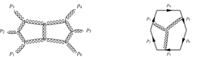
According to the AdS/CFT dictionary, a minimal surface area calculation corresponds to the vacuum expectation value of a Wilson loop. Therefore the work of (36) suggested a duality between scattering amplitudes and Wilson loops at strong coupling. Subsequently, the duality was found to hold also at weak coupling, first for the maximally-helicity-violating (MHV) (38, 39), and later for general helicity configurations (40). The most non-trivial test is probably the agreement of the two-loop six-gluon MHV amplitude and the corresponding hexagonal Wilson loop (41, 42). Further evidence for the duality holding at all orders in the coupling was provided by a string theory argument in (43). See (44) for a review.

MHV: The simplest non-trivial helicity configuration of gluon scattering amplitudes in supersymmetric Yang-Mills theory.

It is remarkable that scattering amplitudes can be computed from Wilson loops. The latter usually appear in special limits or in effective theories, such as heavy-quark effective theory (45) and soft-collinear effective theory (46). What is truly remarkable here is that they describe not only the divergences, but also the finite part.

The Wilson loop picture offers several conceptual advantages. Firstly, while the scat-

tering amplitudes have infrared divergences, the Wilson loops have ultraviolet (cusp) diver-

gences. The structure of the latter is much easier to understand thanks to exponentiation

properties of the eikonal lines (47). Secondly, the collinear limit of amplitudes corresponds

to flattening one of the cusps in the Wilson loop picture. It turns out that not only the

universal leading term, but also the near-collinear limit can be described using powerful

operator product expansion techniques (48, 49, 50, 51). Thirdly, at the practical level, Wil-

son loops are typically easier to evaluate than scattering amplitudes, so that the duality

+ … p

₁

p

₂

p

₃

p

₄

p

₅

p

₆

p

₁

p

₂

p

₃

p

₄

p

₅

p

₆

𝒜(p

1

, …, p

₆

) =

⟨W

₆

⟩ = + …

+ … p₁

p₂

p₃ p₄

p₅ p₆

p₁ p₂ p₃

p₄ p₅

p₆ 𝒜(p1, …,p₆) =

⟨W6⟩ = + …

Figure 4: Sample Feynman diagrams contributing to the two-loop six-gluon amplitude (left), and to the two-loop hexagonal Wilson loop (right).

brings about technical simplification. This can be seen by the fact that one can evaluate numerically certain n -particle Wilson loops at two loops (52) at any value of n . Much progress has occurred for the corresponding dual amplitudes, but currently their numerical evaluation in generic kinematics is limited to seven particles (53, 54, 55, 56).

3.4. Dual (super)conformal symmetry

Early hints at a hidden symmetry of scattering amplitudes were seen in special properties of the loop integrand (57) of the four-gluon amplitude. In the Wilson loop picture, the hidden symmetry is obvious: it is the coordinate-space conformal symmetry that transforms covariantly the polygon with light-like edges on which the Wilson loop is defined. For the amplitudes, it becomes a dual conformal symmetry (acting in momentum space), in addition to their coordinate space conformal symmetry.

The symmetry can be used to make quantitative predictions. The cusp divergences of the Wilson loop break the symmetry slightly, but in a way controlled by all-order Ward identities (58). The latter are very powerful: they fix the kinematic dependence for four and five gluons, in agreement with Equation 9. Moreover, the general n-gluon formula with n > 5 is essentially given by the exponentiation of the one-loop result, with coefficient Γ

cusp

, plus a function of 3n − 15 dual conformal invariants. This is to be compared with 3n − 11 variables without the symmetry. For six gluons, this means three instead of seven variables!

The new dual conformal symmetry is part of a dual superconformal algebra (59, 43).

When combined with the original superconformal symmetry of the Lagrangian, one obtains a Yangian algebra (60), which is a hallmark of integrability. Interestingly, some of the dual superconformal symmetry generators are also anomalous and lead to powerful relations between amplitudes involving different number of external legs and loop orders (61).

Yangian:

Infinite-dimensional Hopf algebra that often appears in two-dimensional QFTs and in spin chain models.

While most studies in N = 4 sYM focus on massless scattering amplitudes, there is a natural way of introducing masses within the AdS/CFT correspondence. In this way, one can define infrared finite amplitudes that have an exact dual conformal symmetry (62).

3.5. Discussion

Some readers might think that a mysterious hidden symmetry is quite far removed from reality even more so in a conformal theory. However, upon closer inspection dual conformal symmetry is much more familiar than it may seem. The new generator it provides is equivalent (63) to the well-known Runge-Lenz vector. It is responsible for the regularity of planetary orbits in the Kepler problem in classical mechanics, and it explains the simplicity spectrum of the hydrogen atom in quantum mechanics (64).

Runge-Lenz vector:

Additional constant

of motion describing

the shape and

orientation of an

elliptical planetary

orbit.

Does the scattering amplitudes / Wilson loops duality and dual conformal symmetry extend to the non-planar sector (65, 66)? Genuine non-planar corrections to amplitudes start at two loops, and although difficult to obtain, some results are available for further investigations (67, 68, 69).

What can we learn from the fascinating results and dualities in N = 4 sYM for QCD?

First, symmetries play an important role in the N = 4 sYM story. It would be interesting to disentangle the role of conformal symmetry from that of the extended supersymmetries.

How powerful are the consequences of conformal symmetry alone, for example, for QCD at a conformal fixed point? Second, QCD and N = 4 sYM are more similar in singular limits.

Does this indicate that these are universal properties of Yang-Mills gauge theories? Third, having a Yang-Mills theory where results are known to high orders in perturbation theory, or even exactly, gives us a unique perspective on what may be possible in any gauge theory.

Indeed, many people would argue that the surprising simplicity of final results obtained in N = 4 sYM suggests that there are better ways of thinking about quantum field theory.

These could well lead to new practical tools for QCD calculations, and perhaps even to new perspectives on the foundations of quantum field theory.

THE MULTI-REGGE LIMIT OF QCD AND N = 4 SUPER YANG-MILLS

QCD and supersymmetric Yang-Mills theories share the gluon sector, and in a qualitative sense this contains the most complicated diagrams. In certain physical regimes, gluons also give quantitatively the main contributions. This means that one can hope to find common properties in those limits. This is the case for the multi-Regge limit, which plays an important role for multi-particle amplitudes in N = 4 sYM (70), see section 7. In QCD integrability was first seen in this limit, including a two-dimensional version of dual conformal symmetry (71, 72). Moreover, while this is not the case for general kinematics, in this limit amplitudes in QCD are related to Wilson loops (13).

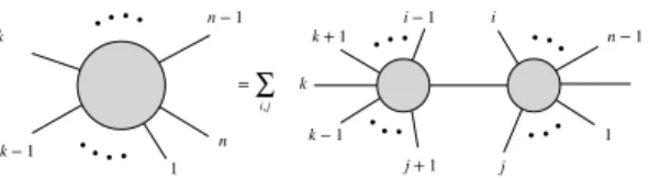
4. LESSONS FROM LOOP INTEGRANDS 4.1. On-shell methods

An important conceptual principle in scattering amplitudes is to work as much as possible with gauge-invariant objects. The reason is that individual Feynman diagrams are not gauge invariant, but scattering amplitudes – sums of Feynman diagrams evaluated on-shell – are. For tree and one-loop diagrams, the off-shell expressions are often very complex, but they dramatically simplify when they are evaluated on-shell.

It turns out that it is possible to obtain information on complicated (higher-point and

higher-loop) amplitudes from simpler ones via on-shell recursion relations. This is perhaps

clearest at the level of tree-level amplitudes, see Figure 5. The authors of (73) proved

recursion relations for tree-level amplitudes from general factorization properties and com-

plex analysis. These principles imply that all amplitudes ultimately follow from elementary

on-shell three-particle vertices. No off-shell quantities are required, and both the input

and the output quantities are gauge invariant. This not only facilitates the computation

of the amplitudes, but also leads to representations that are naturally much more compact

compared to what one would obtain from Feynman diagrams. For example, in this way

=∑ i,j k− 1

k n− 1

n 1

k− 1 k

n− 1 n 1

k+ 1 i− 1 i

j+ 1 j

Figure 5: On-shell recursion relations for tree-level amplitudes. Figure adapted from (73).

one obtains closed form formulas for all tree-level amplitudes that are manifestly invariant under dual conformal symmetry (74, 75). This also led to new analytic representations of tree-level amplitudes in massless QCD (76).

One important aspect in obtaining analytic insights is the use of appropriate variables.

In a landmark discovery, we learned that amplitudes have remarkably simple structures in twistor space (77). Moreover, momentum twistors (78, 79) simultaneously solve the on- shell and momentum conservation constraints, and are therefore unconstrained variables describing the kinematics. They have the additional benefit of transforming in a simple way under dual conformal transformation, but can also be used very conveniently in models without that symmetry.

The tree-level on-shell recursion relations can be interpreted as a special case of a more general principle, namely perturbative unitarity. By requiring unitarity of the S-matrix, and writing the latter as a sum of the identity (no interactions) and of an interacting part, one obtains relations between different loop orders. Generalized unitarity, reviewed in (80), takes this even further, and is an efficient tool to find compact representations for loop integrands, bypassing the calculation of Feynman diagrams.

Generalized

unitarity: Method for obtaining the Feynman loop integrand from tree-level amplitudes.

The idea of using on-shell methods has been around for a long time, but only more recently came together into a general method for one-loop n-point scattering amplitudes, see e.g. (81, 82). See (83, 84, 85, 86) for very recent applications to two-loop QCD amplitudes.

Generalized unitarity methods to obtain loop integrands were refined to a point where it became possible to construct even non-planar loop integrands in various sYM theories at high perturbative orders. This means that in many cases, the bottleneck is now the evaluation of the loop integrations. As a case in point, exploiting a relationship between color and kinematics (87), and a connection between integrands in Yang-Mills and gravity (88), Bern et al were able to obtain a five-loop integrand in N = 8 supergravity. To see how remarkable that is, one can consider that the number of terms contributing to it would have been bigger than the number of atoms in a desktop computer! Not only that, the authors were able to use this representation to test the ultraviolet behavior of supergravity amplitudes at that loop order (89).

The way generalized unitarity usually is applied is that one makes an ansatz for the

loop integrand and then applies various unitarity cuts to constrain the parameters in the

ansatz until all of them are fixed. This approach has been very successful. But one can

even go beyond this: in planar N = 4 sYM, it is possible to obtain the four-dimensional

loop integrand recursively, generalizing the tree-level recursion relations (90). The same

method is also expected to apply to other theories, but this requires resolving certain

technical difficulties related to the definition of forward limits and the amputation of on-

shell external legs for massless amplitudes. Remarkably, just as at tree-level, the on-shell

recursion relations assemble the integrand from on-shell diagrams with only two elementary

on-shell three-point vertices. In other words, the information about the planar all-loop

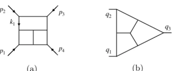
p

₁

p

₂

p

₃

p

₄

k p

₁

p

₂

p

₃

p

₄

k

₁

(a)

q

₁

q

₃

q

₂

Figure 6: (a): Depending on its numerator, the Feynman diagram has different transcenden- (b) tal properties. (b): Off-shell dual conformal Feynman diagram with non-maximal weight.

integrand in N = 4 sYM is essentially contained in on-shell diagrams.

A related way of thinking about on-shell diagrams is that they represent ‘maximal cuts’

of loop integrands, where all loop integrations are replaced by residues. What one obtains in this way are so-called leading singularities of loop integrands. If one thinks of a generic term in an amplitude as r × f , where f is a multi-valued function, and r is some rational or algebraic factor, then the idea is that taking residues of the integrand removes f and leaves us with r. While a quantitative connection is not known, it is expected that the leading singularities describe the factors r that can appear in integrated amplitudes. This knowledge is especially important for bootstrap methods, see section 8.

Leading singularities:

Multi-dimensional residues of loop integrands that localize all integrations.

Thanks to the impressive results above, it became possible to analyze the complete set of four-dimensional loop integrands in N = 4 sYM in detail. It was found that on- shell diagrams can be conveniently described by a mathematical structure called positive Grassmannian (91). This connection allows to classify and evaluate all on-shell diagrams, and to understand identities between them; moreover, their Yangian invariance is manifest.

First studies for general theories include (92, 93).

4.2. Integrands with logarithmic singularities and uniform weight integrals It is useful to extend the notion of transcendental weight of section 2 to functions. This will be done more systematically in the next section, but for now, let us assign weight 1 to the logarithm, and weight −1 to . All evidence to date suggests that L -loop Feynman integrals in four-dimensional QFT evaluate to functions of weight 2L at most. Moreover, scattering amplitudes in N = 4 sYM appear to saturate this bound exactly, i.e. they are conjectured to be uniform weight 2L functions, while amplitudes in QCD have mixed weights 0 ≤ k ≤ 2L . Why is this the case?

It turns out that the answer to the question lies in the loop integrands, i.e. the rational differential forms obtained from writing down Feynman diagrams. Apparently, in N = 4 sYM the Feynman diagrams conspire to give particularly ‘nice’ integrands. To appreciate the point, consider as an example the diagram in Fig. 6(a). This is a particular three- loop Feynman integral obtained from φ

³

vertices. In N = 4 sYM, its contribution to the planar four-particle amplitude comes with a momentum-dependent numerator factor.

In the Lagrangian approach, the latter results from the sum of many Feynman diagrams.

What difference does it make? To see this, let us inspect the first few terms in the Laurent expansion of the integrals in the two theories:

f

sYM

= (−se

^γE

)

⁻³

h

− 1

⁶

16 9 + 1

⁵

13

6 log x + O(

⁻⁴

) i

, 10.

s

²

t

²

f

φ³

= (−se

^γE

)

⁻³

h ₁

⁶

16

9 + 1

⁵

₅ 6x + 8

9 − 13 6 log x

+ O(

⁻⁴

) i

, 11.

where x = t/s, While the N = 4 sYM result has uniform weight 2L = 6, the φ

³

result is a more complicated mixture of weights, with additonal rational dependence on x.

This can be explained by inspecting the loop integrand. The basic idea is that differential forms of the type dτ /τ lead to uniform weight functions, while double or higher poles do not. Note that ‘hidden’ double poles can be revealed by taking (multiple) residues. The integrand of the φ

³

graph of Figure 6 contains double poles, while with the N = 4 sYM numerator it is a 4L -fold dlog differential form. In general, computing leading singularities is an efficient way of testing the uniform weight property. This has been implemented algorithmically (94), and applies to many situations, including non-planar integrals and integrals with massive propagators, which are essential for QCD phenomenology.

One might wonder whether dual conformal symmetry is equivalent to the uniform (and maximal) weight property, but in fact neither implication is true. In the first direction, a counterexample is the three-loop integral shown in Figure 6(b). It is dual conformal, but it evaluates to 20ζ

5

/(q

1²

q

2²

q

²3

) and so does not have maximal weight six. In the second direction, a counterexample is given by the one-loop triangle integral. In fact, it is often even possible to use a basis of uniform weight integrals, see section 5.

THE AMPLITUHEDRON: THE GEOMETRY OF FEYNMAN INTEGRANDS

All evidence to date suggests that loop integrands in N = 4 sYM have only simple poles (95). In the case of planar MHV amplitudes, this statement follows from on-shell recursion relations. The authors of (96) take this further and propose a dual definition of the loop integrand of N = 4 sYM, the Amplituhedron: it is defined as the unique differential form that has logarithmic singularities (i.e. simple poles) only on the boundaries of a certain space related to the kinematics. This remarkable definition does not refer at all to the usual notion of local quantum fields. On the one hand, unlike the Lagrangian formulation, where only conformal, but not dual conformal symmetry is manifest, in this formulation Yangian symmetry is built in.

Moreover, it is free of gauge redundancy. On the other hand, concepts such as unitarity and locality appear as emergent properties.

5. NOVEL METHODS FOR COMPUTING FEYNMAN INTEGRALS

An important problem in perturbative quantum field theory is the following: given some ra- tional loop integrand I , consisting of products of propagators (and possibly some numerator factors coming from the Feynman rules), we would like to carry out the loop integrations,

F(p

i

; ) =

Z d

^D

k

1

. . . d

^D

k

L

(iπ

^D/2

)

^L

I(k

i

, p

j

) , 12.

where k

i

and p

j

are the loop and external momenta, respectively. Typically, the integrals

are regulated by the dimension D = 4−2 , and we are interested in the answer in a Laurent

series around = 0 , which is truncated at some power of . It is useful to think of the answer

as a sum of rational (or algebraic) factors r , and some special functions g , with constant

coefficients c,

F(p

i

; ) = X

k≤2L

X

i,j

c

ijk

1

^k

r

i

g

j

+ O() . 13.

The terms with inverse powers of represent ultraviolet or infrared singularities. In a prac- tical cross-section calculation, the former terms are removed by renormalization, while the latter terms cancel against terms arising from integrating over the phase space of additional emitted particles according to the Bloch-Nordsieck theorem. Here we used the heuristic information that the highest pole in is 2L , and we truncated the expansion at the finite part, which is the physically relevant term. Sometimes higher orders in are needed for consistency of the calculations, or are of genuine interest, for example in the method of expansion near a critical point.

Dimensional regularization: The space-time dimension is taken to be non-integer.

Ultraviolet or infrared divergences appear as poles when the dimension approaches four.

What are the functions g needed in quantum field theory, and specifically for scattering amplitudes? In general, we expect multi-valued functions, since unitarity tells us that amplitudes have discontinuities at thresholds where particles are produced. One can show that, for any one-loop calculation up to O(), the only special functions needed are the logarithm, and one further function, the dilogarithm. They are defined as

log(x) = Z

x

1

dt

t , Li

2

(x) = − Z

x

0

dt

t log(1 − t) . 14.

The dilogarithm has the series representation Li

2

(x) = P

k≥1

x

^k

/k

²

, and we see that Li

2

(1) = ζ

2

. This suggests a generalization of the notion of transcendental weight of section 2. In the context of iterated integrals with logarithmic integration kernels, i.e. of the form d log α, we will call weight the number of iterated integrations, i.e. one for the logarithm, and two for the dilogarithm. This notion naturally generalizes to multiple iterated integrals that appear at higher loop orders.

5.1. Symbol method

Understanding the properties of the special functions appearing in QFT and in particular, their functional identities is very important for a number of reasons. It is desirable to present results in a compact way, making manifest as many (physical) properties as possible. This can be difficult if there are hidden relations between the functions. The same is true when analytically comparing two results from different calculations. Moreover, identities can be used for obtaining representations that are tailored to specific purposes: one representation might be well suited for a series expansion, but perhaps another one is better suited for numerical evaluation.

The dilogarithm and its generalizations satisfy many identities, for example Li

2

(x) + Li

2

(1 − x) + log x log(1 − x) = π

²

6 . 15.

A very useful mathematical tool is the ‘symbol’ (97) of an iterated integral. In a nutshell, it retains the integration kernels in the definition of the iterated integrals, but discards the range of integration. This, together with elementary properties of the d log integration kernels, allows one to easily check equations of the type 15, but also more complicated multi-variable and higher-weight versions of it.

Alphabet: The set of integration kernels, called letters, needed to define classes of iterated integrals.

Key ingredient of the symbol.

Taken together, the set of all integration kernels appearing in a given quantity is called

the alphabet. For example, in the case of Li

2

(x) , it is the set {d log(x), d log(1 − x)} . In

the interest of brevity one often writes only the arguments, i.e. {x, 1 − x}. Knowing the alphabet of a given problem is very important, as it encodes crucial analytic information about the functions. For example, zeros in the alphabet indicate possible, though perhaps spurious, singularities or branch cuts.

The symbol and the notion of alphabet have been used in numerous calculations in N = 4 sYM and QCD. If used appropriately from the outset they guarantee that results are written in a form where the structure of iterated integrals is manifest.

Alternatively, it allows us to find simplifications. As an example, consider the vacuum polarization contribution to the two-loop muon anomalous magnetic moment (98),

Π

^′_γren

(q

²

) =

−α π

!1

0

dz 2z (1

−z) ln(1−z

(1

−z)q²/m²_ℓ

)

=

α π

!1

0

dt t

²

(1

−t²/3)

1

4m

²_ℓ/q²−(1−t²

)

, (73)

and performing the integral yields Π

^′_γren

(q

²

) =

−α

3π

"

8 3

−β²ℓ

+ 1

2

βℓ

(3

−β_ℓ²

) ln

βℓ−

1

βℓ

+ 1

#

, (74)

where

βℓ

=

$

1

−

4m

²_ℓ/q²

is the lepton velocity. The imaginary part is given by the simple formula Im Π

^′_γ

(q

²

) =

α

3

%

1 + 2m

²ℓ

q²

&

βℓ. (75)

For

q²<

0 the amplitude Π

^′_γren

(q

²

) is negative definite and what is needed in Eq. (69) is

−Π^′γ^(ℓ)

(−

_1−x^x2 m²_µ

) or Eq. (74) with

βℓ

=

$

1 + 4

x²_ℓ

(1

−x)/x²

, where

xℓ

=

mℓ/mµ

and

mℓ

is the mass of the virtual lepton in the vacuum polarization subgraph.

Using the representation Eq. (69) together with Eq. (73) the VP insertion was computed in the late 1950s [131] for

mℓ

=

me

and neglecting terms of

O(me/mµ

). Its exact expression was calculated in 1966 [132]

and may be written in compact form as [35]

A⁽⁴⁾2 vap

(1/x)=− 25 36

−

lnx

3 +

x²

(4 + 3 ln

x) +x⁴ 'π²

3

−

2 lnx ln

%

1

x−x

&

−Li2

(x

²

)

(

+

x

2

)

1

−

5x

²*' π²

2

−lnx

ln

%

1

−x

1 +

x

&

−

Li

2

(x) + Li

2

(−x)

(

=− 25 36

−

lnx

3 +

x²

(4 + 3 ln

x) +x⁴ '

2 ln

²

(x)

−

2 lnx ln

% x−

1

x

&

+ Li

2

(1/x

²

)

(

+

x

2

)

1

−

5x

²*'

−lnx

ln

%x−

1

x

+ 1

&

+ Li

2

(1/x)

−Li2

(−1/x)

(

(x > 1)

. (76)

The first form is valid for arbitrary

x. Forx >

1 some of the logs as well as Li

2

(x) develop a cut and a corresponding imaginary part like the one of ln(1−

x). Therefore, for the numerical evaluation in terms of a

series expansion, it is an advantage to rewrite the Li

2

(x)’s in terms of Li

2

(1/x)’s, according to Eq. (A.11), which leads to the second form.

There are two different regimes for the mass dependent effects, the light electron loops and the heavy tau loops [131,132]:

•Light

internal masses give rise to potentially large logarithms of mass ratios which get singular in the limit

mlight→

0

e

a⁽⁴⁾µ(vap, e) = '1

3lnmµ me−25

36+O

%me mµ

&( +α π ,2

.

γ γ

µ γ

Here we have a typical result for a light field which produces a large logarithm ln

^m_m^µ_e ≃

5.3, such that the first term

∼

2.095 is large relative to a typical constant second term

−0.6944. Here the exact 2–loop result

is

a⁽⁴⁾µ

(vap, e)

≃

1.094 258 3111(84)

+α π ,2

= 5.90406007(5)

×10⁻⁶. (77)

30

= x

2 (1 − 5x

²

) h

− log x log _{x − 1}

x + 1

+ Li

2

(1/x) − Li

2

(−1/x) i

| {z }

f₁(x)

− 25 36 − log x

3 + x

²

(4 + 3 log x) + x

⁴

h

2 log

²

x − 2 log x log x − 1

x

+ Li

2

(1/x

²

) i

| {z }

f2(x)

, 16.

where x = m

e

/m

µ

. Physically, this quantity should be single-valued for any value of x > 0 , but we see that individual terms have branch cuts starting at x = 1 . The symbol pro- vides a quick way of verifying that those cuts cancel, and streamlines finding an equivalent expression with better analytic properties. Using identities similar to Equation 15, one finds

f

1

(x) = π

²

4 + 2Li

2

(1 − x) − 1

2 Li

2

(1 − x

²

) , f

2

(x) = π

²

6 + 2 log

²

x + Li

2

(1 − x

²

) . 17.

In this form, the absence of branch cuts for x > 0 is manifest.

The symbol is part of a coproduct structure. The latter helps in systematically keeping track of the integration constants, which are missed by the symbol. We also wish to mention interesting recent work to find a coaction directly at the level of Feynman integrals (99).

Coproduct: Map that decomposes iterated integrals into simpler building blocks.

SYMBOL ALPHABETS AND CLUSTER ALGEBRAS

Perhaps the most striking use of the symbol was the simplification (97) of a previous expression (100) for the two-loop six-gluon MHV amplitude, reducing the size of the final answer from several pages to just a few lines! For this, the observation that the full expression depends on fewer symbol letters than individual terms in the original expression, which suggested the use of a simpler function space. Remarkably, the alphabet identified by (97) turns out to be related to the intriguing mathematical structure of cluster algebras (101). Cluster algebras are a relatively new topic in mathematics, with many fascinating links to topics in mathematics and physics. The connection to the alphabet, and the fact that cluster algebras also appear in the description of the planar loop integrand of N = 4 sYM (91) lends support to the conjecture that this alphabet is sufficient to describe six-gluon amplitudes at higher loop orders, see section 7.

5.2. Canonical differential equations method for computing Feynman integrals In this section we will see that the notion of weight helps in computing Feynman integrals.

Uniform weight integrals satisfy simple differential equations. Let us illustrate this for the