JHEP01(2020)053
Published for SISSA by Springer Received: November 2, 2019 Accepted: December 22, 2019 Published: January 10, 2020
Thermal phase transition in Yang-Mills matrix model
Georg Bergner,a Norbert Bodendorfer,b Masanori Hanada,c Enrico Rinaldi,d,e Andreas Sch¨aferb and Pavlos Vranasf,g
aInstitute for Theoretical Physics, University of Jena, Max-Wien-Platz 1, D-07743 Jena, Germany
bInstitute of Theoretical Physics, University of Regensburg, Universit¨atsstrasse 31, D-93053, Germany
cSchool of Physics and Astronomy and STAG Research Centre, University of Southampton, Southampton, SO17 1BJ, U.K.
dR&D Headquarters, Arithmer Inc., Minato, Tokyo 106-6040, Japan
eInterdisciplinary Theoretical and Mathematical Sciences Program, RIKEN, Wako, Saitama 351-0198, Japan
fNuclear and Chemical Sciences Division, Lawrence Livermore National Laboratory, Livermore, CA 94550, U.S.A.
gNuclear Science Division, Lawrence Berkeley National Laboratory, Berkeley, CA 94720, U.S.A.
E-mail: georg.bergner@uni-jena.de,
Norbert.Bodendorfer@physik.uni-regensburg.de,M.Hanada@soton.ac.uk, enrico.rinaldi@arithmer.co.jp,
Andreas.Schaefer@physik.uni-regensburg.de,vranas2@llnl.gov
Abstract:
We study the bosonic matrix model obtained as the high-temperature limit of two-dimensional maximally supersymmetric SU(N ) Yang-Mills theory. So far, no consensus about the order of the deconfinement transition in this theory has been reached and this hinders progress in understanding the nature of the black hole/black string topology change from the gauge/gravity duality perspective. On the one hand, previous works considered the deconfinement transition consistent with two transitions which are of second and third order. On the other hand, evidence for a first order transition was put forward more recently. We perform high-statistics lattice Monte Carlo simulations at large N and small lattice spacing to establish that the transition is really of first order. Our findings flag a warning that the required large-N and continuum limit might not have been reached in earlier publications, and that was the source of the discrepancy. Moreover, our detailed results confirm the existence of a new partially deconfined phase which describes non- uniform black strings via the gauge/gravity duality. This phase exhibits universal features already predicted in quantum field theory.
Keywords:
Gauge-gravity correspondence, Lattice Quantum Field Theory, M(atrix) The- ories
ArXiv ePrint: 1909.04592
JHEP01(2020)053
Contents
1 Introduction 1
2 Theoretical expectations 5
2.1 Partial deconfinement and possible phase structures
52.2 Large-D, large-N analysis
82.3 Finite-N effects
93 Numerical results 10
3.1 The order of the phase transition and the large-D limit
103.1.1 D = 10 model
113.1.2 D = 26 model
123.2 First order signals from other observables
144 Partial deconfinement 17
5 Conclusion and future directions 20
A Simulation details 25
B Data for N = 32 25
1 Introduction
Bosonic matrix models in one dimension have been studied in various contexts. Despite their simple structure, they display a rich non-trivial phase diagram that can be accessed by analytical methods only in certain limiting cases. An important motivation to study these theories arises from their connections to supersymmetric Yang-Mills theories (SYM) in one and two dimensions, which have various applications to quantum gravity via the gauge/gravity duality [1].
The Euclidean action of the gauged bosonic U(N) matrix model is
1S = N
2λ
Z β0
dt Tr
(D
tX
I)
2−1
2 [X
I, X
J]
2, (1.1)
where λ = g
2YMN is the ’t Hooft coupling, β is the inverse temperature, I, J = 1, 2,
· · ·, d with d = D
−1, and X
Iare N
×N hermitian matrices. The covariant derivative D
tis
1The U(1) part of the gauge group is decoupled from the SU(N) part. Therefore, our results in this paper are valid also for the SU(N) theory. The only technical difference is that the center symmetry becomesZN
instead of U(1). Note also that the U(1) part of the scalars are decoupled. In order to remove the trivial flat direction associated with the U(1) part, we imposeRβ
0 dtXI(t) = 0 for eachI.
JHEP01(2020)053
defined by D
tX
I= ∂
tX
I −i[A
t, X
I], where A
tis the gauge field. We will mainly consider the case D = 10, since it is the bosonic version of the BFSS model [2]. In addition to gauge symmetry, this theory has the U(1) center symmetry. An order parameter associated with the center symmetry is the Polyakov loop,
P = 1
N TrP e
iR0βdtAt, (1.2)
where
Pdenotes the path ordering. The Polyakov loop transforms as P
→e
iθP under the U(1) transformation. Another important symmetry is SO(d) which rotates the X
Iscalars as d-dimensional vectors. In this paper, we will focus on the breaking of the center symmetry.
While the full supersymmetric BFSS model in the large-N limit has a dual gravity description [3], no weakly-curved gravity dual is known for its bosonic part. Still, this model can provide insights into gravity, as we will see shortly. For comparison and to study the large-D limit, we will also investigate the case of D = 26.
This theory is deconfined at high temperature, and confined at low temperature for any D
≥3. Based on large-D and large-N analytical techniques [4] and, partially, on numerical Monte Carlo results at finite N [5], it was initially believed that the deconfinement transi- tion is not a first order one but rather there are two phase transitions, one of second order and one of third order, in close proximity. More recently however, evidence was presented that there may be only one transition of first order [6]. We study numerically the phase diagram of this model in the large-N limit in order to confront the numerical results with analytical predictions, in particular taking into account the continuum limit which was not previously investigated. In this paper, we will provide robust numerical evidence that for D = 10 there is only one deconfinement transition and it is of first order in the large-N limit.
There are several reasons to be interested in the order of the phase transitions for this model. Firstly, let us point out the connection to the topology change between a black hole and a black string [7,
8]. In order to understand it, note that the bosonic matrixmodel in eq. (1.1) is the high-temperature limit of two-dimensional maximally supersym- metric Yang-Mills (SYM) theory compactified on the spatial circle S
1. The bosonic matrix model is obtained by shrinking the temporal circle of the two-dimensional SYM theory to a point. Consequently, what is called the “temporal circle” in the bosonic matrix model actually corresponds to the “spatial circle” in the compactified two-dimensional SYM the- ory. The phase transition we study in this paper is the remnant of center symmetry breaking/restoration along the spatial S
1in this higher-dimensional theory, which can be regarded as the black hole/black string topology change in the
R1,8×S
1spacetime of the dual gravitational description [9].
In the studies of the black hole/black string transition based on general relativity, a
reliable analysis of the topology change is out of reach at the moment due to the unavoid-
able curvature singularity. This problem can be avoided by using the dual gauge theory,
namely the 2d maximal SYM theory mentioned above. The 2d maximal SYM theory con-
tains information about the stringy corrections and can teach us how the singularity can
be resolved. At low temperatures and large N , where the stringy corrections are small, the
dual gravity description predicts a first order transition when the radius of S
1is small [9].
JHEP01(2020)053
Figure 1. Possible phase diagrams of 2d maximal SYM on a circle in the canonical ensem- ble [9, 18]. The vertical axis is the inverse temperature, β = T−1 and the horizontal axis is the radiusR of the spatial circle. The phase transition is related to the breaking of center symmetry along the spatial circle, analogous to confinement and deconfinement. Black hole, uniform black string and non-uniform black string phases on the gravity side correspond to the “completely”
deconfined, confined and “partially” deconfined phases, respectively. (See section 2.1 for the meaning of “complete” and “partial” deconfinement.) Our numerical simulations tell us that the left figure is more likely to be true.
However, the details of how the topology change takes place is out of reach in the gravi- tational approach. At intermediate and high temperatures, the only practical tool to gain insights into the dynamics of the theory is a numerical approach.
Lattice approaches (for example see e.g. refs. [10–13] for recent reviews) are applicable to 2d maximal SYM [14–17]. Numerical approaches are computationally expensive and it is hard to take N sufficiently large at this stage. A theory that is more computationally tractable is the one-dimensional bosonic matrix model eq. (1.1). Depending on the nature of the transition in the bosonic matrix model, the dual gravity prediction of a first order transition may survive at high temperature (left of figure
1), or it may fail and the transitionwill split into two, a third order and a second order one as depicted in the right panel of figure
1. In the former case, we might be able to obtain valuable intuition into the low-temperature region, which is not easy to access with currently available computational resources, from the high-temperature region, which is relatively easier to study. In the latter case, the “non-uniform string” becomes stable due to stringy effects.
Similar problems are of interest in the context of the application of holography to QCD. In fact, this strategy was also used by Witten [19] to study 4d Yang-Mills (YM) as the high-temperature limit of 5d maximal SYM, for which the dual gravity analysis is tractable. Depending on whether the qualitative features of the phase transition change or not, the scope of the holographic
approximationcan change. (See e.g. ref. [20] for detailed discussions regarding this point.) Another example is SYM on
R3×S1deformed by the gaugino mass [21]. The deconfinement transition on a small three-sphere was studied in the same manner [22,
23].The nature of the deconfinement transitions in various gauge theories fits to the frame-
work of partial deconfinement [24] that we will explain in section
2. The matrix modelprovides us with the simplest setup to study it in a non-perturbative way. A good un-
JHEP01(2020)053
derstanding of these transitions might shed light on the deconfinement transition in gauge theories or the microscopic nature of the QCD crossover from the hadronic phase to the quark-gluon-plasma phase.
A related motivation is provided by the black hole information problem. When the phase transition is of first order, there is an unstable phase [24] which is analogous to the Schwarzschild black hole with negative specific heat [25] in the standard setup of the AdS/CFT duality [19]. Therefore, the identification of simple models exhibiting such behavior is the first step towards investigating this issue with a detailed numerical study.
The theory we consider in this paper (eq. (1.1)) admits an analytic treatment in terms of a large-D expansion [4], which predicts two transitions, one of second and one of third order. Numerical Monte Carlo studies at D = 10 [5], up to N = 32, looked consistent with this large-D analysis, while more recent studies [6] for the same value of N seemed to contradict with that analysis.
In the following we investigate some reasons that motivate our investigation. Firstly, finite-N corrections become more relevant near the critical point, in analogy to finite- volume effects of a statistical system near criticality. The numerical data of ref. [5] did not include a dedicated study of finite-N corrections, showing only two values of N . In particular, the transition was studied at N = 32 and we will show that this value is not sufficiently large to reveal the order of the transition by looking at
h|P|i(T ). Other papers [26,
27] which numerically backed up the observation in ref. [5] were not able tostudy the large-N limit either. Evidence for a first order transition was presented in ref. [6], along with a discussion of why the large-D analysis may fail to correctly predict the order of the transition for small D. The first order signal shown in that study was however not completely clear. Moreover, the study did not consider discretisation effects which may affect the nature of the transition by shuffling the order of temperatures if there are multiple transitions as expected from the large-D analysis (see figure
3). This was dueto the limited computational resources available to deal with the considerable increase in numerical cost for larger N and smaller lattice spacing.
Secondly, D = 10 may not be sufficiently large to make contact to the large-D expan- sion and therefore to trust the analytical expectation. In order to get a rough intuition, let us consider an analogous gravity problem, the black hole/black string transition in general relativity on
RD−1×S
1. In this case, the transition is first order at D
≤13 [28] and
large enoughD means D > 13. This suggests that it might be dangerous to trust the large-D analysis at D = 10. Note that the order of the transition is particularly sensitive to the value of D. The large-D analysis seems to be more reliable all the way down to small D for other properties of the theory like the approximate location of the transition [29], see also the dis- cussion in [6]. It is therefore important to study in detail the large-N limit at fixed D = 10.
In this paper, we present numerical evidence that the transition in the D = 10 model is
of first order. Therefore, in figure
1, the left diagrams are more likely to be true. (Although,strictly speaking, our findings also allow for the possibility that the transition is of higher
order at intermediate values of R.) We study D = 26 as well. Somewhat surprisingly, we
have observed signals consistent with a first order transition, which suggests the large-D
approximation is not precise even at D = 26.
JHEP01(2020)053
Figure 2. Matrix representation of the partial deconfinement proposal [24, 30, 31]. The matrix represents a U(M) subgroup of the U(N) gauge group which is ‘deconfined’. Hence the full gauge group is only ‘partially deconfined’.
The organization of this paper is as follows. We start with explaining theoretical expectations in section
2, in order to define the strategy of our numerical simulations.Then, we will show the results of the simulations and their implications in section
3.Section
5is devoted to discussions and conclusions.
2 Theoretical expectations
In this section, we summarize the theoretically expected features of the theory, which will be compared to numerical data and used to determine the order of the phase transition.
We introduce three different patterns characterizing the deconfinement transition [24] and explain how they can be distinguished using numerical simulations. These patterns can be explained by introducing the concept of
partial deconfinement[24,
30, 31]. Since ourmain goal is to identify the order of the transition, we only include relevant details about partial deconfinement and we refer the interested reader to the papers cited above for a comprehensive review.
2.1 Partial deconfinement and possible phase structures
The word ‘partial deconfinement’ [30] is used to characterize a
phasewhere a subset of the U(N ) group, which we denote as U(M ) in the following, is deconfined. A
matrix representationof this concept is illustrated in figure
2. The ‘completely deconfined’ and‘confined’ phases correspond to, as expected, M = N and M = 0, respectively. Intuitively, the reason why partial deconfinement takes place is simpler to understand when working in the large-N limit: complete deconfinement requires an energy of order N
2, and hence, if the energy is much smaller (say E
∼N
2), only a part of the color degrees of freedom can be excited, U(M ) with M
∼ √N . The initial motivation of partial deconfinement was
to understand the gauge theory description of the Schwarzschild black hole with negative
specific heat via the gauge/gravity duality, closely following a very similar mechanism
based on partial Higgs-ing [32,
33] in gauge theories. There have been various consistencyJHEP01(2020)053
checks for several theories, both at weak coupling and strong coupling [24,
30], and explicitdemonstrations based on state counting are available for several theories [34].
In the large-N limit, quite generally, the deconfinement transition in gauge theories was classified in three types [24] according to the picture of canonical ensemble and the concept of partial deconfinement introduced above. Given that there are three phases, we will introduce two temperatures T
1and T
2, the first separating the ‘completely confined‘ and the ‘partially deconfined‘ regions, and the second separating the partially deconfined and the completely deconfined regions. The phase diagram is represented by its absolute value
|P|
as a function of the temperature. In figure
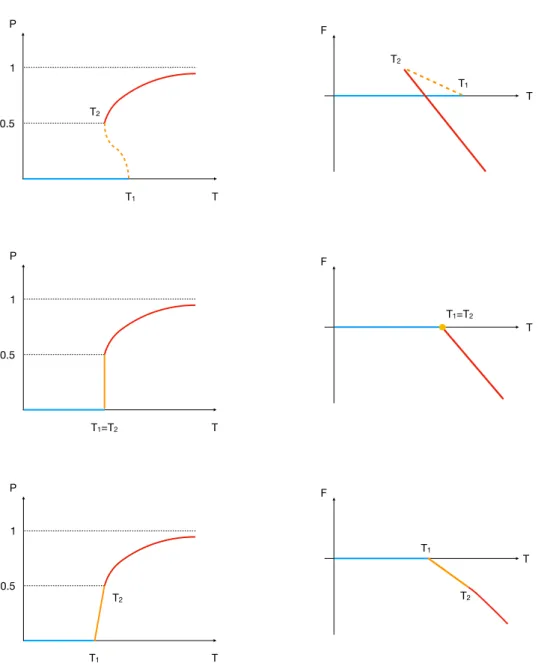
3, the three rows represent the followingthree distinct possibilities for the order of the phase transition:
• First order with hysteresis.
There is a local maximum of the free energy corre- sponding to the partially deconfined phase separating two minima, the completely deconfined phase and the confined phase. A hysteresis sets in at T
2≤T
≤T
1. In the microcanonical ensemble, when the volume is sufficiently large, the confined and com- pletely deconfined phases can occupy most of the space, and the partially deconfined phase appears at the interface. In a matrix model, the partially deconfined phase is stable in the microcanonical ensemble because there are no spatial dimensions and a separation in volume cannot take place.
• First order without hysteresis.
At the transition temperature T = T
1= T
2, there is a Hagedorn string with degenerate free energy [22,
23]. It corresponds to thepartially deconfined phase denoted by the orange line. When the volume is sufficiently large, different vacua can appear at different locations, but this is only realized in systems with spatial dimensions.
• Two transitions of second and third orders.
There are three stable phases with T
1 ≤T
2: even the partially deconfined phase is stable, both in canonical and microcanonical ensemble.
A convenient way to distinguish the three different phases (confined, partially decon- fined and completely deconfined) is to look at the distribution of the phases of the Polyakov loop ρ(θ) [24]. Note that this is just one of the characterizations of the phases. In fact, partial deconfinement does not necessarily require center symmetry, and the Polyakov loop is not necessarily an order parameter for some theories with partial deconfinement [34]. By definition, θ is distributed between +π and
−π. In the confining phase, the distribution isuniform at large N :
ρ
c(θ) = 1
2π . (2.1)
Here, the subscript c stands for ‘confined’. We will use p and d for ‘partially deconfined’ and
‘deconfined’, respectively. The transition between the partially and completely deconfined
phases is the Gross-Witten-Wadia (GWW) transition [35,
36], as found in [24]. Namely,in the partially deconfined phase, the distribution is not uniform, but also not gapped,
i.e. ρ
p(θ) > 0 everywhere in
−π ≤θ
≤π, while in the completely deconfined phase ρ
dis
JHEP01(2020)053
T P
1
0.5
T1
T2
T F
T2
T1
T P
T1=T2
1
0.5
T F
T1=T2
T P
1
0.5
T1
T2
T F
T1
T2
Figure 3. Left: cartoon pictures of the possible phase diagrams of the bosonic BFSS matrix model in the canonical ensemble. In order, the three rows correspond to three deconfinement transitions:
first order with hysteresis (T1 > T2), first order without hysteresis (T1 =T2), and two transitions of second and third orders (T1 < T2). Dashed lines represent unstable phases, while solid lines represent stable or metastable phases. The blue, orange and red lines correspond to the confined, partially deconfined and completely deconfined phases. Right: corresponding free energies for the three types of scenarios. See text for details. Here we use |P|=P.
JHEP01(2020)053
gapped. It is natural to expect [24]
ρ
p(θ) =
1
−M N
·
ρ
c(θ) + M
N
·ρ
GWW(θ), (2.2)
where ρ
GWW(θ) is the distribution at the GWW transition point.
In many cases, the distribution takes a simple form:
ρ
p(θ) = 1
2π (1 + A cos θ) , (2.3)
and
ρ
d(θ) =
A π
cos
θ2q1
A−
sin
2θ2|θ|
< 2 arcsin
q1A
0
|θ| ≥
2 arcsin
q1A
(2.4)
Here, we have fixed the U(1) phase factor using P =
|P|. In the partially deconfinedphase, A = 0 at T = T
1and A = 1 at T = T
2(the GWW transition point), and 0 < A < 1 otherwise. In the transition region, we can interpret A =
MN. In the completely deconfined phase, A
≥1, and M = N regardless of the value of A.
For the bosonic matrix model, the form of ρ
d(θ) in eq. (2.4) has been confirmed by previous studies in a wide region of parameter space [5,
24]. In ref. [5], the form ofρ
p(θ) in eq. (2.3) has also been observed and used as the evidence for the absence of a first order transition. However, as we will see, this is an artifact of the finite-N correction described below in section
2.3.For our purposes it is important to note, for example from figure
3, that in the caseof the first order transition with hysteresis the deconfined phase becomes unstable below P =
12. In other words, if the value of P is stable at 0 < P <
12, the transition cannot be of first order.
2.2 Large-D, large-N analysis
An analytic approach to understanding the thermal phase transition in Yang-Mills matrix models with action eq. (1.1) has been developed in ref. [4]. The key technical tool employed was an expansion of the functional integral around a non-trivial saddle point in the limit of a large number of matrices d (where d = D
−1). Around the saddle point and in this limit, fluctuations are suppressed by powers of 1/d. A priori, it is not obvious what value of d is large enough to justify this expansion, although hints may be obtained from gravity computations, as noted in section
1. Our numerical results suggest thatd = 9 is definitely too small, and even at d = 25 our simulations show a qualitatively different behavior. The analytic agreement with numerical studies [5] mentioned in ref. [4] might be attributed to fact that N
≤32 is too small to reveal the nature of the large-N transition. On the other hand, simulations at N = 32 up to d = 15 were interpreted as consistent with a first order transition [6], in disagreement with the analytical approach.
The results of ref. [4] can be summarized as follows. Throughout the analysis, a gauge
is adopted where A
tis time-independent and diagonal. At low temperatures, the eigenvalue
distribution ρ(θ) of the Polyakov loop P becomes constant as N
→ ∞. As a consequence,JHEP01(2020)053
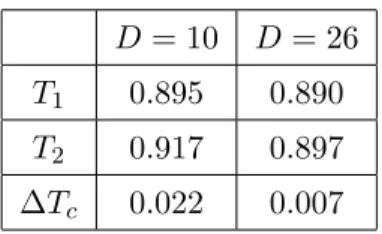
D = 10 D = 26 T
10.895 0.890 T
20.917 0.897
∆T
c0.022 0.007
Table 1. Values ofT1,T2 and their difference ∆Tcfrom eqs. (2.6)–(2.7) withD= 10 andD= 26.
the Polyakov loop vanishes. This behavior persists up to a temperature T
1, where a second order phase transition happens. The large N eigenvalue distribution is now given by
2ρ
T1≤T≤T2(θ) = 1
2π (1 + 2|P
|cos θ) (2.5)
and
|P|continuously increases form 0 to 1/2 as T is increased to a second critical tem- perature T = T
2. With the identification
|P|=
A2=
2NM, this is the same distribution as ρ
pgiven by eq. (2.3). At T = T
2, the third order Gross-Witten-Wadia type [35,
36] phasetransition occurs after which
|P|increases further but with a smaller slope. The eigenvalue distribution becomes gapped at T = T
2and eventually approaches a single delta function at very high temperatures.
The predictions for the critical temperatures including the first 1/d corrections at large N are given by [4]
T
1= d
1/3log d
"
1 + 1 d
203 160
−√
5 3
!#−1
, (2.6)
and 1 T
2 −1
T
1= log d d
4/3"
−
1 6 + 1
d
−
499073
460800 + 203
√5 480
!
log d
−1127
√5
1800 + 85051 76800
!#
. (2.7) We note that for d
→ ∞, ∆Tc:= T
2−T
1 →0, i.e. the two transitions occur in a very narrow temperature regime, making quantitative numerical checks difficult. For the cases considered in this paper, one obtains the values in table
1.2.3 Finite-N effects
By definition, there is no spatial extent in a matrix model. Hence, the thermodynamic limit has to be realized as the large-N limit. The finite-N corrections can obscure the phase transitions, and it is important to know what kind of corrections are expected, in order to determine the nature of the phase transition numerically.
The situation is easier to understand when the large-N transition is not of first order.
Because the large-N limit is the thermodynamic limit, the transition becomes sharper gradually as N increases.
Some caution is required when the large-N transition is of first order. The free energy is of order N
2also in this case, and the fluctuations about the minima are 1/N -suppressed.
2Note that we consider|P|to be normalized to scale asN0.
JHEP01(2020)053
Therefore, at sufficiently large N , the distributions of the observables such as
|P|and E/N
2should have a two-peak structure since tunneling between them is suppressed as e
−const.×N2. However, when N is not sufficiently large, the tunneling probability might be so large that the two peaks merge and become one single wide peak. In this way, the first order nature of the transition gets completely hidden. Even worse, because the confining and deconfining phases give ρ
c(θ) =
2π1and ρ
d(θ) =
2π1(1 + cos θ), the mixture of two phases — say of the confining phase with probability 1
−A and of the deconfining phase with probability A — gives ρ(θ) =
2π1(1 + A cos θ), which is exactly the same as ρ
pof the partially deconfined phase. Therefore, observing a distribution compatible with ρ(θ) =
2π1(1 + A cos θ) is not enough to claim that the transition is not of first order.
3 Numerical results
3.1 The order of the phase transition and the large-D limit
In this section we investigate numerically the phase transition of the bosonic matrix model.
We are in particular interested in the D = 10 case, where the large-D approximation might no longer be applicable. The smooth behavior of the order parameter observed at small N turns into a signal for a transition only in the large-N limit. In this limit, two possible scenarios can be discriminated:
1.
Two distinct transitions become visible:the lower one will be of second order and the higher one will be indicated by an expectation value of the Polyakov loop
h|P|i=
12. Due to the continuous behavior of the Polyakov loop and the small difference of the transition temperatures, the two transitions can only be distinguished at large enough N .
2.
One first order transition appears:in case of the first order transition, the signal will be quite similar to the one of a second order transition. Starting from the low temperature confined phase, there will be a broadening of the minimum of the constraint effective potential and an increase of the susceptibility. However, before the actual second order transition (Hagedorn transition) occurs, a second minimum of the effective potential induces a first order transition.
Because of the nature of this phenomenon, it is difficult to decide about the order of the transition based on the susceptibility, but a two peak signal in the histogram of the order parameter or a hysteresis effect allows a clear distinction of the two scenarios. Therefore, we concentrate on the appearance of these signals at large N in the following investigations.
Our lattice action includes the bosonic part and the gauge fixing part of the BFSS lattice action defined in ref. [37], which was also used in the numerical study of ref. [38].
We consider scans in T at a fixed number of lattice points L and matrix size N . The action
is parameterized in such a way that the lattice spacing scales as 1/L and quantities like
the temperature are all provided in units of the ’t Hooft coupling λ, which is set to unity
in the numerical simulations.
JHEP01(2020)053
● ●
●
●
●
●●
●● ● ●
●
●● ●●
●
●
● ●
●
●
●
●
●
●
●
●
●
●
●
●
●
● ●
● ●● ●●
●
●
●●
●
●
●
●
●
●
●
●
●
●
●
●
● ●
● ●
●
●
● ●●
●
●● ●
●
●
●
●
●
●
●
●
●
●
●
●●
●
●
● ● ●
●
● ● ● ● ●
● ●●
●
● ● ●
● ●
● ●
●
●
●
●
●
●
●
●
●
●
●
●
0.0 0.1 0.2 0.3 0.4 0.5 0.6
0.84 0.85 0.86 0.87 0.88 0.89 0.90 T
|P|
●N=16 ●N=24 ●N=32 ●N=48 ●N=64
(a)
●
●
●
●
●
●
●
●● ●●
●
●
● ●● ●
●
● ●
●
●
●
●
●
●
●
●
● ●
●
●
●
● ●
● ●
● ●●
●
●
●●
●
●
●
●
●
●
●
●
●
●
●
●
● ● ● ● ●
●
● ●●
● ●● ●
●
●●
●
●
●
●
●
●
●
●
●
●
●
●
● ● ● ● ● ● ● ● ●
● ●●● ● ● ●
●
●
● ●
●
●
●
●
●
●
●
●
●
●
●
●
2.18 2.22 2.26 2.30 2.34
0.84 0.85 0.86 0.87 0.88 0.89 0.90 T
R2
●N=16 ●N=24 ●N=32 ●N=48 ●N=64
(b)
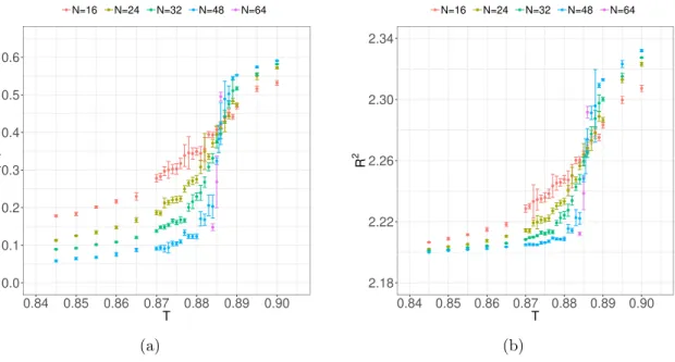
Figure 4. a)|P|vsT and b)R2 vsT, both for L= 24,D= 10 and variousN.
3.1.1 D = 10 model
The first step of our numerical investigation is the measurement of the temperature de- pendence of the expectation value of the Polyakov loop as one approaches the large-N limit. This order parameter will show a smooth behavior at finite N and signal one or two phase transitions in the large-N limit. As shown in figure
4, there are good indications fora transition in the range 0.884 < T < 0.890. This means a rough agreement of T
cwith the predictions of the large-D expansion, but the deviations from large-D predictions are already comparable to ∆T
c=
|T2−T
1|. This indicates that we can not completely rely onthe large-D prediction concerning the realization of one or the other scenario at D = 10.
If we assume the scenario of two separate transitions, the increase of the Polyakov loop would have a finite width ∆T
c, with a rise starting at T
1and stopping at T
2. The slope of
|P|at T
1would increase with N , but the point with
|P|=
12at T
2would remain at a finite distance ∆T
cfrom T
1. Based on this assumptions, we can deduce a rough estimate of
∆T
cand its large-N extrapolation from the width of the transition. At N = 32, which has been the maximal N in previous numerical studies, the obtained width is still compatible with the large-D prediction ∆T
c= 0.022. However, the extrapolation towards the large-N limit does not support a finite ∆T
crequired by the scenario of two separate transitions. In order to substantiate these findings, a more detailed analysis is necessary.
As pointed out above, the best way to discriminate the two scenarios is the two-state
signal or a hysteresis of the order parameter. The two-state signal can be deduced from a
two-peak structure in the histograms of the order parameter that persists in the large-N
limit. In addition, we consider possible effects of the finite lattice spacing by comparing
histograms from simulations with a different number of lattice points L. In case of a first
order transition, the separation of the two peaks becomes more pronounced at large N
since the tunneling rate between the two states is exponentially suppressed with N
2in this
JHEP01(2020)053
limit. The tunneling is also visible in Monte-Carlo time, but this effect is not unambiguous since it has an algorithm dependence.
For N
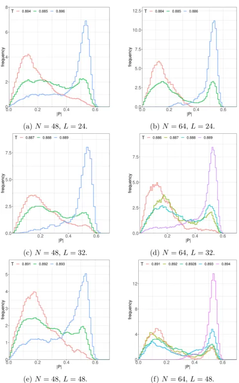
≤32 we can not observe a clear two-peak signal in the histogram (although hints of a two-peak structure are visible, see the appendix), but at N = 48 a two-state signal can be observed that becomes more pronounced at N = 64, see figure
5. There is evidence forthe existence of two phases, one with small
|P|and the other with
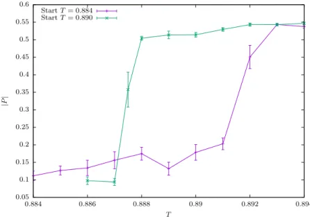
|P| ≈0.5. Consequently, a hysteresis of the order parameter is found, see figure
6. We have investigated threedifferent lattice spacings at N = 64 in order to show that the effect persists in the continuum limit. The complete Monte Carlo history for N = 64, L = 24 is shown in figure
22in the appendix for the transition temperature T = 0.885. It displays repeated tunneling events between the two phases.
Overall, we conclude from these data that there is a first order transition at D = 10 and thus a considerable qualitative deviation from the large-D expansion. However, as figure
7shows, a continuum extrapolation of T
c(which is largely insensitive to N
≥48) would lie within T
1and T
2obtained from the next to leading order expansion in large D. This indicates that at least the location of the transition is correctly estimated by the analytic formulae in section
2.2.Consistent with earlier numerical studies [5], we have seen that the signal at smaller N might indicate a different scenario. We have also found that the peak of the low temperature phase at small
|P|gets significantly broader around the transition temperature. This is consistent with the expected Hagedorn instability at T = T
1. Due to this phenomenon, we observe an increase of the susceptibility towards a peak when approaching the critical temperature from below. Consequently, the first order transition occurs just before a second order transition manifests itself, as anticipated in section
2.1. One would expectthat the transition changes from first to second order at larger D and the picture becomes more consistent with the large-D analysis.
3.1.2 D = 26 model
The analysis of the previous section revealed that the large-D expansion fails to describe the order of the phase transition for D = 10. In this section, we repeat the above investigation for D = 26 which might be large enough for the expansion to be qualitatively applicable, but also small enough to sufficiently limit the computational costs. It turns out that the simulation results are consistent with a first order transition.
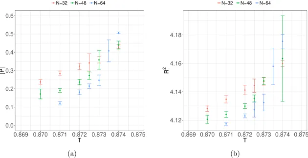
Figure
8shows the dependence of the order parameter
|P|(T) near the transition. A naive large-N extrapolation with fixed lattice size L = 24 locates a possible transition window to be between T = 0.873 and T = 0.874. This separation is much smaller than the predicted width ∆T
c= 0.007 predicted by the large-D expansion (see table
1). Thereis no indication of a finite slope for large values of N . Extrapolating to the continuum using L = 32 and L = 48, indicates that the transition is located close to T
c= 0.89 in the continuum limit, see figure
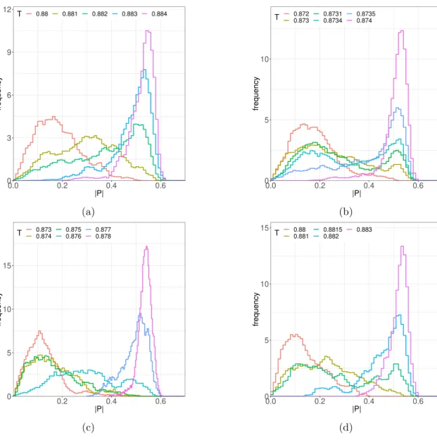
9.Figure
10summarizes the histograms of
|P|for N = 64, L = 24, 32, 48. Compared to
D = 10, the peaks of the distributions are broader, but a two-state signal is still clearly
visible. This is also supported by the Monte-Carlo history, figure
23in the appendix.
JHEP01(2020)053
0 2 4 6 8
0.0 0.2 0.4 0.6
|P|
frequency
T 0.884 0.885 0.886
(a)N = 48,L= 24.
0.0 2.5 5.0 7.5 10.0 12.5
0.0 0.2 0.4 0.6
|P|
frequency
T 0.884 0.885 0.886
(b)N = 64,L= 24.
0.0 2.5 5.0 7.5
0.2 0.4 0.6
|P|
frequency
T 0.887 0.888 0.889
(c)N = 48,L= 32.
0.0 2.5 5.0 7.5
0.2 0.4 0.6
|P|
frequency
T 0.886 0.887 0.888 0.889
(d)N = 64,L= 32.
0 1 2 3 4 5
0.0 0.2 0.4 0.6
|P|
frequency
T 0.891 0.892 0.893
(e)N = 48,L= 48.
0 4 8 12
0.0 0.2 0.4 0.6
|P|
frequency
T 0.891 0.892 0.8928 0.893 0.894
(f)N = 64,L= 48.
Figure 5. Histogram of the order parameter|P|close to the transition temperature for theD= 10 theory.
JHEP01(2020)053
0.05 0.1 0.15 0.2 0.25 0.3 0.35 0.4 0.45 0.5 0.55 0.6
0.884 0.886 0.888 0.89 0.892 0.894
|P|
T StartT= 0.884
StartT= 0.890
Figure 6. Hysteresis cycle for the order parameter|P|withN = 64,L= 32 in theD= 10 theory.
●
●
●
0.0000 0.0005 0.0010 0.0015 0.0020
0.8850.8950.9050.915
1 L2 Tc
●
●
●
● Simulation largeD: T1
largeD: T2
Figure 7. Values forTcextracted from the two-peak histograms extrapolated to the large-N limit for various values ofL. On the left, we show the continuum results from the next-to-leading large-D expansion atD= 10.
3.2 First order signals from other observables
It is useful to study other quantities in order to provide further evidence for the existence or absence of a first order transition. Let us consider
NE2=
−4N3Tr[X
I, X
J]
2and R
2 ≡1 N
Pd
I=1
TrX
I2. If the transition is of first order, the two-peak signal should be visible for these observables as well.
In figure
11and
12we plot the distribution of
NE2and R
2for D = 10. Like for the order
parameter, we observe a first order signal from a clear two-peak structure. Note that the
JHEP01(2020)053
●
●
●
●
●
●
●
●
●
●
●
●
●
●
●
●
●
●
0.0 0.1 0.2 0.3 0.4 0.5 0.6
0.869 0.870 0.871 0.872 0.873 0.874 0.875 T
|P|
●N=32 ●N=48 ●N=64
(a)
●
●
●
●
●
●
●
●
●
●
●
●
●
●
●
●
●
●
4.12 4.14 4.16 4.18
0.869 0.870 0.871 0.872 0.873 0.874 0.875 T
R2
●N=32 ●N=48 ●N=64
(b)
Figure 8. a) |P| vsT and b) R2 vsT, both forL= 24, D= 26 and variousN. A naive large-N extrapolation of|P|is consistent with zero within errors forT ≤0.873 (using data forN= 48 and N = 64 only near the transition).
●
●
●
0.0000 0.0005 0.0010 0.0015 0.0020
0.8750.8800.8850.8900.8950.900
1 L2 Tc
●
●
●
● Simulation largeD: T1
largeD: T2
Figure 9. Values forTcextracted from the two-peak histograms extrapolated to the large-N limit for various values ofL. On the left, we show the continuum results from the next-to-leading large-D expansion atD= 26.
JHEP01(2020)053
0 3 6 9 12
0.0 0.2 0.4 0.6
|P|
frequency
T 0.88 0.881 0.882 0.883 0.884
(a)
0 5 10
0.0 0.2 0.4 0.6
|P|
frequency
T 0.8720.873 0.87310.8734 0.87350.874
(b)
0 5 10 15
0.2 0.4 0.6
|P|
frequency
T 0.8730.874 0.8750.876 0.8770.878
(c)
0 5 10 15
0.0 0.2 0.4 0.6
|P|
frequency
T 0.880.881 0.88150.882 0.883
(d)
Figure 10. Histograms of|P|forD= 26: a)N = 48,L= 48, b-d) N= 64,L= 24,32,48.
locations of the two peaks do not move significantly as a function of N . This is consistent with the theoretical expectation that the maximum of the free energy (partially deconfined phase), rather than the minima (completely deconfined or confined phases), moves.
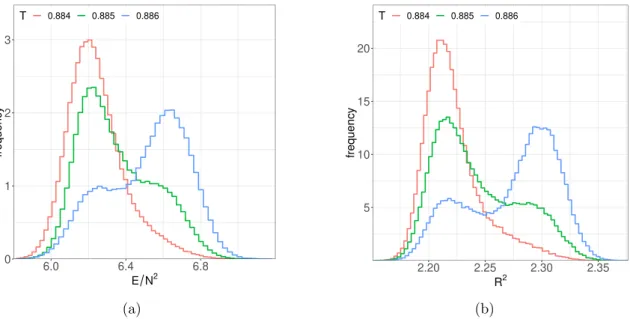
The first order signal from E/N
2and R
2is less pronounced at D = 26, as shown in figure
13for N = 64. We have only presented R
2since the histograms of E/N
2are similar.
For N = 48, no clear signal can be observed, but for N = 64, a two-peak structure is visible.
It is the clearest for L = 24, where we collected higher statistics. The results for L = 48
suggest that the two-peak signal persists in the continuum limit. This is also supported by
the Monte Carlo history shown in figure
23of the appendix. The separation of the phases at
D = 26 is less pronounced compared to D = 10, which might be consistent with the transi-
tion developing towards a combination of higher order transitions at some critical D > 26.
JHEP01(2020)053
0 1 2 3
6.0 6.4 6.8
E N2
frequency
T 0.884 0.885 0.886
(a)
5 10 15 20
2.20 2.25 2.30 2.35
R2
frequency
T 0.884 0.885 0.886
(b)
Figure 11. N = 48,L= 24,D= 10: a) binnedE for variousT. b) binnedR2 for variousT.
0 2 4 6
6.00 6.25 6.50 6.75 7.00
E N2
frequency
T 0.884 0.885 0.886
(a)
0 10 20 30
2.20 2.25 2.30 2.35
R2
frequency
T 0.884 0.885 0.886
(b)
Figure 12. N = 64,L= 24,D= 10: a) binnedE for variousT. b) binnedR2 for variousT.
4 Partial deconfinement
In the previous section, we have determined the order of the deconfinement phase transition.
Let us go one step further and study details of the phase transition. In particular, we use our numerical data to test the partial deconfinement [24,
30,31], reviewed in section2.Partial deconfinement is the proposal that the deconfinement transition happens grad-
ually so that at an intermediate stage only M < N color degrees of freedom are deconfined
(figure
2). We will now derive some consequences of this assumption for correlations be-tween different observables and the eigenvalue distribution of the Polyakov loop, and test
them against our numerical data.
JHEP01(2020)053
0 10 20 30
4.08 4.12 4.16 4.20
R2
frequency
T 0.8720.873 0.87310.8734 0.87350.874
(a)
0 10 20 30 40
4.20 4.25 4.30
R2
frequency
T 0.880.881 0.88150.882 0.883
(b)
Figure 13. Histograms ofR2forN = 64,D= 26 for variousT: a) L=24, b) L=48.
T M
N
T1
T2
0
Figure 14. In the theories with a first order phase transition, there is an unstable saddle (maximum of the free energy) with negative specific heat in the canonical ensemble. In this phase, the SU(M) subgroup of the SU(N) gauge group is deconfined. This phase connects two stable phases, the confining phase (blue line) and the completely deconfining phase (red line).
JHEP01(2020)053
As we have seen, the phase transition is of first order. Then the size of the deconfined sector M should change with temperature as visualized in figure
14. At finiteN , there are non-negligible fluctuations around the saddles, and hence, the size of the deconfined sector M fluctuates configuration-by-configuration during the Monte Carlo simulation. Below, we will relate the value of M to observables (Polyakov loop P , energy E and the extent of space R
2). This leads to nontrivial relations between observables, which can be used for the consistency check of the partial deconfinement proposal. Then we will confirm those relations numerically.
Let us assume that eq. (2.3) holds, at least approximately, at finite N . By using
M
N
= 2|P|, we rewrite eq. (2.3) as
ρ
P(θ) = 1
2 (1 + 2|P
|cos θ) . (4.1)
This relation can easily be tested with our numerical data of the Polyakov phase distribution once the configurations are separated according to their value of
|P|= P . We have plotted the distribution ρ
P(θ) for each bin of
|P|in figure
15obtained from the ensemble at N = 64, L = 24, T = 0.885. The parameters have been chosen to be at the point where the two- state signal indicates a first order transition. Thus our numerical data provides reasonable evidence that eq. (4.1) holds. This shows two things: first, the partial deconfinement prediction eq. (4.1) of superposed eigenvalue distributions holds. Second, the perturbative form of ρ
d(θ) [22,
23] seems to hold (within errors) also in the strongly coupled regime.Since eq. (4.1) holds, it is reasonable to assume partial deconfinement with
MN= 2|P
|.Consequently the partial deconfinement proposal provides further nontrivial predictions:
1. At fixed temperature, the energy per excited degree of freedom is fixed, and hence the energy above the ground state is proportional to M
2. Therefore, as a function of
|P|
and T , we expect
E(|P
|, T)
N
2= ε
0+ f(T)
· |P|2, (4.2)
where ε
0represents the zero-point energy. We expect that this relation is precise at large N , where the fluctuation about the planar limit is suppressed.
2. The same counting holds for R
2 ≡ N1 PdI=1
TrX
I2. Intuitively,
g21 YM|XIij|2
= N
|XIij|2corresponds to the number of open strings excited between i-th and j-th D-branes, which is a function of T. Therefore, N
PdI=1
TrX
I2should be of order M
2, plus the zero-mode contribution which is proportional to N
2. Hence we expect
R
2(|P
|, T) = R
20+ g(T )
· |P|2, (4.3) where R
20comes from the zero-point fluctuation.
Our data confirm these relations with good precision. We provide the data for D = 10 since the results for D = 26 are similar.
As a first check, we have plotted the density distribution of the configurations in
(E,
|P|)-plane in figure16. We have introduced bins in (E,|P|)-plane, counted the numberJHEP01(2020)053
0.0 0.1 0.2 0.3
−3 −2 −1 0 1 2 3
θ
ρ ( θ )
P
0.01 0.1 0.2 0.3 0.4 0.5
Figure 15. Distribution of Polyakov loop eigenvalues compared to the partial deconfinement prediction (black lines) for different P values, where ρP(θ) is defined in eq. (4.1). The Polyakov loop eigenvalues are binned around the indicated value of P with width 0.01.
of configurations in each bin, and repeated the same for R
2as well. As expected, the distribution becomes sharper as N increases due to suppression of fluctuations in the planar limit. This confirms, at least at a qualitative level, that (4.2) and (4.3) are valid.
In order to confirm (4.2) and (4.3) quantitatively, we separate the configurations into bins according to their
|P|value. In that way we obtain expectation values
hEi(|P|, T) of the energy E for fixed
|P|and in the same way
hR2i(|P|, T). Figure
17shows the plot of
1
N2hEi(|P|, T
) as a function of
|P|. We can see very good agreement with (4.2) and (4.3).In ref. [37], the correlation between energy and Polyakov loop in the D0-brane matrix model has been studied in a parameter region with
|P|&0.7, i.e. in the completely decon- fined phase. It was found that the energy and Polyakov loop are not correlated at all. In contrast, we find that even for T = 1.5 where
|P| ≈0.9,
E/N
2and
R
2are correlated, see figure
18. We also studied the low temperature phase atT = 0.5, where there appears to be no correlation.
5 Conclusion and future directions
In this paper, we have studied the nature of deconfinement in the bosonic Yang-Mills matrix model (1.1). We have concluded that the transition is of first order for D = 10.
By interpreting this model as the high-temperature limit of 2d maximal super Yang-Mills (SYM) it is natural to conclude that the phase diagram of 2d maximal SYM is like the left panel of figure
1. Via the gauge/gravity duality, we can rephrase this finding [9] to say thatthe α
0-corrections (which become more important at higher temperatures) do not alter the order of the phase transition between black hole and black string in canonical ensemble.
We have also observed a first order transition for the D = 26 case, which provides
further insights about the validity of the large-D expansion. In comparison with the results
JHEP01(2020)053
5.5 6.0 6.5 7.0
0.0 0.2 0.4 0.6
|P|
EN2
300 600 900 count
(a)
5.5 6.0 6.5 7.0
0.0 0.2 0.4 0.6
|P|
EN2
250500 7501000 1250 count
(b)
6.00 6.25 6.50 6.75 7.00
0.0 0.2 0.4 0.6
|P|
EN2
500 1000 1500 count
(c)
2.20 2.25 2.30 2.35
0.0 0.2 0.4 0.6
|P|
R2
500 1000 count
(d)
Figure 16. (a-c) Correlations ofE/N2and|P|forL= 24,N = 32,48,64 atT = 0.883,0.885,0.885.
d) Correlations ofR2 and|P|forL= 24,N = 64 atT = 0.885.
![Figure 1. Possible phase diagrams of 2d maximal SYM on a circle in the canonical ensem- ensem-ble [9, 18]](https://thumb-eu.123doks.com/thumbv2/1library_info/3728353.1508373/4.892.229.668.135.312/figure-possible-phase-diagrams-maximal-circle-canonical-ensem.webp)
![Figure 2. Matrix representation of the partial deconfinement proposal [24, 30, 31]. The matrix represents a U(M ) subgroup of the U(N ) gauge group which is ‘deconfined’](https://thumb-eu.123doks.com/thumbv2/1library_info/3728353.1508373/6.892.338.537.139.303/figure-matrix-representation-deconfinement-proposal-represents-subgroup-deconfined.webp)