Higher Point Spin Field Correlators in D = 4 Superstring Theory

Higher Point Spin Field Correlators in D = 4 Superstring Theory

D. H¨artl, O. Schlotterer, and S. Stieberger

Max–Planck–Institut f¨ur Physik Werner–Heisenberg–Institut

80805 M¨unchen, Germany

Abstract

Calculational tools are provided allowing to determine general tree–level scattering amplitudes for pro- cesses involving bosons and fermions in heterotic and superstring theories in four space–time dimen- sions. We compute higher–point superstring correlators involving massless four–dimensional fermionic and spin fields. In D = 4 these correlators boil down to a product of two pure spin field correlators of left– and right–handed spin fields. This observation greatly simplifies the computation of such cor- relators. The latter are basic ingredients to compute multi–fermion superstring amplitudes in D= 4.

Their underlying fermionic structure and the fermionic couplings in the effective action are determined by these correlators.

MPP–2009–140

Contents

1 Introduction 4

2 Review of lower order correlators 6

3 From Ramond spin fields to Neveu–Schwarz fermions 9

3.1 Eliminating NS fermions . . . 10

3.2 Factorizing spin field correlators . . . 10

4 Group theoretical background 12 5 Pure spin field correlators 14 5.1 Four–point, six–point and eight–point spin field correlators . . . 14

5.2 The generalization to 2M spin fields . . . 16

6 Explicit examples with more than four spin fields 17 6.1 Five–point functions . . . 17

6.2 Six–point functions . . . 18

6.3 Seven–point functions . . . 19

6.4 Eight–point functions . . . 21

7 Correlation functions with two spin fields 25 7.1 The six– and seven–point function with two spin fields . . . 26

7.2 The n–point correlators with two spin fields . . . 28

8 Manifest NS antisymmetry in correlation functions 30 8.1 Lower order examples . . . 31

8.2 Generalization to n NS fields . . . 33

9 Concluding remarks 34 A Sigma matrix identities 35 A.1 The Lorentz generators and symmetric bispinors . . . 35

A.2 Spin field correlation functions and Fierz identities . . . 36

A.3 Five- and six–point functions . . . 37

A.4 Seven–point functions . . . 38

A.5 Eight–point functions . . . 39 B Ordering and antisymmetrizing sigma matrix chains 42

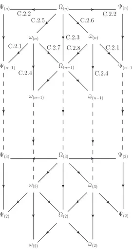
C The n–point correlators with two spin fields: proof by induction 44 C.1 An auxiliary correlator: 2n NS fields . . . 45 C.2 The web of limits . . . 45 D Manifest NS antisymmetry in n–point correlators with two spin fields 57 D.1 Antisymmetrized versus ordered products of sigma matrices . . . 57 D.2 The proof for the antisymmetric representation of Ω_(n),ω_(n) . . . 58

1 Introduction

Multi–parton superstring amplitudes are of both considerable theoretical interest in the framework of a full–fledged superstring theory [1, 2, 3, 4] and of phenomenological interest in describing the scattering processes underlying hadronic jet production at high energy colliders [5, 6]. The key ingredient of these scattering amplitudes is the underlying superconformal field theory (SCFT) governing the interactions of massless string states on the string world–sheet.

In four space–time dimensions this SCFT splits into an internal part and a space–time part. In the low–energy effective action the latter determines the appropriate space–time Lorentz structure of the interactions, while the internal part describes the internal degrees of freedom subject to the underlying compactification [7].

In the (manifestly covariant) RNS fermionic string the space–time part of this SCFT comprises the D = 4 matter fields X^µ, ψ^µ, µ = 0, . . . ,3, (covariant) spin fields S_α, S_β˙, α,β˙ = 1,2, ghost– and superghost system. The Neveu–Schwarz (NS) fermionic fields ψ^µ carry a space–time vector index µ and the Ramond (R) spin fieldsSα, Sβ˙ carry spinor indicesα,β˙ under the Lorentz group SO(1,3). In the RNS formalism the fermionic coordinate fieldsψ^µ of the two–dimensional world–sheet theory are related to the bosonic coordinate fields X^µ through world–sheet supersymmetry. On the other hand, the spin fieldsS_α, S_β˙ convert the fermionic boundary conditions, i.e. intertwine the NS and R sectors.

Their effect on the string world–sheet is the opening and closing of a branch cut [8].

The fermion fields ψ^µ and S_α, S_β˙ enter the massless vertex operators of bosons and fermions, respectively. For concreteness, let us display the vertex operators of a gauge vector multiplet inD= 4 type I superstring theory. The gauge vectorA^a_µ is created by the following vertex operator

V_A⁽⁻¹⁾a (z, ξ, k) = g_AT^a e^−φ(z) ξ^µ ψ_µ(z) e^ikρXρ(z) , (1.1) withφthe scalar bosonizing the superghost system,ξ^µthe polarization vector of the gauge boson and some normalizationg_A. Furthermore,T^aare the Chan–Paton factors accounting for the gauge degrees of freedom of the two open string ends. On the other hand, the vertex operator of the gauginosλ^a, λ^a of negative and positive helicity are given by

V_λ^(−1/2)_a,I (z, u, k) = g_λ T^a e^−φ(z)/2 u^α S_α(z) Σ^I(z) e^ikρXρ(z) , V^(−1/2)

λ^a,I (z,u, k) =¯ gλ T^a e^−φ(z)/2 uβ˙ S^β˙(z) Σ^I(z) e^ikρXρ(z) , (1.2) respectively. Above u^α, u_β˙ are chiral spinors satisfying the on–shell constraints /ku = /ku = 0 and g_λ is a normalization constant. The index I labeling gaugino species may range from 1 to 4, depending on the amount of supersymmetries, while the associated world–sheet fields Σ^I of conformal dimension 3/8 belong to the Ramond sector of internal SCFT [7].

The world–sheet field theory is completely described by giving all correlation functions. Since X^µ, ψ^µ are free fields and the spin fields S_α, S_β˙ are interacting fields the only non–trivial correlators are then+m–point CFT correlators

hψ^µ1(z1). . . ψ^µn(zn)Sα1(x1). . . Sαr(xr)Sβ˙1(y1). . . Sβ˙s(ys)i (1.3) involvingnNS fermionic fields and m=r+sR spin fieldsS_α, S_β˙ with space–time spinor indices α,β˙. Since the covariant spin field Sα is an interacting and double–valued field correlators of several spin fields cannot be computed by using Wick’s theorem and the underlying correlators as (1.3) have to be determined by first principles. Basically, these correlators are completely specified by their properties under theSO(1,3) current algebra of the RNS fermions and their singularity structure [8, 9, 10]. Indeed these correlators can be constructed by analyzing their Lorentz and singularity structure. The latter is dictated by the relevant operator product expansion (OPE) of the fields in the correlators.

The calculation of fermionic string scattering amplitudes requires computing correlators of spin fields Sα, Sβ˙ and fermions ψ^µ. Hence, correlators of the type (1.3) are key ingredients entering the computation of multi–parton superstring amplitudes. Their underlying fermionic structure and the fermionic couplings in the low–energy effective action is revealed by the Lorentz structure of the CFT correlator (1.3).

One of the main observation in this work is, that any correlator of the form (1.3) may be first reduced to a 2n+m–point correlator involving only spin fields Sα and Sβ˙ by replacing each fermion ψ^µ by a pair of spin fields Sα, Sβ˙. Moreover, in D = 4 a correlator involving only spin fields Sα and Sβ˙ factorizes into products of two independent correlators of pure spin fields of one helicity

hS_κ1(z1). . . S_κn(zn)S_α1(x1). . . S_αr(xr)i , hSκ˙1(z1). . . Sκ˙n(zn)Sβ˙1(y1). . . Sβ˙s(ys)i ,

(1.4)

respectively. Hence, for any integersn, mthe correlator (1.3) may be described by products of the two pure spin field correlators (1.4) involving n+r andn+sspin fields of opposite helicity, respectively.

To compute fermionic processes with many external states one generically needs CFT correlators (1.3) for large integers m and n. The purpose of this work is to present the calculational tools and results necessary to compute correlators (1.3) for any m and n. The latter enter the computation of general tree–level scattering amplitudes both in heterotic and superstring theory.

Covariant computation of fermion amplitudes in the RNS model has been advanced at tree–level inD= 10 in [11, 8, 9, 12] at the four–point level, while fermionic amplitudes in D= 10 up to the six–

point level are pioneered in [10, 13]. In D= 4 superstring compactifications multi–parton amplitudes involving many bosons and some fermion fields have been recently computed at disk tree–level [2, 3, 6], see also Refs. [14, 15, 4].

In four–dimensional superstring theories, which preserve at least N = 1 spacetime supersymmetry, it is possible to evade the problem of an interacting CFT by using the hybrid formalism instead of the RNS approach to superstring theory [16]. This formalism is based on some non–trivial field redefinitions, which replace the interacting RNS fieldsψ^µ, S_α and S_β˙ by a new set of free world–sheet fields such that tree–amplitudes are completely fixed by appropriately summing their OPE singularities.

The organization of this work is as follows. In Section 2 we review the CFT of fermion and spin fields and list some basic CFT correlation functions involving fermion and spin fields. In Section 3 we describe how a general correlator of the form (1.3) may be reduced to pure spin field correlators (1.4). In Section 4 we give some group theoretical background allowing to classify and keep track of the Lorentz structure of the correlators (1.3). Moreover, we present a class of vanishing correlators, which give rise to non–trivial consequences for the full string amplitudes in which those enter. In Section 5 we determine the basic correlators (1.4) for any numbers r, s of spin fields. Equipped with these results in Section 6 we compute five– through eight–point correlators (1.3), i.e. n+m= 5, . . . ,8 and display their explicit expressions. The last two Sections 7 and 8 contain closed formulae for correlation functions with two spin fields and an arbitrary number of NS fermions. In Section 7 a basis of ordered products of sigma matrices is used for these correlators, while Section 8 expresses them in terms of antisymmetrized products. In Appendix A and B we present various σ–matrix identities in D = 4.

The latter are needed to simplify correlators and to verify consistency checks of our results. Appendix C and D contain the proofs of the expressions for the two spin field correlators presented in Sections 7 and 8.

2 Review of lower order correlators

In this Section we review the basic OPEs and some correlators of fermionicψ^µ and spin fields Sα. The short distance behaviour of the vector fields ψ^µ from the NS sector and the left- and right- handed spin fields Sα, Sβ˙ from the R sector is governed by the following OPEs

ψ^µ(z)ψ^ν(w) = η^µν

z−w + . . . , (2.1a)

Sα(z)Sβ˙(w) = 1

√2 (z−w)⁰σ^µ

αβ˙ψµ(w) + . . . , (2.1b) S^α˙(z)S^β(w) = 1

√2 (z−w)⁰σ¯^µαβ˙ ψµ(w) + . . . , (2.1c) Sα(z)S_β(w) = −(z−w)^−1/2ε_αβ + . . . , (2.1d) Sα˙(z)Sβ˙(w) = + (z−w)^−1/2ε_α˙β˙ + . . . , (2.1e)

and:

ψ^µ(z)Sα(w) = + 1

√2 (z−w)^−1/2σ^µ

αβ˙S^β˙(w) + . . . , (2.2a) ψ^µ(z)S^β˙(w) = + 1

√2 (z−w)^−1/2σ¯^µβα˙ Sα(w) + . . . . (2.2b) The consistency of these OPEs is easily verified: Eqs. (2.1a) and (2.1b) require that the the OPEs of alike spin fields must differ by a relative sign. If we take the sign convention as in (2.1d) and (2.1e) the OPEs (2.2) are fixed.

One possible way to calculate correlation functions involving NS fermions and R spin fields is by applying all possible OPEs (2.1) and (2.2). Then we can match the terms from the different limits zi→zj to obtain the final result. In the case of the three-point function

hψ^µ(z1)Sα(z2)Sβ˙(z3)i ∼















σ^µ_αγ˙hS^γ˙(z2)Sβ˙(z3)i

√2z₁₂^1/2 = σ^µ

αβ˙

√2 (z12z₂₃)^1/2 forz1 →z2 , σ^ν

αβ˙hψ^µ(z1)ψ_ν(z3)i

√2 = σ^µ

αβ˙

√2z13

forz2 →z3 ,

(2.3)

this method yields

hψ^µ(z1)S_α(z2)Sβ˙(z3)i = σ^µ

αβ˙

√2 (z12z₁₃)^1/2 , (2.4)

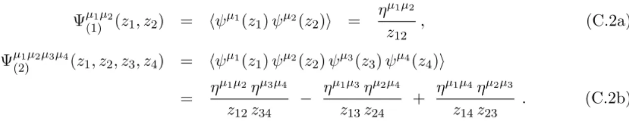
withz_ij :=z_i−z_j. This way further correlators involving two spin fields have been calculated in [2]:

hψ^µ(z1)ψ^ν(z2)S_α(z3)S_β(z4)i = −1

(z13z₁₄z₂₃z₂₄z₃₄)^1/2

η^µνε_αβ z₁₃z₂₄ z12

+ (σ^µσ¯^νε)αβ

z₃₄ 2

, (2.5a) hψ^µ(z1)ψ^ν(z2)S_α˙(z3)Sβ˙(z4)i = + 1

(z13z14z23z24z34)^1/2

η^µνε_α˙β˙

z13z24

z₁₂ + (εσ¯^µσ^ν)_α˙β˙

z34

2

. (2.5b) In [2] the four–point amplitude of one vector, two gauginos and one scalar is derived. Its fermionic structure is determined by the correlators (2.6). A more involved five–point amplitude involving three NS fermions and two R spin fields has been worked out in [3]:

hψ^µ(z1)ψ^ν(z2)ψ^λ(z3)Sα(z4)Sβ˙(z5)i = 1

√2 (z14z15z24z25z34z35)^1/2

× z₄₅

2 (σ^µσ¯^νσ^λ)_αβ˙ + η^µνσ_α^λ_β˙ z₁₄z₂₅

z12 − η^µλσ^ν_αβ˙ z₁₄z₃₅ z13

+ η^νλσ^µ

αβ˙

z₂₄z₃₅ z23

. (2.6) This correlator (2.6) enters the computation of the six–point amplitude involving four scalars and two gauginos or chiral fermions [3]. In addition to these cases with only two spin fields also some pure spin field correlators with four spinor indices are known [2]:

hSα(z1)Sβ˙(z2)Sγ(z3)Sδ˙(z4)i = − εαγεβ˙δ˙

(z13z24)^1/2 , (2.7a)

hSα(z1)Sβ(z2)Sγ(z3)Sδ(z4)i = ε_αβε_γδz₁₄z₂₃ − ε_αδε_βγz₁₂z₃₄

(z z z z z z )^1/2 , (2.7b)

hSα˙(z1)Sβ˙(z2)Sγ˙(z3)Sδ˙(z4)i = ε_α˙β˙ε_γ˙δ˙z14z23 − ε_α˙δ˙εβ˙γ˙z12z34

(z12z13z14z23z24z34)^1/2 . (2.7c) These correlators are basic ingredients of four–point amplitudes involving gauginos or chiral matter fermions [2, 5]. To check the individual limits zi → zj of the correlation functions (2.7a)– (2.7c) the z–crossing identity

zijzkl = zikzjl + zilzkj (2.8)

proves to be useful.

Some care is required to incorporate the complex phases which arise upon performing the OPEs.

Since OPEs are defined by the action of the involved fields on the vacuum state |0i, it is necessary to

“shift” the respective fields first to the right end of the correlation function before applying the OPE.

The limit z2 →z3 in (2.5a), for instance, requires to commute ψ^ν(z2)Sα(z3) past Sβ(z4). Due to the fractional powers ofz−win (2.1d) and (2.2a) bothψ^ν andS_α catch a phase ofiwhen they are moved acrossSβ. So an additional minus sign appears

hψ^µ(z1)ψ^ν(z2)S_α(z3)S_β(z4)i = (−1) σ_α^ν_γ˙

√2z₂₃^1/2hψ^µ(z1)S^γ˙(z3)S_β(z4)i + O(z₂₃^1/2), (2.9) which gives the correctz2 →z3 limit of (2.5a) using−σ^ν¯σ^µ= 2η^µν+σ^µσ¯^ν. This relations shows that not all possible index terms are independent. The same thing happens in the case of the correlations functions (2.7b) and (2.7c). Using the Fierz identity

εαγεβδ = εαβεγδ + εαδεβγ (2.10)

one possible index configuration can be eliminated. In Section 4 we systematically study how many independent index configurations exist for a particular correlator.

Determing all correlation functions by considering all possible OPEs only works consistently if all available σ– and Fierz identities are used to reduce the set of index terms to its minimal number.

Finding these identities for higher order correlators is quite involved. Hence, this method is rather inefficient for these cases. In fact, in the next Section we propose a much more efficient way.

Besides, there is an efficient method to compute correlation functions with two fermion fields ψ at coinciding positions by making use of their Lorentz structure. The operators

J^µν(z) := ψ^[µ(z)ψ^ν](z) (2.11)

realize theSO(1,3) current algebra at levelk= 1. Above the brackets [. . .] denote anti–symmetrization in the indices µ, ν. Hence, their insertion into a correlator implements a Lorentz rotation. Any correlator includingJ^µν can be reduced to its relatives with one current insertion less by means of the following prescription [17] (see also [8, 9, 10])

hJ^µν(z)ψλ1(z1). . . ψλn(zn)Sα1(x1). . . Sαr(xr)Sβ˙1(y1). . . Sβ˙s(ys)i

= −

n

X

j=1

2 z−z_j δ^[µ_λ

jhψ_λ1(z1). . . ψ^ν](zj). . . ψ_λn(zn)S_α1(x1). . . S_αr(xr)S_β˙

1(y1). . . S_β˙

s(ys)i

−

r

X

j=1

1

2 (z−x_j) σ^µν_αj^κhψ_λ1(z₁). . . ψ_λn(z_n)S_α1(x₁). . . S_κ(x_j). . . S_αr(x_r)Sβ˙1(y₁). . . Sβ˙s(y_s)i +

s

X

j=1

1

2 (z−y_j) σ¯^µνκ˙β˙jhψ_λ1(z1). . . ψ_λn(zn)Sα1(x1). . . Sαr(xr)Sβ˙1(y1). . . Sκ˙(yj). . . Sβ˙s(ys)i (2.12) as a result of theSO(1,3) action on the relevant fields:

J^µν(z)ψ^λ(w) = − 2

z−w η^λ[µψ^ν](w) + . . . , (2.13a) J^µν(z)Sα(w) = − 1

2 (z−w) σ^µνακSκ(w) + . . . , (2.13b) J^µν(z)S^α(w) = + 1

2 (z−w) σ^µνκαS^κ(w) + . . . , (2.13c) J^µν(z)S^β˙(w) = − 1

2 (z−w) σ¯^µνβ˙κ˙S^κ˙(w) + . . . , (2.13d) J^µν(z)Sβ˙(w) = + 1

2 (z−w) σ¯^µνκ˙β˙Sκ˙(w) + . . . . (2.13e) Note that in case of severalJ^µν insertions the central term of the current–current OPE arises:

J^µν(z)J^λρ(w) = 1

(z−w)² η^µρη^νλ − η^µλη^νρ

+ 1

z−w

η^µλJ^νρ(w) − η^µρJ^νλ(w) − η^νλJ^µρ(w) + η^νρJ^µλ(w)

+ ... . (2.14) As a simple example of this method, let us compute the four point function (2.5a) at z₁ =z₂:

hψ^µ(z1)ψ^ν(z1)Sα(z3)S^β(z4)i = hψ^[µ(z1)ψ^ν](z1)Sα(z3)S^β(z4)i = hJ^µν(z1)Sα(z3)Sβ(z4)i

= − 1

z13

σ^µνακhSκ(z3)S^β(z4)i + 1 z14

σ^µνκβhSα(z3)S^κ(z4)i = −z₃₄^1/2 z13z14

σ^µναβ. (2.15) However, the goal of this article goes far beyond the application of Eq. (2.12). All the correlation functions will be given in full generality without any coinciding arguments. Of course, by a posteriori moving fermion positions together, one can obtain nice consistency checks for the results in the following Sections.

3 From Ramond spin fields to Neveu–Schwarz fermions

After having collected existing results for some lower order correlation functions we now develop a new method to systematically obtain correlators with arbitrarily manyψ^µ andS_α, S_β˙ fields. First we show how NS fermions can be reduced to a product of spin fields. Then it is demonstrated that in

four space-time dimensions the correlation function factorizes into a correlator of right-handed and a correlator of left-handed spin fields.

3.1 Eliminating NS fermions

Let us first look at the D dimensional generalization of the OPE (2.1) of two different spin fields.

Spinor indices of SO(1, D−1) will be denoted by A, B and the corresponding gamma matrices by Γ^µ_AB. Since spin fieldsSA(zi) inDspace-time dimensions have conformal weightD/16, the OPE ofSA

and S_B with appropriate relative chirality (alike in D= 4k+ 2 and opposite inD= 4k) is given by S_A(z)S_B(w) = Γ^µ_AB(z−w)^1/2−D/8ψ_µ(w) + O (z−w)^3/2−D/8

. (3.1)

From the most singular term ∼ (z −w)^1/2−D/8, one can read off the special property in D = 4 dimensions – there is no singularity as z→w:

S_α(z)S_β˙(w) = 1

√2σ^µ

αβ˙(z−w)⁰ψ_µ(w) + O(z−w). (3.2) Settingz=w leaves a non-trivial contribution on the right hand side:

S_α(z)S_β˙(z) = 1

√2σ^µ

αβ˙ψ_µ(z). (3.3)

Making use ofσ_κ^µ_κ˙σ¯^νκκ˙ =−2η^µν this can be inverted:

ψ^µ(z) = − 1

√2σ¯^µκκ˙ S_κ˙(z)S_κ(z) . (3.4) Hence, it is possible to replace all NS fermions in the following correlator:

hψ^µ1(z1). . . ψ^µn(zn)Sα1(x1). . . Sαr(xr)Sβ˙1(y1). . . Sβ˙s(ys)i =

n

Y

i=1

−σ¯^µiκ˙iκi

√2

× hSκ1(z1). . . Sκn(zn)Sα1(x1). . . Sαr(xr)Sκ˙1(z1). . . Sκ˙n(zn)Sβ˙1(y1). . . Sβ˙s(ys)i . (3.5) We see that an arbitrary correlation function can be written as a pure spin field correlator contracted by some σ matrices. The next step is to systematically determine these correlators.

3.2 Factorizing spin field correlators

Looking at the simple result (2.7a) for the four spin field correlation function hSαSβ˙SγSδ˙i one can identify it as the product of the two point functions:

hSα(z1)Sγ(z3)i = − εαγ

z^1/2₁₃ , hSβ˙(z2)Sδ˙(z4)i = εβ˙δ˙

z₂₄^1/2 . (3.6)

We prove now that this factorization property holds for an arbitrary number of spin fields. In order to do this it is most convenient to treat them in bosonized form [10]. The left- and right-handed spin fields in four dimensions can be represented by two boson Hi=1,2(z)

Sα=1,2(z) ∼ e^{±2i[H1(z)+H2(z)]} =: e^{i~p ~H(z)},

Sβ=1,2˙ (z) ∼ e^{±2i[H1(z)−H2(z)]} =: e^{i~q ~H(z)}, (3.7) with vector notation H(z) =~ H₁(z), H2(z)

for the bosons and weight vectors p~ = ±¹₂,±¹₂ , ~q =

±¹₂,∓¹₂

. Note that the weight vectors of distinct chiralities are orthogonal,~p ~q= 0. The two bosons fulfill the normalization convention:

hH_i(z)H_j(w)i = δ_ij ln (z−w). (3.8) Cocycle factors which yield complex phases upon moving spin fields across each other are irrelevant for the following discussion and are therefore neglected.

The OPEs (2.1b)–(2.1e) as well as the four point functions (2.6) can be traced back to:

e^{i~p ~H(z)}e^{i~q ~H(w)} ∼ (z−w)^{p ~~q}e^{i(~p+~q)H~(w)} +. . . , (3.9a) DYⁿ

k=1

e^{i~pkH(z~ k)}E

∼ δ

n

X

k=1

~ pk

! _n Y

i,j=1 i<j

z^~p_ij^ip~j . (3.9b)

Hence the correlation function ofr left-handed ands right-handed spin fields becomes:

hS_α1(z1). . . S_αr(zr)S_β˙

1(w1). . . S_β˙

s(ws)i = DY^r

k=1

e^i~pkH~(zk)

s

Y

l=1

e^i~qlH~(wl)E

= δ

r

X

k=1

~ p_k+

s

X

l=1

~q_l

! _r Y

i,j=1 i<j

z_ij^~pi~pj

s

Y

¯ı,¯=1

¯ ı<¯

w_¯^~q_ı¯^¯ı~q¯

r

Y

m=1 s

Y

n=1

(zm−w_n)^p~m~qn

| {z }

=1

= δ

r

X

k=1

~ p_k

! _r Y

i,j=1 i<j

z_ij^~pi~pj δ

s

X

l=1

~q_l

! _s Y

¯ ı,¯=1

¯ı<¯

w_¯ı¯^~q_^¯ı~q¯ = DY^r

k=1

e^{i~pkH(z~ k)}E DY^s

l=1

e^{i~qlH(w~ l)}E

= hS_α1(z1). . . S_αr(zr)i hS_β˙

1(w1). . . S_β˙

s(ws)i. (3.10)

From the second to the third line we have used that~p_m ~q_n = 0 and theδ-function has been split into the linearly independentp~and~qcontributions. So we see that a general spin field correlation function in four dimensions splits indeed into two correlators involving only left- and right-handed spin fields respectively¹.

1We want to stress that this result does not generalize to arbitrary dimensions. For D = 2k an even number of minus signs has to appear in thek entries of~p, whereas~q must contain an odd number of minus signs. Then fork >2 the crucial property~p ~q= 0 for weight vectors ~p, ~qof opposite chirality used in (3.10) does not hold any longer.