Many-body spin echo

(1)

Many-body spin echo

Thomas Engl,

¹

Juan Diego Urbina,

¹

Klaus Richter,

¹

and Peter Schlagheck

²

1

Institut für Theoretische Physik, Universität Regensburg, D-93040 Regensburg, Germany

2

CESAM Research Unit, University of Liege, 4000 Liege, Belgium

(Received 30 March 2018; published 30 July 2018)

We show that quantum coherence produces an observable many-body signature in the dynamics of few-fermion Hubbard systems (describing cold atoms in optical lattices, coupled quantum dots, or small molecules) in the form of a revival in the transition probabilities echoing a flip of the system’s itinerant spins. Contrary to its single-particle (Hahn) version, this many-body spin echo is not dephased by strong interactions or spin-orbit coupling, and constitutes a benchmark of genuine many-body coherence. A physical picture that allows for the analytical study of this nonperturbative effect is provided by a semiclassical approach in Fock space, where coherence arises from interfering amplitudes associated with multiple chaotic mean-field solutions with action degeneracies due to antiunitary symmetries. The analytical predictions resulting from our semiclassical approach are in excellent quantitative agreement with corresponding numerical simulations. The latter, moreover, confirm that the shape of the echo profile is independent of the interaction, while its amplitude and sign universally depend only on the number of flipped spins and the spin-orbit coupling phase.

DOI: 10.1103/PhysRevA.98.013630

I. INTRODUCTION

Echoes such as the spin (or Hahn) [1], mesoscopic [2], Loschmidt echo [3], and plasma wave echo [4] as well as time-reversal focusing [5] are among the fascinating quantum interference effects that have quickly become an important tool to characterize quantum coherence, stability of quantum dynamics, Anderson localization, and the transition to classical behavior in quantum systems [6–11]. Echo phenomena also provide a way to gather information about many-body systems.

Variations of the basic setup, such as the echo signal of a single degree of freedom coupled to a spin chain [12–14] or the spin echo in a gas of ultracold trapped atoms [15], are subject of present studies and can be used for measuring correlation functions and localization in many-body systems [16,17].

As most of the research on echo phenomena has focused on single-particle observables of many-body systems, interactions and uncontrolled external fields typically dephase the respec- tive single-particle signals. This motivates to study many-body echoes as signatures of the fully coherent many-body quantum dynamics in interacting few-fermion systems. Intrinsic mech- anisms of spin-precession preserving time-reversal invariance are provided by spin-orbit coupling (SOC) [18,19] which can be implemented for ultracold atoms [20]. We describe such systems by the Fermi-Hubbard Hamiltonian

H ˆ =

L

l=1

[

l

( ˆ c

^†_l_↑

c ˆ

_l_↑

+ c ˆ

^†_l_↓

c ˆ

_l_↓

) + U c ˆ

^†_l_↑

c ˆ

_l^†_↓

c ˆ

_l_↓

c ˆ

_l_↑

]

− J

L

l=1

σ=↑,↓

( ˆ c

_lσ^†

c ˆ

l−1,σ

+ c ˆ

^†_l_−1,σ

c ˆ

lσ

)

+ α

L

l=1

[e

^iϕ

( ˆ c

^†_l_↓

c ˆ

l−1↑

− c ˆ

^†_l_−1↓

c ˆ

l↑

) + H.c.] (1)

with periodic boundary conditions (i.e., ˆ c

_0σ

≡ c ˆ

_Lσ

and ˆ c

^†_0σ

≡ ˆ

c

^†_Lσ

for σ = ↑ , ↓), spin-independent onsite energies

l

, the onsite spin-spin interaction U, the spin-preserving nearest- neighbor hopping parameter J > 0, as well as the spin-orbit coupling strength α > 0.

The many-body spin echo (MBSE) protocol, a natural lift of the Hahn echo into the many-body domain, is presented in Fig. 1. Instead of focusing on a single-particle observable (like the spin polarization), we propose to measure transition probabilities between many-body initial and final occupation (Fock) states. After post-selection of states that are related with the initial one by a set of specific antiunitary operations, we predict an echo signature of quantum coherence which is robust with respect to interactions and/or SOC. The cor- responding experimental challenge consists in the preparation and the projective measurement of many-body Fock states with single-particle precision, and in repeating the above protocol sufficiently often in order to achieve significative statistics for the post-selected states. Our simulations of such experiments indicate that a MBSE can already be observed in rather small systems containing four particles on four sites. This can be routinely realized with coupled quantum dots or fermionic cold atoms in optical lattices, where the interaction, hopping, and SOC parameters can be widely tuned and individual particles can be spin-sensitively measured and manipulated [20–41].

II. NUMERICAL FINDINGS

Specifically, as shown in Fig. 1 we consider a system

of N itinerant interacting fermions on a lattice of L sites

in the presence of SOC. Initially, the system is prepared in

an arbitrary Fock state |n = | n

_1↑

, n

_1↓

, . . . , n

L↑

, n

L↓

, where

n

l↑(↓)

∈ {0, 1} denotes the occupation number with spin up

(down) at the lth site. After the system has evolved for some

time t

_F

, the spins of the particles at M L sites are suddenly

(2)

FIG. 1. Protocol of the many-body spin echo. An initial Fock state (bottom line) evolves under the many-body Hamiltonian ˆ H which features orbital and spin dynamics as well as interactions. At time t

F

, when the system is in a superposition of Fock states, part of the spins are flipped. After further propagation for a time t

= t

F

+ τ the occupancies at each site are projectively measured (top line).

reversed through the spin-flip operator ˆ A =

n

|F

^(M⁾

nn|

where the spin-flip matrix F

^(M⁾

= σ

_x⁽¹⁾

× · · · × σ

_x^(M)

with σ

_x^(l)

the x -Pauli matrix acting on site l interchanges the occupancies n

l↑

and n

l↓

within the Fock state |n on all sites 1 l M [42]. The system is then further propagated for a time t

= t

F

+ τ and the probability to obtain the occupancies n

,

P (n

, n; τ ) = |n

| U(t ˆ

F

+ τ ) ˆ A U(t ˆ

F

)|n|

²

(2) with ˆ U(t ) = exp(− it H /¯ ˆ h), is measured as a function of the time mismatch τ . To reveal robust system-independent fea- tures, we perform a configurational average of this probability over an ensemble of random onsite energies

l

.

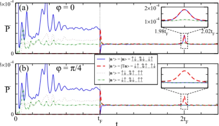
Figure 2 shows as a function of the evolution time t the average probabilities (2) for the initial state |n

= |n, its spin- flipped counterpart |n

= |Tn with T ≡ F

^(L)

, as well as for two other Fock states that exhibit the same one- and two-body onsite energies as the initial state. This numerical simulation was carried out for a Fermi-Hubbard chain of L = 8 sites with U = J and α = 0.2J , using a Lanczos method [43]. We chose a generic initial state |n = |↑ , ↓ , 0, ↑↓ , ↓ , 0, ↓ , ↑ such that we can expect it to be connected to a large ergodic domain for the above interaction and spin-orbit coupling parameters, and performed a disorder average over 10 000 random choices for the onsite energies drawn from a uniform distribution in the interval

l

∈ [0, 2J ] [44].

Until t = t

_F

the average probability to detect the initial state features, as we clearly see in Fig. 2, a factor-2 enhancement as compared to other states with comparable total energy, which is a consequence of coherent backscattering in Fock space [45].

Its spin-flipped counterpart is not detected at all, owing to the existence of a time-reversal symmetry with an antiunitary operator T satisfying T

²

= − 1 on the single-particle level [see Eq. (14) below] which for an odd total number of particles gives rise to a vanishing probability for |Tn. Perfect ergodicity is established after the spin flip taking place at t = t

F

on all sites (i.e., for M = L), where we chose J t

F

= 25 in the numerical simulation. Around t = 2t

F

, however, short-term factor-2 enhancements in the disorder-averaged probabilities are again encountered, in perfect agreement with our analytical prediction (see Sec. III below). Those enhancements occur both for the initial state |n and its spin-flipped counterpart |Tn in the case of real-valued spin-orbit coupling [ϕ = 0, Fig. 2(a)],

FIG. 2. Many-body spin echo in a Fermi-Hubbard ring with 7 particles on 8 sites (a) for real spin-orbit coupling (ϕ = 0) as well as (b) for the SOC phase ϕ = π/4. Plotted is as a function of time the disorder average P of the probability (2) to obtain the final Fock state |n

, for the initial state |n

= |n, its spin-flipped counterpart

| n

= | Tn , as well as for two other final states that are unrelated with |n. Coherent effects that remain for t t

F

are lost after the application of the spin-flip operator ˆ A at time t

F

(with J t

F

chosen to be 25), following the protocol in Fig. 1. At t = 2t

F

, however, the detection probability undergoes a temporary echo enhancement for | n

= | n and | Tn in the case of real SOC (a) as well as for | n

= | Tn only at ϕ = π/4 (b). The calculation was specifically done for the initial state | n = |↑ , ↓ , 0, ↑↓ , ↓ , 0, ↓ , ↑ with the spin-orbit coupling α = J /5, the spin-spin interaction U = J , and the disorder strength

l

∈ [0, 2J ] in units of the nearest-neighbor hopping J, but the key results presented here do not depend on the precise values of these parameters nor on the choice of the initial state [44].

while they concern |Tn only for the spin-orbit coupling phase ϕ = π/4 as seen in Fig. 2(b).

III. SEMICLASSICAL THEORY A. Semiclassical propagator

The occurrence of this MBSE feature can be understood in terms of constructive path interference that arises within the Fock space of the fermionic many-body system under consid- eration. To support this claim, we stress that a semiclassical approximation for the microscopic path-integral propagator of discrete fermionic quantum fields can be derived as shown in Ref. [46] provided one is dealing with a large number N 1 of itinerant fermions. Projected to Fock states, this semiclassical propagator can be expressed as

n

| U ˆ (t )|n

γ:n→n

A

γ

exp(iR

γ

/ h) ¯ (3)

in terms of classical trajectories γ that evolve from n to n

. The latter are constituted by complex multicomponent classical fields

ψ

^(γ⁾

(s ) ≡

ψ

_1↑^(γ⁾

(s ), ψ

_1↓^(γ⁾

(s), . . . , ψ

_L^(γ_↑⁾

(s), ψ

_L^(γ_↓⁾

(s ) (4) that evolve according to Hamilton’s equations

i h ¯ d

ds ψ

_lσ

(s) = ∂

∂ψ

_lσ^∗

H

_mf

[ψ

^∗

(s), ψ (s)], (5)

(3)

generated by a classical (mean-field-like) Hamiltonian H

_mf

[46] whose explicit form will not be relevant in the follow- ing. The solutions fulfill the boundary conditions | ψ

lσ

(0)|

²

= n

lσ

and | ψ

lσ

(t )|

²

= n

_lσ

at the initial and final times, respec- tively, for 0 l L and σ = ↑ or ↓. Introducing the action- angle variables

I

_lσ^(γ⁾

(s) = ψ

_lσ^(γ⁾

(s )

²

, (6) θ

_lσ^(γ⁾

(s ) = arg ψ

_lσ^(γ⁾

(s) (7) for all 0 l L and σ = ↑ , ↓ allows us to express the classical action associated with the trajectory γ as

R

γ

=

t

0

ds

lσ

¯

hθ

_lσ^(γ⁾

(s ) d

ds I

_lσ^(γ⁾

(s) − E

γ

t, (8) where E

γ

= H

_mf

[ψ

^(γ⁾^∗

(0), ψ

^(γ⁾

(0)] is the (conserved) clas- sical energy of the trajectory and A

γ

denotes the associated semiclassical amplitude [46].

The above expression (3) can be straightforwardly gener- alized to incorporate the occurrence of a partial spin flip at t = t

F

. This yields the semiclassical propagator

n

| U ˆ (t

) ˆ A U ˆ (t )|n

m

γ ,γ

A

γ

A

γ

e

^i(R^γ⁺^R^γ^)/¯^h

, (9) where the trajectories γ : n → m and γ

: F

^(M)

m → n

, re- spectively, go from n to m within the time t as well as from F

^(M⁾

m to n

within t

.

B. Diagonal approximation

Since Eq. (5) generically displays chaotic behavior [47], the Bohigas-Giannoni-Schmit conjecture of quantum chaos [48]

predicts the emergence of universal signatures of quantum interference [49] revealed by averages that respect the sym- metries of ˆ H in Eq. (1). Equations (2) and (9) make such in- terferences (between many-body amplitudes) explicit through a coherent fourfold sum over mean-field trajectories

P (n

, n; τ ) ≈

m,m

γ1 :n→m γ3 :n→m

γ2 :F(M)m→n γ4 :F(M)m→n

A

γ1

A

γ2

A

^∗γ₃

A

^∗γ₄

exp

i

^γγ³₁^γγ⁴₂

, (10)

with

^γγ³₁^γγ⁴₂

= (R

γ1

+ R

_γ₂

− R

_γ₃

− R

_γ₄

)/ h ¯ (11) denoting the combined action differences. Large exponents with

^γγ³₁^γγ⁴₂

∝ N 1 give rise to fast oscillations within Eq. (10), which generally cancel out upon average. Exceptions arise only if there are classical correlations between pairs of actions, determined solely by the antiunitary symmetries of the Hamiltonian (1).

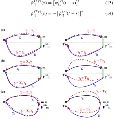
Such correlations trivially occur for the special cases γ

₁

= γ

₃

and γ

₂

= γ

₄

. Restricting the multiple sum in Eq. (10) to the terms that satisfy those conditions constitutes the diagonal approximation, which treats the two propagation steps as independent, as depicted in Fig. 3(a). It yields the classical background

P

_cl

(n

, n; τ ) =

m

p

_cl

(n

, F

^(M⁾

m; t

F

+ τ )

× p

_cl

(m, n; t

F

) , (12) where p

_cl

(m, n; t ) is the classical transition probability be- tween the occupancies n and m at time t . Assuming per- fect ergodicity, the latter is approximately expressed as p

_cl

(m, n; t ) = 1/ N under average where N is the number of Fock states featuring N particles [45] (see Appendix A).

C. Interference contributions

From all other possibilities of trajectory pairing, some re- quire very special conditions on the intermediate occupancies m and m

(such as, e.g., m = m

= n) and thus yield negligible contributions. Neglecting furthermore so-called loop contribu- tions [50–54] leaves us with two more possibilities to get a correlated pair: a trajectory γ , as given by the classical field amplitudes ψ

_lσ^(γ⁾

(s ) that evolve from s = 0 to the final time t ,

can be paired with its time-reversed counterpart T γ defined through

ψ

_l⁽_↑^T^γ⁾

(s) =

ψ

_l^(γ_↓⁾

(t − s )

^∗

, (13) ψ

_l^(T_↓^γ⁾

(s) = −

ψ

_l^(γ_↑⁾

(t − s)

^∗

(14)

FIG. 3. Sketch of the leading-order contributions of trajectory pairs (γ ,X γ ) to the averaged many-body probability (10) for de- tecting the final state | n

= | Xn , where either X = Z

ϕ

= T S

ϕ

and X = id (left column) or X = T and X = T (right column).

(a) Diagonal approximation, (b) echo contribution, (c) quantum

correction to background. The dotted horizontal line symbolizes the

location of the spin-flip symmetry hyperplane in the space of classical

populations.

(4)

for 1 l L and 0 s t [55], or with the time reverse of its spin-reversed counterpart S

ϕ

γ defined by

ψ

_l^(S_↑^ϕ^γ⁾

(s) = ψ

_l^(γ_↓⁾

(s)e

⁻^iϕ

, (15) ψ

_l⁽_↓^S^ϕ^γ⁾

(s) = − ψ

_l^(γ_↑⁾

(s)e

^iϕ

(16) in terms of the SOC phase ϕ, which gives rise to the trajectory Z

ϕ

γ ≡ T S

ϕ

γ that is obtained through

ψ

_l^(Z_↑^ϕ^γ⁾

(s) = −

ψ

_l^(γ_↑⁾

(t − s)

^∗

e

⁻^iϕ

, (17) ψ

_l⁽_↓^Z^ϕ^γ⁾

(s) = −

ψ

_l^(γ_↓⁾

(t − s)

^∗

e

^iϕ

. (18) These two antiunitary operations can respectively be expressed as

θ

_l⁽_↑^T^γ⁾

(s ) = − θ

_l^(γ_↓⁾

(t − s), (19) θ

_l^(T_↓^γ⁾

(s) = π − θ

_l^(γ_↑⁾

(t − s), (20) θ

_l^(Z_↑^ϕ^γ⁾

(s ) = π − ϕ − θ

_l^(γ_↑⁾

(t − s), (21) θ

_l⁽_↓^Z^ϕ^γ⁾

(s ) = π + ϕ − θ

_l^(γ_↓⁾

(t − s), (22) in terms of the angle variables associated with the classical fields, while the corresponding action variables are trans- formed according to

I

_lσ⁽^T^γ⁾

(s ) = I

_l¯^(γ_σ⁾

(t − s), (23) I

_lσ^(Z^ϕ^γ⁾

(s) = I

_lσ^(γ⁾

(t − s) (24) for all 0 l L and σ = ↑ , ↓ with ¯ σ denoting the opposite spin state of σ .

Many-body interference is encoded in these two additional contributions. They specifically result from pairing γ

₁

with X γ

₄

and γ

₂

with X γ

₃

where X = T or Z

ϕ

denotes the associated antiunitary operator, i.e., we have

γ

₄

= T γ

₁

and γ

₃

= T γ

₂

or (25) γ

₄

= Z

ϕ

γ

₁

and γ

₃

= Z

ϕ

γ

₂

. (26) This yields a quantum correction to the classical probability for n

= Xn with X = T in the case X = T and X = id ≡ 1 (with 1n ≡ n for all n) for X = Z

ϕ

. These corrections can be quantitatively evaluated through their correlated combined action differences

^X^γ1^γγ²₂^X^γ¹

≡

X

(m, n): using the relations

R

_Tγ

− R

γ

= − π h ¯

l

[I

l↑

(t ) − I

l↑

(0)], (27) R

_Z_ϕ_γ

− R

_γ

= ϕ h ¯

l

[I

l↓

(t ) − I

_l_↑

(t ) − I

_l_↓

(0) + I

_l_↑

(0)], (28) which are obtained from Eqs. (19)–(24) and from the fact that the energy does not change under those time- and spin-reversal

transformations, we infer

T

(m, n) = π

L

l=1

[(T − 1)n + (1 − F

^(M⁾

)m]

l↑

, (29)

id

(m, n) = ϕ

L

l=1

[(F

^(M⁾

− 1)(1 − T)m]

l↑

. (30) These contributions can be split up into one time-independent contribution [Fig. 3(c)] where the intermediate occupancies do not change under the spin-flip operation m = F

^(M⁾

m (i.e., m

_l_↑

= m

_l_↓

for 1 l M), and one contribution stemming from all other intermediate occupancies m = F

^(M)

m which arises only for τ ∼ 0 [Fig. 3(b)]. As all of those contribu- tions are proportional to the classical probability (12), it is convenient to define for X = id, T the echo signal as the quantum-to-classical ratio

P

M,X^echo

(n; τ ) = P (Xn, n; τ )/P

cl

(Xn, n; τ ). (31) We then obtain

P

M,X^echo

(n; τ ) = 1 + 1 N

m

δ

τ

(m)e

ⁱ^X^(m,n)

, (32) where δ

τ=0

(m) = 1 and δ

τ0

(m) = δ

m,F^(M)m

.

D. Echo peak properties

Equation (32) implies that the probabilities to measure the initial state or its spin-flipped counterpart display in most cases a peak or a dip well localized around τ = 0. This is the MBSE and constitutes the main result of this paper.

As shown in Appendix C, a straightforward combinatorial investigation shows that particle-hole symmetry of our result is guaranteed by the invariance of P

M,X^echo

under the replacement of the number of particles N by the number of holes 2L − N . Note that in the case M = 0, where no spin flip is applied, Eq. (32) reduces to the time-independent transition probability describing coherent forward scattering and backscattering, namely, P

_0,T^echo

(n; τ ) = 1 + ( − 1)

^N

and P

_0,id^echo

(n; τ ) = 2.

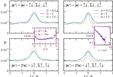
The explicit evaluation of the echo peak heights as given by Eq. (32) is carried out in Appendix C, yielding the general expressions (C9) and (C6) for the initial state and its spin- flipped counterpart, respectively. As shown in Fig. 4, these expressions are in excellent agreement with the results obtained from numerical simulations. For the particular case shown in Fig. 2(a), featuring an odd total number of particles, a full spin flip M = L and a real spin-orbit coupling ϕ = 0, the evaluation of Eq. (32) simplifies to

P

L,X^echo=id,T

(n, τ )

ϕ=0

=

2, τ = 0

1, τ 0 (33)

in agreement with the results of the numerical simulation. The highly nontrivial (and universal) dependence of P

_M,id^echo

with ϕ that follows from Eq. (32) is depicted in Fig. 4(a) for selected values M = 1, 4, 8 and compares remarkably well with the numerical simulations [56]. Such a good agreement is also seen in the detailed dependence of the echo peak on the number of flipped spins M for X = id [Fig. 4(b)] and X = T [Fig. 4(c)]

for ϕ = π/4.

(5)

FIG. 4. (a) Quantum-to-classical ratio P

M,id^echo

yielding the echo enhancement for the initial state | n according to Eq. (32) as a function of the SOC phase ϕ, for three different values of the number M of sites where spins are flipped. Panels (b) and (c), respectively, show the dependence of P

M,id^echo

and P

M,T^echo

on M at ϕ = π/4. Excellent agree- ment is found with the corresponding semiclassical predictions (C9) and (C6) for the echo enhancements on the initial state | n and its spin-flipped counterpart |Tn, respectively.

Finally, in order to estimate the τ dependence of the echo signals, we expand the actions in Eq. (10) to first order in time around τ = 0 and use the relation ∂R

γ

(t )/∂t =

− H

_mf

[ψ

^∗

(t ), ψ (t )] ≡ − E(n

, θ

) between the action and the conserved energy along classical trajectories, where we define θ

≡ (θ

₁_↑

, θ

₁_↓

, . . . , θ

_L_↑

, θ

_L_↓

) with θ

_lσ

= arg ψ

lσ

(t ) evaluated at the final time. Using standard ergodic methods, we obtain

P

M,X^echo

(n, τ ) P

M,X^echo

(n, 0) =

_2π

0

d

^2L

θ

(2π )

^2L

e

^iE(n,^θ^)τ/¯^h

²

(34) as shown in Appendix D. While this result suffers from an ambiguity in the definition of the mean-field Hamiltonian H

_mf

[46] (in contrast to the peak height calculation which is independent of the choice for H

_mf

), we can nevertheless infer from Eq. (34) some generic features of the MBSE peak width τ for the Hamiltonian (1). Using the fact that the interaction term within H

_mf

does not depend on the angle variables θ

lσ

allows us to infer that the energy difference E(n, θ) − E(n, θ

), which would arise in the exponent of the phase factor if we expand the modulus square expression within Eq. (34) into a double phase-space average integral, is independent of the spin-spin interaction strength U. As a consequence, the echo peak widths are insensitive to U . This intriguing result is indeed confirmed by the simulations presented in Fig. 5.

The dependence of the widths on the hopping parameters J and α can be estimated by realizing that the angle-dependent part of the classical energy E(n, θ) would most generally be constituted by a sum over terms that are proportional to κ

_{σ σ}

cos(θ

lσ

− θ

_l_+1,σ

) with κ

_{σ σ}

= − J and κ

_↑↓

= κ

_↓↑^∗

= αe

^iϕ

, where the involved proportionality factors depend on the occupancies n

lσ

in a manner that is specific to the choice of H

_mf

. The isolated integration over an angle variable within Eq. (34) would then yield a Bessel function J

₀

(γ τ ) with an argument proportional to τ , where the proportionality factor γ

FIG. 5. Echo peak profiles for |n

= |n (upper panels) and

| n

= | Tn (lower panels). P is plotted versus τ for various values of the interaction strength U at α = J /5 (left) and of the spin-orbit coupling α at U = J (right). The insets show the fitted peak widths τ (using a Lorentzian profile) for | n

= | n (“ + ” symbols) and

|n

= |n (“×” symbols) as a function of U at α = J /5 (left inset) and as a function of α at U = J (right inset). While the peak width is fairly independent of U within the wide parameter range where the mean-field dynamics is expected to be chaotic, it is found to scale with J and α as τ ∼ (J + α)

⁻¹

[ 1/max(J, α) if J α or J α], in agreement with the semiclassical prediction from Eq. (34).

would be given by an occupancy-dependent linear combination of J and α. We can therefore infer that the peak width roughly scales as τ ∼ 1/Max(J, α) where Max(J, α) denotes the maximum of the hopping J and the spin-orbit coupling α.

This prediction is also confirmed by the simulations as shown in Fig. 5.

IV. CONCLUSION

In conclusion, we predict the existence of a quantum

coherent effect that lifts the Hahn echo into the realm of

interacting quantum systems. The MBSE is a collective effect

observable at the level of many-body dynamics where in

few-fermion systems, and due to quantum interference, the

system echoes either its initial or its spin-flipped state after

a sudden flip of the spins. Using a semiclassical approach

based on interfering paths in Fock space, we show the relation

between the many-body spin echo and antiunitary symme-

tries. We predict that its signal has a universal dependence

on few microscopic parameters if the classical mean-field

dynamics displays chaotic behavior. This nonperturbative,

chaotic regime where interactions, hopping, and spin-orbit

coupling are of similar strength is accessible in experimental

realizations using fermionic cold atoms, coupled quantum dots,

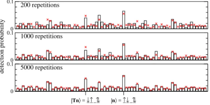
or small molecules. As shown in Fig. 6, simulations of possible

experiments indicate that a system of four particles in four sites

should already be sufficient to observe the MBSE after a few

thousand runs. This can be routinely done with ultracold atoms

in optical lattices using state-of-the-art single-site detection

techniques [57], and is within reach in setups using quantum

dot arrays [24,25,28,38,39].

(6)

FIG. 6. Numerical simulation of the post-selection process for a Fermi-Hubbard chain with L = 4 sites and half-filling (with the same parameters as in Fig. 2). For each disorder realization a Fock state is randomly chosen according to the computed final-state probabilities (whose disorder average is marked by red crosses). After some 1000 repetitions of this numerical experiment, the echo effect becomes clearly visible.

Our analytical results agree perfectly with extensive nu- merical simulations. They show that the many-body spin echo is a defining signature of many-body coherence in systems modeled by Fermi-Hubbard Hamiltonians. This establishes the long-sought connection between chaotic mean-field dy- namics and universal coherent effects for fermionic fields. It suggests that semiclassical techniques to calculate echo-related observables, such as out-of-time ordered correlators in bosonic many-body systems [58], can be extended from the bosonic to the fermionic domain.

ACKNOWLEDGMENTS

We thank H. Baranger for illuminating discussions. Support from DFG through Projects No. C6 of SFB 689 and No. A07 of CRC 1277 is gratefully acknowledged.

APPENDIX A: CLASSICAL TRANSITION PROBABILITY The diagonal approximation yields the classical probabil- ity (12) to detect the final occupancies n

, which is determined by the classical transition probability p

_cl

(m, n; t ) from the initial occupancies n to the final ones m at time t. Assuming a fully ergodic system, this classical probability is, on average, expected to be independent of time as well as of the initial and final occupancies. We therefore propose

p

_cl

(m, n; t ) = 1/ N , (A1) where N is the number of possible final occupancies m satisfying the conservation of the total particle number

L

l=1

(m

l↑

+ m

l↓

) = N, (A2) as well as the Pauli principle requiring that two particles with the same spin must not be located on the same site, i.e., m

_lσ

∈ { 0, 1 } for all 0 l L and σ = ↑ , ↓ [59]. In other words, N is the dimension of the Hilbert space for N fermionic spin-

¹₂

particles on L sites and can be determined by counting the number of possibilities to populate N out of 2L single-particle states with a fermion (the factor 2 accounts for the two possible

choices for the spin). This standard problem in statistics has the well-known solution

N = 2L

N

. (A3)

The classical probability (12) is then evaluated as P

_cl

(n

, n; τ ) =

m

1 N

²

= 1

N , (A4) where we assume that the averages over the two propagation steps in the classical limit can be performed independently.

A more formal derivation of Eq. (A1) can be obtained through realizing that we can express the semiclassical ampli- tude prefactor | A

γ

|

²

associated with a trajectory γ that evolves from n to m within time t as

| A

γ

|

²

= 1 (2π )

^2L

det

∂θ

_lσ^(γ⁾

∂m

lσ

(m, n, t )

2L×2L

, (A5) where θ

_lσ^(γ⁾

= arg ψ

_lσ^(γ⁾

(0) is the trajectory’s initial angle vari- able on the site l with the spin σ . A standard sum rule argument then yields

γ

| A

_γ

|

²

=

_2π

0

d

^2L

θ

(2π )

^2L

δ[m ˜ − I(n, θ , t)] (A6) with θ ≡ (θ

1↑

, θ

₁_↓

, . . . , θ

_L_↑

, θ

_L_↓

), where we define by I(n, θ , t ) the final action variables that result from propagating the initial field ψ ≡ (ψ

_1↑

, . . . , ψ

L↓

) with ψ

lσ

= n

^1/2_lσ

exp(iθ

lσ

) over time t. Owing to the conservation of the total action [

lσ

I

lσ

(n, θ , t ) = N for all t ], the multidimensional delta function appearing in Eq. (A6) has to be defined such that one of the involved dimensions is not accounted for, e.g.,

δ(m ˜ − I) ≡ δ(m

L↑

− I

L↑

)

L

−1

l=1

σ=↑,↓

δ (m

lσ

− I

lσ

). (A7) Defining correspondingly

m

≡

∞ m_1↑=−∞

∞ m_1↓=−∞

. . .

∞ m_L↑=−∞

, (A8)

we obtain through the application of Poisson’s summation formula

m

γ

| A

γ

|

²

=

∞ k_1↑=−∞

∞ k_1↓=−∞

. . .

∞ k_L↑=−∞

_2π

0

d

^2L

θ (2π )

^2L

× exp

2πi

l,σ

k

_lσ

I

_lσ

(n, θ , t)

. (A9) Owing to the classical Hamiltonian dynamics generated by H

_mf

, which grants the conservation of the total action and ought to inhibit the occurrence of individual action variables I

lσ

(n, θ , t) acquiring integer values that exceed 1, this latter expression (A9) is actually identical to

m

γ

| A

_γ

|

²

where here the sum over m is restricted to binary occupancies m

_lσ

∈ {0, 1} that satisfy Eq. (A2).

Subjecting Eq. (A9) to a disorder average gives, due to

the presence of the rapidly oscillating phase factors, rise to

cancelations of all terms in the multiple sum except for the

(7)

k

_1↑

= k

_1↓

= · · · = k

_L_↑

= 0 term for which the multidimen- sional integral on the right-hand side of Eq. (A9) yields unity.

Noting furthermore that we can identify p

_cl

(m, n; t ) with the disorder average of

γ

| A

γ

|

²

and that in a perfectly ergodic system p

_cl

ought to be independent of m provided Eq. (A2) is fulfilled, we can rewrite the disorder average of Eq. (A9) as N p

_cl

(m, n; t ) = 1. This confirms the validity of Eq. (A1).

Owing to Eq. (A6), it actually amounts to stating that the disorder average of ˜ δ[m − I(n, θ , t)] equals 1/ N .

APPENDIX B: TIME-INDEPENDENT BACKGROUND The time-independent increase or decrease compared to the classical probability originates from those terms in the sum over intermediate occupancies m that satisfy F

^(M)

m = m, i.e., the corresponding Fock state remains invariant under the spin-flip operation. Furthermore, for an arbitrary time mismatch τ , a pairing of the types (25) and (26) is possible only if the trajectories γ

₁

and γ

₂

join smoothly, i.e., if γ

₂

is the continuation of γ

₁

, as shown in Fig. 3(c). These contributions yield remnants of the coherent backscattering and forward scattering as addressed in Ref. [46]. The corresponding action differences are evaluated from Eqs. (27) and (28) as

^γγ³1^γγ⁴2

π

L

l=1

(n

l↓

− n

_l_↑

) for the pairing (25) and

^γγ³₁^γγ⁴₂

0 for the pairing (26), and do not depend on the intermediate occu- pancies m. Thus, assuming fully ergodic classical transition probabilities given by Eq. (A1), the echo enhancement for τ 0 is obtained by counting the number N

_e⁽⁰⁾

of possible intermediate occupancies m that satisfy F

^(M)

m = m while respecting the relation (A2) that expresses the conservation of the total number of particles. This condition implies m

l↑

= m

l↓

for 1 l M, i.e., each one of the first M sites of the lattice is either empty or doubly occupied.

In order to determine the number N

_e⁽⁰⁾

of possible inter- mediate occupancies, let us first consider a fixed choice for the occupancies m

l↑

= m

l↓

∈ { 0, 1 } on the first M sites of the lattice, with each of those sites being either empty or double occupied. If k is the number of double-occupied sites among this set, we have

_2(L₋_M₎

N−2k

possibilities to distribute the remaining N − 2k spin-

¹₂

particles within the remaining L − M sites of the lattice. Taking furthermore into account that there are

_M

k

such possibilities to have k out of M sites being doubly occupied with the other M − k sites being empty, we finally obtain

N

_e⁽⁰⁾

=

min(M,

N/2)

k=0

M k

2(L − M) N − 2k

, (B1) with x denoting the integer part of x. This consideration yields for τ 0

P

M,X^echo

(n; τ ) = P ¯ (Xn, n; τ ) P ¯

_cl

(Xn, n; τ )

τ

=

0

(−1)

^{N δ}^X

N

_e⁽⁰⁾

N , (B2) for X = id or T, defining δ

_id

= 0 and δ

T

= 1.

APPENDIX C: PEAK HEIGHT OF THE ECHO ENHANCEMENT

We now focus on the derivation of the echo enhancement at vanishingly small mismatch times τ = 0 with respect to

the time-independent background. The latter is, as was dis- cussed in the previous section, constituted by terms satisfying F

^(M⁾

m = m for the intermediate occupancies, which are valid for all times τ including τ = 0. Strictly speaking, those terms with F

^(M⁾

m = m should therefore be excluded from the sums for the contributions from the pairings (25) and (26) at the echo time τ = 0. For the sake of simplicity, we nevertheless include them in the subsequent calculations. The time-independent background (B2) needs therefore to be subtracted from the final expressions (C6) and (C9) in order to properly determine the peak height.

1. Echo on the spin-flipped counterpart of the initial state The quantum contribution for the detection probability of the Fock state with the occupancies n

= Tn, with T = F

^(L)

the full spin-flip matrix, is determined by the pairing (25).

The resulting action differences (11) are evaluated by means of Eq. (27). Using (F

^(M⁾

m)

l↑

= m

l↓

for 1 l M whereas (F

^(M⁾

m)

l↑

= m

l↑

if l > M , we obtain

^Tγ₁^γγ²₂^T^γ¹

= π

_L

l=1

(n

l↓

− n

l↑

) +

M

l=1

(m

l↑

− m

l↓

)

= 2π

_L

l=1

n

l↓

−

M

l=1

m

l↓

− π N

L−M

(C1) taking into account again Eq. (A2), where we define by

N

L−M

=

L

l=M+1

(m

l↑

+ m

l↓

) (C2) the number of particles that are not affected by the spin flip at the time t

_F

. This yields

exp

i

^Tγ₁^γγ²₂^T^γ¹

= (−1)

^N^L−M

. (C3) We therefore infer from Eq. (10) that the combination of the trajectories γ

₁

before and γ

₂

after the spin flip contributes with a positive or negative sign to the average echo enhancement depending on whether N

L−M

is even or odd.

Thus, the peak height at the echo point τ = 0 for the spin-reversed counterpart of the initial state is obtained by counting the numbers N

e

and N

o

of possibilities to place an even or odd number N

_L₋_M

of fermionic spin-

¹₂

particles, respectively, within L − M sites of the lattice. To this end, we need to determine the number of possibilities to distribute N

L−M

fermions onto 2(L − M) single-particle states, which is to be multiplied by the number of possibilities to distribute the remaining N − N

_L₋_M

fermions onto the remaining 2M states of the underlying one-body system. Substituting N

L−M

= 2k or N

L−M

= 2k + 1 with integer k and then summing over all possible values of k yields

N

e

=

N/2 k=0

2(L − M) 2k

2M N − 2k

, (C4)

N

o

=

N/2 k=0

2(L − M) 2k + 1

2M N − 2k − 1

, (C5)

(8)

with x denoting the integer part of x. With those two num- bers, the echo enhancement for X = T at τ = 0 is evaluated as

P

M,T^echo

(n; τ = 0) = 1 + N

e

− N

o

N . (C6) 2. Echo on the initial state

The pairing (26) requires n

= n and thus gives a contribu- tion for the probability to detect the initial state. The resulting action differences (27) are evaluated by means of Eq. (28).

Using (F

^(M⁾

m)

l↑

= m

l↓

and (F

^(M)

m )

l↓

= m

l↑

for 1 l M whereas (F

^(M)

m)

lσ

= m

lσ

for σ = ↑ , ↓ if l > L, we obtain

^{T S}^γ1γ^ϕ₂^γ²^{T S}^ϕ^γ¹

= 2ϕ (k

_↓

− k

_↑

), (C7) where we define by

k

σ

=

M

l=1

m

lσ

(C8)

the total number of particles whose spin is flipped from σ to the opposite spin at the time t

F

. Thus, the average detection probability for the initial state at the echo time τ = 0 is given by

P

_M,id^echo

(n; τ = 0) = 1 + f (N, M; ϕ )

N (C9)

with

f (N, M ; ϕ) =

N k_↑=0

N

−k_↑

k_↓=0

N

k_↑,k_↓

exp

2iϕ(k

_↓

− k

_↑

) . (C10) Each term in this double sum is weighted by the number

N

k_↑,k_↓

=

m

δ

M l=1

m_l↑,k_↑

δ

M l=1

m_l↓,k_↓

(C11) of possible occupancies that feature k

_↑

spin-up and k

_↓

spin- down particles in the flipped sites. This number is given by the product of the numbers of possibilities to distribute k

σ

fermionic particles with spin σ to M sites for σ = ↑ and σ = ↓, which is to be multiplied with the number of possibilities to distribute the remaining N − k

_↑

− k

_↓

particles to the remaining L − M sites. This yields

N

k_↑,k_↓

= M

k

_↑

M

k

_↓

2(L − M) N − k

_↑

− k

_↓

. (C12)

APPENDIX D: ECHO PEAKS AT FINITE MISMATCH TIME In contrast to the peak heights, which are entirely deter- mined by the symmetries of the system and therefore do not depend on the details of the mean-field Hamiltonian H

_mf

, the calculation of the peak widths is sensitive to properties of the specifically chosen H

_mf

. Some qualitative and quantitative features of the peak widths can nevertheless be obtained even without the precise knowledge of the classical Hamiltonian provided the interaction term of the latter can be exclusively expressed in terms of the spin-dependent onsite populations I

lσ

= | ψ

lσ

|

²

and does not depend on the associated angle variables θ

lσ

= arg(ψ

lσ

). As is seen in Eq. (1), this is indeed the case for the many-body system under consideration.

Let us first note that τ -dependent contributions necessarily arise from the pairings (25) and (26) that involve a time-reversal operation. They are provided by correlated trajectory pairs in which one of the partners is defined for the evolution time t

F

while the other one evolves until t

F

+ τ . This mismatch in the evolution times gives rise to additional contributions to the combined action differences (11) as compared to Eqs. (C1) or (C7).

To be specific, let us consider such a correlated trajectory pair (γ , γ

) in which γ evolves from the initial occupancies n to some intermediate occupancies m within the time t

F

while γ

evolves from F

^(M⁾

m

to the final occupancies n

within the time t

F

+ τ . For not too large mismatch times, the action associated with the latter trajectory can be approximated through a Taylor expansion

R

_γ

(t

F

+ τ ) R

_γ

(t

F

) + τ ∂

∂t

R

_γ

(t

)

t=t_F

+ O (τ

²

) (D1) about the evolution time t

_F

, where we formally define R

_γ

(t ) ≡ R

γ(t)

with γ

(t

) representing the continuous family of tra- jectories that evolve from F

^(M⁾

m

to n

within the time t

and yield γ

(t

) = γ

for t

= t

F

+ τ . Now, we use the well-known property

∂

∂t

R

_γ

(t

) = − E

_γ

(t

) (D2) of the classical action, where E

γ

(t

) = H

_mf

(ψ

^γ^∗

, ψ

^γ

) ≡ E

γ(t)

is the (conserved) classical energy of the trajectory γ

(t

), defined as a function of the propagation time t

. As (γ , γ

) is supposed to be a correlated trajectory pair, E

_γ

(t

F

) is identical to the energy E

γ

≡ E

γ

(t

F

) of the partner trajectory γ . The action difference associated with this pair is then approx- imately evaluated as R

γ

− R

γ

R

γ(tF)

− R

γ

− E

γ

τ where the difference R

_γ(tF)

− R

_γ

is provided by the expression (27) or (28), depending on the final state under consideration.

In practice, we are dealing in Eq. (10) with the correlated trajectory pairs (γ , γ

) = (γ

1

, γ

₄

) and (γ

3

, γ

₂

). The combined action differences (11) are then evaluated as

^γγ³₁^γγ⁴₂

=

^Xγ₁^γγ²₂^X^γ¹

+ τ

¯

h [E

γ1(tF)

− E

_γ₂_(t_F₎

] + O(τ

²

) (D3) in linear order in the mismatch time, with X = T for n

= Tn and X = T S

ϕ

for n

= n. As was shown above, the respective expressions (C1) and (C7) for

^X^γ1^γγ²₂^X^γ¹

depend only on the intermediate occupancies m

lσ

and not on the precise choice for the trajectories that link them to the initial and final states, i.e., we can redefine

^Xγ₁^γγ²₂^X^γ¹

≡

X

(m) with X = T or id, respectively. This allows us to carry out the summations over γ

₁

and γ

₂

separately by means of standard sum rules in close analogy with Eq. (A6), namely, according to

γ₁

| A

γ₁

|

²

e

^{iτ E}^γ¹^/¯^h

=

_2π

0

d

^2L

θ

(2π )

^2L

δ[m ˜ − I(n, θ , t

F

)]

× exp [iτ E(n, θ )/¯ h] (D4)

(and similarly for γ

₂

, with opposite sign of τ ), where ˜ δ

is defined through Eq. (A7) and where we introduce by

E(n, θ ) = H

_mf

(ψ

^∗

, ψ ) with ψ ≡ (ψ

1↑

, . . . , ψ

L↓

) and ψ

lσ

=

n

^1/2_lσ

exp(iθ

lσ

) the total energy associated with the action-angle

(9)

variables (n, θ). This yields P (n

, n; τ )

m

e

ⁱ^X^(m)

_2π

0

d

^2L

θ (2π )

^2L

_2π

0

d

^2L

θ

(2π )

^2L

× e

^iτ[E(n,^θ⁾⁻^E(n^,^θ^)]/¯^h

δ[m ˜ − I(n, θ , t

_F

)]

× δ[F ˜

^(M⁾

(m ) − I(n

, θ

, − t

F

)] (D5) for the semiclassical transition probability from n to n

.

Following the line of reasoning that we carried out above in the discussion of the diagonal approximation, we permit ourselves to replace each one of the multidimensional delta

functions appearing in Eq. (D5) by the constant 1/ N in the presence of a disorder average, assuming again perfect classical ergodicity. This approximation finally yields Eq. (34).

It essentially relies on the assumption that the relative weight of intermediate occupancies satisfying F

^(M)

m = m is rather small for sufficiently large M. Indeed, for those intermediate occupancies the trajectories γ

₁

and γ

₂

would join smoothly, and hence there would be a systematic correlation between θ and θ

such that E(n, θ) = E(n

, θ

). We also assume here that the an- gle average over exp[iτ E(n

, θ

)/¯ h] can be straightforwardly transformed into an angle average over exp[iτ E(n, θ)/ h] ¯ through an appropriate change of variables θ

→ θ if n

= Tn.

[1] E. L. Hahn, Phys. Rev. 80, 580 (1950).

[2] V. N. Prigodin, B. L. Altshuler, K. B. Efetov, and S. Iida, Phys.

Rev. Lett. 72, 546 (1994).

[3] A. Peres, Phys. Rev. A 30, 1610 (1984).

[4] J. H. Malmberg, C. B. Wharton, R. W. Gould, and T. M. O’Neil, Phys. Rev. Lett. 20, 95 (1968).

[5] R. Pierrat, C. Vandenbem, M. Fink, and R. Carminati, Phys. Rev.

A 87, 041801 (2013).

[6] J. R. Klauder and P. W. Anderson, Phys. Rev. 125, 912 (1962).

[7] R. A. Jalabert and H. M. Pastawski, Phys. Rev. Lett. 86, 2490 (2001).

[8] E. Abe, K. M. Itoh, J. Isoya, and S. Yamasaki, Phys. Rev. B 70, 033204 (2004).

[9] W. M. Witzel, R. de Sousa, and S. Das Sarma, Phys. Rev. B 72, 161306 (2005).

[10] T. Micklitz, C. A. Müller, and A. Altland, Phys. Rev. B 91, 064203 (2015).

[11] K. Müller, J. Richard, V. V. Volchkov, V. Denechaud, P. Bouyer, A. Aspect, and V. Josse, Phys. Rev. Lett. 114, 205301 (2015).

[12] X. X. Yi, H. Wang, and W. Wang, Eur. Phys. J. D 45, 355 (2007).

[13] W.-L. Ma, G. Wolfowicz, N. Zhao, S.-S. Li, J. J. L. Morton, and R.-B. Liu, Nat. Commun. 5, 4822 (2014).

[14] L. Luan, M. S. Grinolds, S. Hong, P. Maletinsky, R. L.

Walsworth, and A. Yacoby, Sci. Rep. 5, 8119 (2015).

[15] C. Solaro, A. Bonnin, F. Combes, M. Lopez, X. Alauze, J.-N.

Fuchs, F. Piéchon, and F. Pereira Dos Santos, Phys. Rev. Lett.

117, 163003 (2016).

[16] M. Knap, A. Kantian, T. Giamarchi, I. Bloch, M. D. Lukin, and E. Demler, Phys. Rev. Lett. 111, 147205 (2013).

[17] M. Serbyn, M. Knap, S. Gopalakrishnan, Z. Papi´c, N. Y. Yao, C. R. Laumann, D. A. Abanin, M. D. Lukin, and E. A. Demler, Phys. Rev. Lett. 113, 147204 (2014).