E SSAYSIN E NERGY E CONOMICS

E ^{SSAYS IN} E ^NERGY E ^CONOMICS

Inauguraldissertation zur

Erlangung des Doktorgrades der

Wirtschafts- und Sozialwissenschaftlichen Fakultät der

Universität zu Köln 2017 vorgelegt

von

Diplom-Volkswirt Simon Paulus aus

Lennestadt

Referent Prof. Van Anh Vuong, Ph.D.

Korreferent Prof. Dr. Marc-Oliver Bettzüge

Tag der Promotion 12.12.2017

Acknowledgements

For supervising my dissertation, I firstly would like to thank my supervisor Prof. Van Anh Vuong, Ph.D. for her support. She provided fruitful and constructive comments helping me to improve each of my articles. I also would like to thank Prof. Dr. Marc- Oliver Bettzüge for offering me the chance to theoretically learn and grow in the academic field of energy-economic research and his helpful advice and suggestions on the articles that have been embedded in this thesis.

Furthermore, I am grateful for the inspiring collaboration with Dr. habil. Christian Growitsch, Dr. Andreas Knaut, Martin Paschmann and Prof. Dr. Heike Wetzel on the joint research articles that individually but also taken together widened my horizon.

In addition, I am thankful to my colleagues at ewi Energy Research & Scenarios for the many fruitful discussions and ideas in the broad field of energy markets. In particular, my thanks go to Joachim Bertsch, Broghan Helgeson, Jakob Peter and Johannes Wagner and finally yet importantly to Zorica Marijanovi´c, Maria Novikova and Lena Pickert who provided excellent research assistance.

Finally, I would like to thank my family.

Simon Paulus Cologne, October 2017

Contents

Acknowledgements

List of Figures

List of Tables

1 Introduction

1.1 Introducing the Essays . . . . 2

1.2 Future Research and Possible Improvements to Methodologies . . . . 4

2 When Are Consumers Responding to Electricity Prices? An Hourly Pattern of Demand Elasticity

2.1 Introduction . . . . 7

2.2 Measuring Market Demand Reactions Based on Wholesale Prices . . . 10

2.2.1 The Retail Market for Electricity . . . . 10

2.2.2 The Wholesale Market for Electricity . . . . 11

2.2.3 The Interaction of Wholesale and Retail Markets . . . . 13

2.3 Empirical Framework . . . . 15

2.3.1 Data . . . . 15

2.3.2 Econometric Approach . . . . 18

2.4 Empirical Application . . . . 20

2.5 Conclusion . . . . 23

2.6 Appendix . . . . 25

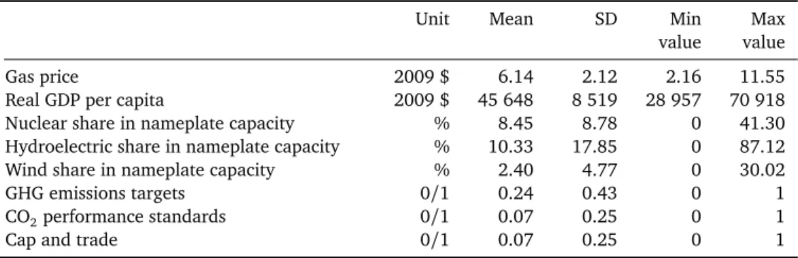
3 Competition and Regulation as a Means of Reducing CO

-Emissions - Experience from U.S. Fossil Fuel Power Plants

3.1 Introduction . . . . 27

3.2 U.S. electricity generation from fossil fuels 2000 - 2013 . . . . 29

3.3 Empirical approach . . . . 32

3.3.1 Benchmarking model . . . . 32

3.3.2 Benchmarking data . . . . 37

3.3.3 Second-stage regression . . . . 38

3.4 Results . . . . 42

3.4.1 Benchmarking results . . . . 42

3.4.2 Second-stage regression results . . . . 47

3.5 Conclusions . . . . 50

4 The Impact of Advanced Metering Infrastructure on Residential Electricity Consumption - Evidence from California

4.1 Introduction . . . . 53

4.2 Literature Background . . . . 55

4.3 Identification Strategy . . . . 57

4.4 The Californian Case . . . . 59

4.5 Data . . . . 63

4.5.1 Dependent Variable: Residential Electricity Consumption . . . 63

4.5.2 Explanatory Variables . . . . 65

4.6 Empirical Analysis . . . . 67

4.6.1 Derivation of the Control Group Using Synthetic Controls . . . 67

4.6.2 Difference-in-Differences Estimation Results . . . . 71

4.7 Conclusion . . . . 77

4.8 Appendix . . . . 79

5 Electricity Reduction in the Residential Sector - The Example of the Californian Energy Crisis

5.1 Introduction . . . . 85

5.2 Literature . . . . 87

5.3 The Energy Crisis and its containment through conservation programs 90 5.4 Data . . . . 92

5.4.1 Dependent Variable: Residential electricity consumption . . . 93

5.4.2 Explanatory Variables . . . . 93

5.5 Empirical Application . . . . 96

5.5.1 Synthetic control group derivation and results . . . . 96

5.5.2 Two-stage least-squared treatment regression and results . . . 99

5.6 Conclusion . . . 104

5.7 Appendix . . . 107

Bibliography

Curriculum Vitae

viii

List of Figures

2.1 Electricity price formation on the wholesale market . . . . 12 2.2 Supply and demand curves for one exemplary hour . . . . 14 2.3 Hourly data for load, electricity price, wind and solar generation for

2015 . . . . 16 2.4 Correlations with load and prices in 2015 . . . . 19 2.5 Hourly dummies and price elasticity of electricity demand in 2015 . . 21 2.6 Prices for coal, gas and co2 certificates from January to December 2015 25 3.1 Cost of fossil fuel receipts at electricity generating plants in USD per

million Btu . . . . 30 3.2 Shares of total U.S. net electricity generation from fossil fuels in % . 31 3.3 Global Malmquist CO

emission performance index (GMCPI) . . . . . 34 3.4 Cumulative GMCPI trends for the top and bottom performers for the

period 2000-2013 . . . . 48 4.1 Smart-metering legislation across the US states (Energy Information

Administration 2011) . . . . 58 4.2 Investor-Owned Utilities (IOUs) and the respective share of Califor-

nian customer accounts (2015, Dec.) . . . . 60 4.3 Share of Californian (three major IOUs) households with AMI (smart

meters) over time . . . . 62 4.4 Candidate states with low AMI penetration . . . . 70 4.5 Descriptive comparison and differences between the development of

residential electricity consumption in California and ‘Synthetic Cali- fornia’ . . . . 72 4.6 Simplified illustration of Advanced Meter Infrastructure (AMI) and its

informational feedback . . . . 79

4.7 Development of energy-efficiency savings in California over time . . . 80

4.8 Simplified schedules for tier and time-of-use in the residential sector 84

5.1 Californian residential electricity consumption and conservation pro- grams . . . . 92 5.2 Descriptive Comparison for the ’Synthetic Control Group’-State (SECC)

and California . . . . 99 5.3 Sample bill including ’20

20’ rebate for residential customers.

Source:

Southern California Edison, 2017

. . . 107 5.4 Un- or scheduled capacity revisions by IOUs in MW.

Source: Blum-

stein et al., 2002

. . . 107 5.5 Synthetic Control Results - Difference Plot . . . 109 5.6 Residential consumption in pre-selected states over 48-month period 113

x

List of Tables

2.1 Literature review of estimated short-run elasticity . . . . 9

2.2 Descriptive statistics (for weekdays, without public holidays and Christ- mas time) . . . . 15

2.3 Regression results . . . . 22

3.1 Descriptive statistics: state-level data 2000 to 2013 . . . . 38

3.2 Determinants of CO

emission performance: summary statistics . . . 40

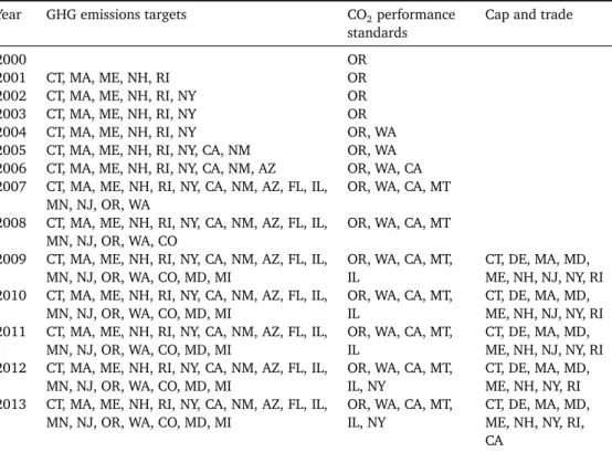
3.3 State-specific regulatory policies . . . . 41

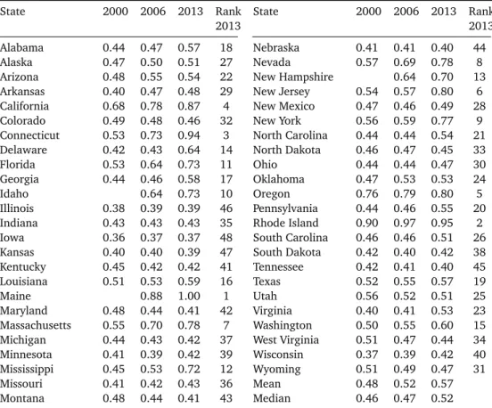
3.4 CO

emission efficiency scores per state . . . . 43

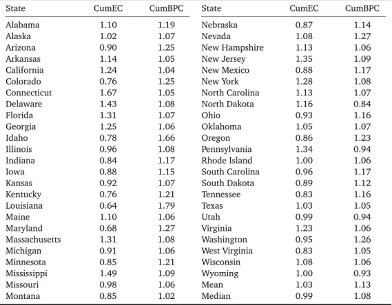
3.5 Cumulative GMCPI per state over the period 2000-2013 (2000

1) . 45 3.6 Cumulative GMCPI decomposition per state over the period 2000- 2013 (2000

1) . . . . 46

3.7 Determinants of CO

emission performance: estimation results . . . . 49

4.1 Energy efficiency savings data . . . . 65

4.2 List of variables and references . . . . 68

4.3 Descriptive statistics . . . . 69

4.4 IV Estimates for DiD estimation . . . . 75

4.5 Descriptive statistics: Differences in levels (California minus Synthetic California) . . . . 80

4.6 Weights of the exogenous variables . . . . 81

4.7 IV Estimates for DiD estimation when controlling for yearly time dum- mies . . . . 83

5.1 List of variables and references . . . . 95

5.2 Determinants of monthly residential electricity consumption: IV esti- mation results . . . 103

5.3 Descriptive Statistics . . . 108

5.4 Weights of the exogenous variables . . . 108

5.5 IV Estimates when controlling for pre- and post crisis treatment time

dummies . . . 115

1 Introduction

Energy economic research contributes to a better understanding of energy markets, such as resource and electricity markets. Within this broad field, research on mar- kets, policy interventions and environmental issues is, among others, conducted.

One unique characteristic of energy markets, serving as ‘common ground’ for aca- demic studies in the field of energy economics, is the condition of a reliable power supply that satisfies power consumption over time and even more importantly in real time. Given that supply and demand levels could change (rapidly) on a tem- poral scale, based on for instance forced generation unit, transmission line outages, sudden load changes or regulations, this seemingly unremarkable condition has far- reaching implications for generators, consumers and policy makers alike. Whereas both, the demand and supply side can individually contribute to a secure system, policy makers may be willing to set the right framework for energy markets and correct market failures or even implement policy instruments for a desired outcome.

In this thesis, the following four essays on energy economics, covering the listed topics, are presented. Each chapter is based on a single article to which the authors contributed equally:

Chapter 2: When are Consumers Responding to Electricity Prices? An Hourly Pattern of Demand Elasticity (based on Knaut & Paulus (2016))

Chapter 3: Competition and Regulation as a Means of Reducing CO

-Emissions - Experience from U.S. Fossil Fuel Power Plants (based on Growitsch et al. (2017)) Chapter 4: The Impact of Advanced Metering Infrastructure on Residential Electric- ity Consumption - Evidence from California (based on Paschmann & Paulus (2017)) Chapter 5: Electricity Reduction in the Residential Sector - The Example of the Cal- ifornian Energy Crisis (based on Paulus (2017))

The four essays are stand-alone and may be read in any order; however, with

the analysis of the demand side in Chapter 2, I intend to shed some light on the

commonly assumed inelastic demand assumption in electricity markets by study-

ing the German market. Chapter 3, 4 and 5 study policy interventions affecting

both, the generation and demand side in electricity markets. Whereas Chapter 3

1 Introduction

addresses policy intervention directed towards environmental protection, Chapter 4 and 5 rather investigate the impact on residential demand reduction through policy interventions specifically targeting a change in electricity usage.

The presented methodologies to tackle the issues discussed and the topic selection itself are guided by the author’s interest. The following introduction provides a brief summary of the four essays, including the research question and a brief discussion of the results. Furthermore, the author sets out how each of the four essays adds to existing literature and serve for a better understanding of the investigated top- ics. The introduction concludes with possible extensions for future research, critical reflections and some improvements to methodologies for the essays.

1.1 Introducing the Essays

Chapter 2 focuses on the demand elasticity in the German wholesale market by ap- plying a two stage least-squared estimation technique. Complementary to already conducted research, the estimated demand elasticity is not sub-market specific. The estimation is based on hourly time intervals. It is motivated by the thought that utility resulting from electricity consumption for all end consumers differs in every hour. Thus, the higher temporal resolution reveals hourly patterns for demand elas- ticities ranging from -0.02 to -0.13 for the analyzed market area. The article adds to attempts for measuring demand elasticities of higher temporal order in electricity market by building on some initial thoughts of Bönte et al. (2015). However, an analysis for Germany is so far lacking in the literature. Our analysis makes use of the stochastic character of renewable generation that primarily affects the supply side but not the demand side thereby serving as a suitable instrument in order to solve simultaneity issues occurring in electricity markets. The found hourly elasticity results for the German market may be used for further academic studies attempting to model electricity markets with simulation methods where commonly demand de- velopments for sectors are a prior defined as perfectly ‘inelastic’, a restriction that from the author’s point of view is implicitly questioned.

Chapter 3 investigates the influences of regulation and gas prices on the emission levels of fossil power plants for all states in the U.S. Research has been motivated by the rising influence of shale gas in the past decade influencing gas prices and con- sumption. It furthermore investigates the switch from a heavily coal-based genera- tion portfolio to a less carbon-intense gas-fired generation portfolio over a thirteen years period by taking gas price effects and a tightened CO

-regulation for emis-

2

1.1 Introducing the Essays

sion in the generation portfolio into account. The essay is based on Growitsch et al.

(2017) and uses nonparametric benchmarking techniques to first identify best prac- tice states between 2000 and 2013. Example states and their generation portfolios are used to back up results obtained by the approach and provide an intuitive under- standing for some states, where initial interpretation of benchmarking results may not be straightforward (i.e. for North Dakota). Secondly, a regression on the CO

emission performance over time is conducted by controlling among others for gas prices and all CO

-related regulation, occurring in the form of emission standards and cap and trade systems. The empirical analysis presented in Chapter 3 adds to the literature on benchmarking within the power generation field, where good and bad outputs need to be simultaneously modeled. We make use of the standard as- sumptions of Färe & Primont (1995) and extend the standard model of Shephard (1953) by using an input distance function allowing for a multi-input and output simulation that is indispensable when analyzing emissions of fossil power genera- tion. Besides best practice states, our results show lower gas prices and stringent CO

regulations are suitable means to reduce CO

emissions.

Chapter 4 analyzes the policy-induced Advanced Metering Infrastructure deploy- ment in California and the related impact of additional information on residential electricity consumption. Contrary to the other chapters, Chapter 4 is positioned in the literature on behavioral economics linking informational feedback, the nature of consumers being rationally bounded with residential electricity consumption (as for instance also done by Allcott & Rogers (2014)). A rather systemic perspective is framing this chapter by analyzing the respective impact of Advanced Metering In- frastructure deployment on electricity savings. With the help of synthetic control techniques (Abadie et al., 2010), the obstacle of not having a direct control group within a large-scale framework is overcome. A Difference-in-Differences estimation accounts for causality and persistency matters over a 13-year period. As such, the chosen approach differs with respect to test pilots analyzing shorter time spans and the fact that a subsample of the population may cause severe estimation bias. The results show a significant negative impact of Advanced Metering Infrastructure on monthly residential electricity consumption that ranges from 6.1% to 6.4% over the respective period. Additionally, an impact of Advanced Metering Infrastructure on residential electricity consumption only occurs in non-heating periods and does not fade out over the analyzed time period.

Chapter 5 investigates supply shortages in the Californian electricity market and

the role of policy measures to contain the Energy Crisis. The contribution of this

1 Introduction

paper lies not only in the assessment of policy measures and electricity price effects to curb residential electricity consumption, it furthermore reveals that consumption in the Californian residential sector may be reduced by up to 12% triggered partly by an adjustment within respect to secondary energy use in the residential sector. As my results show, this ‘reduction potential’ or ‘residential comfort buffer’ is more likely to be leveraged in summer periods which I relate to comfort issues that consumers are not willing to ’sacrifice’ on in winter periods. Chapter 5 adds to the discussing of electricity price impacts in residential electricity markets (Albadi & El-Saadany, 2008) and the effectiveness of short term policy measures targeting residential elec- tricity reduction rather than technical replacements of household appliances that commonly cover longer time periods. It is thus positioned in the context of policy measures not related to changing technical household appliances. Methodologically, Chapter 5 makes uses of a synthetic control group derivation. A nationwide analysis for the impact of conservation programs, in particular the ’20

20’ rebate program and the mass media campaign, emerging from the Californian Energy Crisis has not been conducted so far. The mutual impact of conservation impacts is estimated via a treatment regression.

1.2 Future Research and Possible Improvements to Methodologies

Expect for Chapter 4 and 5 mutually sharing the application of a synthetic con- trol group derivation, all four chapters address different research questions, each of which requires a different methodology. Chapter 3 presents a non-parametric benchmarking approach to model emission improvements over time, followed by an applied econometric method. Even though the baseline model is extended by the features of multiple inputs and outputs, reflecting that emissions cannot be reduced without reducing electricity generation, some researchers tend to rather follow the material balance constraint programing (i.e. Førsund (2008)) essentially imposing the condition that residuals cannot be used when jointly modeling input and output on a multi-dimensional level. The critique applied to previous literature may there- fore also apply to the analysis presented here. In addition, the model may fail to in- corporate important features of the industry on a micro level. Firm specific data may thus grasps the fundamental industry structure of the fossil generation with more detail. However, it may also be noted that the aggregated data used by the authors stems from a detailed data survey conducted by the Energy Information Adminis-

4

1.2 Future Research and Possible Improvements to Methodologies

tration agency in the U.S. (i.e. EIA form-860) that builds upon data collection on the power plant unit level. Although numerous estimation specification have been tested, both with respect to appropriateness of the chosen instrument and variable selection, estimation bias through variables possessing certain additional explana- tory power cannot be ruled out with complete certainty.

Chapter 2 estimates hourly demand elasticity in the German market. With respect to the applied instrument the authors are confident that chosen wind generation is well-defined and appropriate for estimating prices in the first stage. Other instru- ments may be considered for solving the endogeneity issue in order to support or neglect our findings. Furthermore, extending the analysis over a multi-year period would provide interesting insights into the degree of hourly demand elasticities over longer periods. As data on renewable infeed has started to be officially published in 2014, the authors consider an evaluation of other years as an interesting addi- tional analysis. Lastly, the regional scope of the analysis lacks an important issue not completely addressed in this chapter. In particular, the regional connection to neighboring states where electricity may be bought at lower prices are only indi- rectly reflected by using realized consumed volumes and electricity prices that have been subject to trading prior to settlement.

As already stated, Chapter 4 and 5 methodologically share the application of a synthetic control group derivation. The empirical analysis in Chapter 5 ends with the year 2002 whereas the empirical analysis of Chapter 4 commences in 2003.

In both chapters, the methodological approach builds on Abadie et al. (2010) and mimics the residential electricity consumption that would have occurred without the treatment. The gathered data represent a wide range of socio-economic vari- ables accounting on a monthly basis for both fluctuations of residential electricity consumption over time and the respective differences between the states. The as- sumption of parallel trends prior the policy treatment is valid in both chapters and both chapters add to literature on policy-induced residential consumption changes.

Whereas Chapter 4 analyzes longer periods, Chapter 5 sheds light on whether or

not short term consumption changes may be realized. Methodologically, Chapter 4

specifically accounts for Advanced Metering Infrastructure penetration in the esti-

mation and Chapter 5 captures residential electricity consumption with a treatment

regression by using time dummies and controlling for all other explanatory vari-

ables. An empirical analysis for the conservation measures in Chapter 5 specifically

accounting for explanatory variables may provide a promising further research av-

enue.

2 When Are Consumers Responding to Electricity Prices? An Hourly Pattern of Demand Elasticity

System security in electricity markets relies crucially on the interaction between de- mand and supply over time. However, research on electricity markets has been mainly focusing on the supply side arguing that demand is rather inelastic. As- suming perfectly inelastic demand might lead to delusive statements regarding the price formation in electricity markets. In this article, we quantify the short-run price elasticity of electricity demand in the German day-ahead market and show that de- mand is adjusting to price movements in the short-run. We are able to solve the simultaneity problem of demand and supply for the German market by incorporat- ing variable renewable electricity generation for the estimation of electricity prices in our econometric approach. We find a daily pattern for demand elasticity on the German day-ahead market where price-induced demand response occurs in early morning and late afternoon hours. Consequently, price elasticity is lowest at night times and during the day. Our measured price elasticity peaks at a value of approxi- mately -0.13 implying that a one percent increase in price reduces demand by 0.13 percent.

2.1 Introduction

Understanding the price elasticity of demand is important since demand adjustments based on price movements contribute to the functioning of electricity markets. In electricity markets it is worth stressing that balancing demand and supply occurs on a high temporal frequency which, not only in Germany, results in debates on whether or not it is possible to match demand and supply at all times. An inelastic price elasticity of demand assumption, as often argued for the short-run, would imply that the burden of balancing electricity consumption and generation at all times rests with the supply side.

The empirical literature estimating long-run and short-run price elastictiy of de-

mand in electricity markets is extensive. For the short-run, peer-reviewed studies

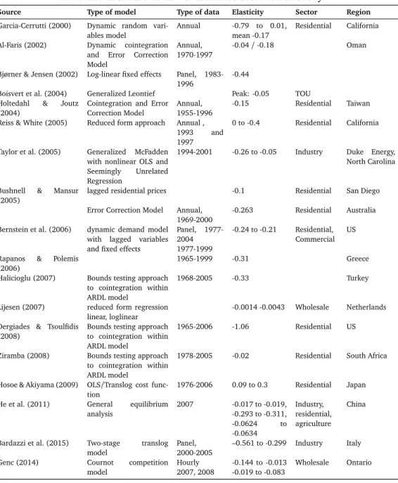
have estimated the elasticity for different sectors and time intervals. Table 2.1 shows

2 When Are Consumers Responding to Electricity Prices? An Hourly Pattern of Demand Elasticity

that estimates of price elasticity vary from -0.02 to -0.3 depending on the chosen ap- proach, the country-specific data and the sector. Taylor et al. (2005), for instance, find that short-run elasticity ranges from -0.05 to -0.26 for the industrial sector in North Carolina by using annual data. He et al. (2011) confirm this finding whereas Bardazzi et al. (2015) measure a slightly higher elasticity in terms of magnitude for the Italian industry sector. For the residential sector, numerous studies have been performed as well (i.e. Ziramba (2008), Dergiades & Tsoulfidis (2008) and Hosoe &

Akiyama (2009)). However, little attention has been devoted to the price response of the whole market with respect to wholesale prices. So far, this market has only been investigated by Genc (2014) and Lijesen (2007). Whereas Genc (2014) ap- plies a bottom-up Cournot modeling framework, Lijesen (2007) uses a regression approach in order to quantify the price elasticity during peak hours. Genc and Lije- sen conclude from their chosen approaches that the hourly price elasticity is rather small. They furthermore argue that in peak hours demand switching behavior of consumers barely occurs in practice.

In this article we extend the existing literature on short-run elasticity with respect to the wholesale price in two ways. First, we use wind generation as an instru- ment variable to solve the simultaneity problem of demand and supply.

Second, we account for the variation in utility from electricity consumption during the day.

Using hourly data on load, temperature, prices and wind generation for the German day-ahead market in 2015, we quantify the level of price elasticity and its variation throughout the day.

Our results show that the short-run price elasticity of demand in the German elec- tricity market is not perfectly inelastic. Even though our obtained short-run price elasticity of demand is generally low, consumers still react to price movements. Mea- suring the price elasticity of demand can give a more meaningful understanding of the contribution of demand reactions to system security. However, we stress that a price elasticity of demand with respect to the day-ahead price is not explicitly show- ing the contribution of each consumer group. The daily pattern of our estimate of price elasticity reveals some prominent peaks in the morning and evening, where the price elasticity of demand is highest. As expected, these hours show overall high price levels providing incentives to consumers for a reduction of their consumption.

In the morning and evening hours, price elasticity varies between -0.08 and -0.13.

Thus, we infer that demand adjustments in these hours are to some extent beneficial for consumers. On the contrary, we measure a lower price elasticity of demand at

1The approach is similar to Bönte et al. (2015).

8

2.1 Introduction

Table 2.1: Literature review of estimated short-run elasticity

Source Type of model Type of data Elasticity Sector Region

Garcia-Cerrutti (2000) Dynamic random vari- ables model

Annual -0.79 to 0.01, mean -0.17

Residential California Al-Faris (2002) Dynamic cointegration

and Error Correction Model

Annual, 1970-1997

-0.04/-0.18 Oman

Bjørner & Jensen (2002) Log-linear fixed effects Panel, 1983- 1996

-0.44

Boisvert et al. (2004) Generalized Leontief Peak: -0.05 TOU Holtedahl & Joutz

(2004)

Cointegration and Error Correction Model

Annual, 1955-1996

-0.15 Residential Taiwan

Reiss & White (2005) Reduced form approach Annual ,

1993 and

1997

0 to -0.4 Residential California

Taylor et al. (2005) Generalized McFadden with nonlinear OLS and Seemingly Unrelated Regression

1994-2001 -0.26 to -0.05 Industry Duke Energy, North Carolina

Bushnell & Mansur (2005)

lagged residential prices -0.1 Residential San Diego

Error Correction Model Annual, 1969-2000

-0.263 Residential Australia Bernstein et al. (2006) dynamic demand model

with lagged variables and fixed effects

Panel, 1977- 2004 1977-1999

-0.24 to -0.21 Residential, Commercial

US

Rapanos & Polemis (2006)

1965-1999 -0.31 Greece

Halicioglu (2007) Bounds testing approach to cointegration within ARDL model

1968-2005 -0.33 Turkey

Lijesen (2007) reduced form regression linear, loglinear

-0.0014 -0.0043 Wholesale Netherlands Dergiades & Tsoulfidis

(2008)

Bounds testing approach to cointegration within ARDL model

1965-2006 -1.06 Residential US

Ziramba (2008) Bounds testing approach to cointegration within ARDL model

1978-2005 -0.02 Residential South Africa

Hosoe & Akiyama (2009) OLS/Translog cost func- tion

1976-2006 0.09 to 0.3 Residential Japan He et al. (2011) General equilibrium

analysis

2007 -0.017 to -0.019, -0.293 to -0.311, -0.0624 to -0.0634

Industry, residential, agriculture

China

Bardazzi et al. (2015) Two-stage translog model

Panel, 2000-2005

–0.561 to -0.299 Industry Italy

Genc (2014) Cournot competition

model

Hourly 2007, 2008

-0.144 to -0.013 -0.019 to -0.083

Wholesale Ontario

night times and during the day. A lower elasticity indicates less willingness of con- sumers to adjust the consumption due to high or low electricity prices. This can be due to the fact that economic activity in general is higher during daytime.

The remainder of the paper is organized as follows. Section 2.2 deepens the un-

derstanding of supply and demand in electricity markets. Section 2.3 describes the

data and presents the applied econometric approach. Section 2.4 discusses the esti-

mation results. Section 2.5 concludes.

2 When Are Consumers Responding to Electricity Prices? An Hourly Pattern of Demand Elasticity

2.2 Measuring Market Demand Reactions Based on Wholesale Prices

In order to specify our econometric model capturing demand reactions due to elec- tricity wholesale price movements, knowledge about the supply and demand func- tions in electricity markets is pivotal. In this section, we therefore describe the func- tioning of the retail and wholesale electricity market before arguing that demand elasticity can be estimated based on market demand being defined as aggregated demand of all end consumer groups and wholesale electricity prices. We further specify the drivers of demand and supply by setting up the respective functions.

2.2.1 The Retail Market for Electricity

Consumers commonly sign contracts with retailers to take charge of their electric- ity demand. These contracts are subject to different possible tariff schemes ranging from time-invariant pricing to real-time pricing. Tariff structures vary depending on the consumer group and metering facilities.

Small end consumers (e.g. households, businesses, or small industries) in Germany are mostly on time-invariant tariffs. This means that the price of electricity for these consumer groups is at the same level for every hour over the entire year. These consumers therefore have little incentive to adjust their demand in the short-run. For larger consumers, such as big industrial companies, contracts are differently designed allowing them to benefit from adjust- ing consumption in the short run.

In Germany, the retail price that consumers pay for electricity consists of several components. The most important component is the price for electricity generation, which is the price that generators charge for the generation of electricity. Besides paying for the generation of electricity, end consumers also pay for the transmission and distribution of electricity, as well as for additional taxes and levies. In Germany, for instance the retail price consists of network charges, the renewable support levy, and taxes which are added to the wholesale price. Some of these additional price

2The electricity consumption of many end consumers is not observable over time because the metering facilities only display the amount of electricity consumed but not during which period measurement is performed.

3According to Bundesnetzagentur (2016), consumers can be grouped by their metering profile into customers with and without interval metering. Only consumers with interval metering have the technical capability to be billed depending on the time of usage. For Germany in 2014, 268 TWh were supplied to interval metered customers and 160 TWh to customers without interval metering.

10

2.2 Measuring Market Demand Reactions Based on Wholesale Prices

components vary substantially depending on the consumer group.

The differing retail prices for each consumer group lead to a total electricity demand of all con- sumers that varies over the year. This aggregated demand of all end consumers is equal to the observed load in the total electricity system.

2.2.2 The Wholesale Market for Electricity

The price for electricity generation is determined in the wholesale market. In prin- cipal, the wholesale market allows different players to place bids that eventually either result in produced quantities or demanded quantities for a specific point in time. Participants in these markets are for example utilities, retailers, power plant operators and large industrial consumers.

Figure 2.1(i) gives an exemplary overview of the five different players and their corresponding electricity demand and supply on the wholesale market. The first two players are two different utilities, A and B. As such, utility A and B illustrate cases for players with different generation assets while at the same time each of them pos- sesses different customer bases. However, for both utilities, we would expect that generation for their own customer base depends on the marginal cost of genera- tion. In other words, if the wholesale price is above the marginal cost of the utility’s marginal cost of generation, the utility chooses to supply their customer base instead of demanding quantities from the wholesale market.

The next player in the market we refer to is the retailer. As a retailer, supplying electricity is by default not an option and therefore we expect them to demand elec- tricity quantities only. The opposite is true for renewable and conventional genera- tion players. With marginal costs of zero, renewable generation players offer their production at very low cost compared to conventional generation players where marginal costs are greater than zero and vary depending on the generation technol- ogy.

Figure 2.1(ii) horizontally aggregates all demand and supply curves from each player we identified. It thus shows the aggregated demand and supply, as well as the realized equilibrium electricity price of 20 EUR

MWh.

Figure 2.1(iii) shows the resulting supply and demand bids by the individual play- ers in the wholesale market. First, players that can only supply electricity, such as renewable or conventional generators, appear in ascending order on the supply side

4In Germany, for example, electricity intensive industries are exempted from paying the renewable support levy.

2 When Are Consumers Responding to Electricity Prices? An Hourly Pattern of Demand Elasticity

0 20 40 60 80 Quantity [MWh]

40200 2040 6080 100

Price [EUR/MWh]

Utility A

0 20 40 60 80 Quantity [MWh]

Utility B

0 20 40 60 80 Quantity [MWh]

Retailer

0 20 40 60 80 Quantity [MWh]

Renewable Gen.

0 20 40 60 80 Quantity [MWh]

Conventional Gen.

(i) Wholesale market players

0 50 100 150 200

Quantity [MWh]

40200 2040 6080 100

Price [EUR/MWh]

(ii) Supply and demand aggregation

0 50 100 150 200

Quantity [MWh]

40200 2040 6080 100

Price [EUR/MWh]

(iii) Supply and demand in the wholesale market Figure 2.1: Electricity price formation on the wholesale market

only. Second, retailers demand quantities and generally more, if prices are low.

Third, players that own generation assets and also have customers, net their supply and demand positions internally before submitting bids. This is the case for utility A and B. The bids for the demand and supply side depend on the internal netting of supply and demand. In total this results in four possible outcomes for placing bids which can be describes as follows

•

sell bid on the supply side for generation units that have not been internally matched and could satisfy the demand of other participants

•

purchase bid on the demand side for demand that has not been internally matched

•

sell bid on the supply side, resulting from demand that has been matched internally but would be able to reduce consumption if the price rises above a given threshold (see e.g. demand of utility B with 90 EUR

MWh)

•

purchase bid on the demand side for generation units that have internally be matched but that would substitute their production if the price falls below their marginal costs of generation.

Whereas the first two outcomes are intuitively straightforward, outcomes three and four may seem counter intuitive at first. Due to the internal matching of sup- ply and demand, parts of the demand and supply curve that have been internally

12

2.2 Measuring Market Demand Reactions Based on Wholesale Prices

matched result in bids on the opposite side. By placing these bids, utilities can optimize their position and choose to substitute formally demanded quantities to supplied quantities or vice versa, above or below a certain wholesale price.

The supply and demand curves in Figure 2.1(ii) and 2.1(iii) look very different from a first glance, but both result in the same price for electricity and lead to the same allocation of resources. Nevertheless, both provide a very different impres- sion of the price responsiveness of the demand side. Based on Figure 2.1(ii) the demand side can be characterized as rather price inelastic. In the example, the level of demand would not change if prices stay within a range of 5 to 80 EUR

MWh. Fig- ure 2.1(iii) may however lead to the misleading conclusion that the demand side in electricity markets is rather price elastic. Within the submitted supply and demand bids at the wholesale market it is not possible to identify separate bids that actually stem from generators or actual consumers of electricity. It is therefore not possi- ble to estimate the demand elasticity of actual electricity consumers based on the curves observed in the wholesale market. In order to estimate the demand elasticity of the actual electricity consumers it is, however, possible to combine the wholesale equilibrium price with the total load observed.

2.2.3 The Interaction of Wholesale and Retail Markets

Within this article we are interested in the reaction of electricity demand to electricity prices. Because disaggregated load data for each consumer group with the respective retail prices are not available, we focus our attention on the interaction of total hourly demand and hourly wholesale electricity prices. Figure 2.2 shows the relation we are interested in for an exemplary hour. The blue line depicts the supply curve for electricity generation. The red line is the aggregated demand curve of all consumers for electricity consumption. Consumers pay an average retail price of p

, which is made up of the wholesale price for electricity (p

) and additional price components (c).

When we account for the effect of the additional price components, we obtain the demand function that is observable in the wholesale market (whol esal e d emand, red dashed line). The intersection of wholesale demand and wholesale supply leads to point A and determines the wholesale price p

, as well as the quantity consumed and produced q

. By inferring the relationship illustrated in Figure 2.2 and using the wholesale price and total electricity demand, we are able to estimate the point elasticity of the red dashed demand curve.

5In Germany, most additional price components are added to the wholesale price independent on the price level or quantity consumed.

2 When Are Consumers Responding to Electricity Prices? An Hourly Pattern of Demand Elasticity

Q p

wholesale supply c

retail demand wholesale

demand p

q

p

A

Figure 2.2: Supply and demand curves for one exemplary hour

The relations of the demand and supply curve in electricity markets are only vaguely sketched in Figure 2.2. In reality, demand is fluctuating over time due to varying utility levels throughout the day. The demand for electricity can be regarded as a function of various inputs and the relation can be written as

d

f

, H DD, time-of-the-day) , (2.1) where d

is the quantity consumed, p

is the wholesale price for electricity, H DD are heating degree days capturing the seasonality within the data. H DD measure the temperature difference to a reference temperature. The variable therefore captures the seasonal variation of electricity demand. For example, if outside temperature is low, heating processes consume more electricity compared to warmer weather conditions.

In addition, electricity consumption depends on the time of usage. This is mainly driven by the variation of the consumer’s utility function over the day.

Additional variables determining the level of demand, such as economic activity, may also alter demand but are assumed to be time-invariant on an hourly basis and within the considered time span. Therefore, we abstract from including additional variables for the demand side in the short run.

Like the demand function, the supply of electricity can also be regarded as a func- tion of multiple inputs with the wholesale price p

being one of them. We define the supply function as:

6The data in Section 2.4 reveals that this relation is true for Germany, however it may not be applicable to other countries. In warmer climates also cooling degree days (CDD) determine the demand for electricity.

14

2.3 Empirical Framework

s

g

p

, p

, r

, (2.2)

where s

is the quantity produced, p

is a vector of fuel prices and r is the production of variable renewable energy.

In electricity markets, the structure of the supply side is commonly represented by the merit order curve. It represents the marginal generation costs of all conventional (fossil) power plants. The shape of the curve mainly depends on the technologies being used for power generation and their respective fuel prices p

.

However, variable renewable electricity generation is becoming increasingly important within the generation portfolio. This is particularly true for the German market region.

Since renewable technologies do not rely on fossil fuel inputs to generate electricity, their fuel costs are close to zero. Additionally, its stochastic nature that is driven by wind speeds and solar radiation makes generation vary throughout time. We will later make use of the stochastic nature and by using wind generation as an instrument variable within our econometric model.

2.3 Empirical Framework

2.3.1 Data

Our data set consists of hourly data for 2015. We include hourly data for load, day- ahead-prices and the forecast of production from variable renewables for Germany.

In addition, HDD are calculated based on hourly temperatures that we obtain from the NASA Goddard Institute for Space Studies (GISS). Summary statistics for all variables are provided in Table 2.2.

Table 2.2: Descriptive statistics (for weekdays, without public holidays and Christmas time)

Variable Mean Std. Dev. Min. Max. Source

Load[GWh] 61.688 9.428 38.926 77.496 ENTSO-E

Wind Generation[GWh] 8.574 6.864 0.153 32.529 EEX Transparency Day-ahead price[EUR/MWh] 35.6 11.5 -41.74 99.77 EPEX Spot

Temperature[^◦C] 10.4 7.9 -6.3 34.6 NASA MERRA

Heating degree days[K] 10.1 6.9 0 26.3 NASA MERRA

The hourly load profile for Germany was taken from ENTSO-E. According to ENTSO- E, load is the power consumed by the network including network losses but ex-

7Common power plant types and fuels are hydro power, nuclear, lignite, coal, gas and oil.

2 When Are Consumers Responding to Electricity Prices? An Hourly Pattern of Demand Elasticity

cluding consumption of pumped storage and generating auxiliaries.

The load data includes all energy that is sold by German power plants to consumers.

Load there- fore is the best indicator on the level of demand in the German market area since almost all energy sold has to be transferred through the grid to consumers. Fig- ure 2.3(i) shows average hourly values for weekdays in the German market area in a box plot. The plot shows significant differences in the level for night hours (00:00-6:00, 19:00-00:00) compared to daytime. Also load peaks in the morning (9:00-12:00) and evening hours (16:00-18:00). Especially in the evening, variation in load levels is higher than at other times. The average load level is 62 GW and the maximum peak load is 77 GW in the early evening hours.

0 1 2 3 4 5 6 7 8 9 1011121314151617181920212223 Hour

0 10 20 30 40 50 60 70 80

Load [GWh]

(i) Load data based on ENTSO-E

0 1 2 3 4 5 6 7 8 9 1011121314151617181920212223 Hour

60 40 20 0 20 40 60 80 100

Price [EUR/MWh]

(ii) Electricity price from EPEX

0 1 2 3 4 5 6 7 8 9 1011121314151617181920212223 Hour

0 5 10 15 20 25 30 35

Wind generation [GWh]

(iii) Wind generation from EEX Transparency

0 1 2 3 4 5 6 7 8 9 1011121314151617181920212223 Hour

0 5 10 15 20 25 30

Solar generation [GWh]

(iv) Solar generation from EEX Transparency Figure 2.3: Hourly data for load, electricity price, wind and solar generation for 2015

We obtain the hourly day-ahead price for electricity from the European Power Exchange (EPEX) which is the major trading platform for Germany. Historically the day-ahead price has evolved as the most important reference price on an hourly level

8ENTSO-E collects the information from the four German transmission system operators (TSO) and claims that the data covers at least 91% of the total supply. These quantities may also be reflected in the day-ahead price which we can not account for.

9To a small amount load may also include energy that is sold from neighboring countries to the German market. These trade flows impact the domestic electricity price and load. However, we expect this impact to be rather small.

16

2.3 Empirical Framework

in the wholesale electricity market. The day-ahead market run by EPEX Spot is by far the most liquid trading possibility close to the point of physical delivery.

The price is determined in a uniform price auction at noon one day before electricity is physically delivered. We follow this perspective and use the day-ahead price as our reference price for electricity generation. Although not all electricity is sold through the day-ahead-auction, the price reflects the value of electricity in the respective hours and contains all available information on demand and supply at that specific point in time. Figure 2.3(ii) shows a box plot for the hourly day-ahead electricity price for each hour of the day. The average hourly day-ahead electricity price is at 36 EUR

MWh over the 24 hours time interval and for weekdays (without public holidays and Christmas time). The electricity price pattern is similar to the load pattern emphasizing the fact that higher demand levels tend to increase prices in the day-ahead market. Especially during peak times in the morning and evening one can observe higher standard deviations and peaking prices. Standard deviation over all hours is around 12 EUR

MWh.

Electricity generation from wind and solar power is taken from forecasts published on the transparency platform by the European Energy Exchange (EEX). These fore- casts result from multiple TSO data submissions to the EEX. Since they are submitted one day before physical delivery, they contain all information that is relevant for par- ticipants in the day-ahead market.

Figure 2.3(iii) and 2.3(iv) show box plots for electricity generation from wind and solar power. Due to weather dependent gen- eration volatility, we observe a larger amount of volatility in the hourly data. Wind generation varies steadily throughout the day with a small increase during the day.

Solar generation shows its typical daily pattern with no generation at night and peak generation values for midday.

The level of demand does not only depend on the electricity price which in return is partially influenced by generation from wind. We add temperature as an additional parameter to our investigation of electricity demand since the level of temperature is a main driver for the seasonal variation of demand. We compute a Germany wide average temperature based on the reanalysis MERRA data set provided by NASA (NASA, 2016). The hourly values are based on different grid points within Germany that are spatially averaged in order to obtain a consistent hourly value for Germany.

Based on the hourly temperature we derive HDD that are relevant for the seasonal

10In 2015 264 TWh have been traded in the day-ahead market, compared to 37 TWh traded in the continuous intraday market (EPEX Spot, 2016).

11We also considered taking the actual generation from renewables but reckon that the ex-ante fore- casts are reflecting the causal relationship in a better way since decisions made on the day-ahead market are based on forecast values.

2 When Are Consumers Responding to Electricity Prices? An Hourly Pattern of Demand Elasticity

variation of demand in electricity markets.

2.3.2 Econometric Approach

Due to the fact that the electricity price is endogenously determined by the inter- action of demand and supply, we choose a two-stage approach to solve the simul- taneity problem.

As we are interested in estimating the demand function (2.1), possible instruments affecting the price but not the level of demand have to be de- termined. Possible instruments can be found on the supply side in (2.2), where fuel prices ( p

) and the production of variable renewable energy (r ) are considered.

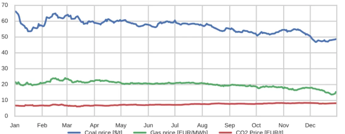
Although fuel prices are one of the major drivers for generation decisions, a closer look reveals that they show little variation over the year 2015 (see Figure 2.6 in the Appendix). Therefore, we exclude them from a further analysis within our frame- work.

The production of variable renewable energy (r) can further be split into wind (w) and solar (s) generation. Figure 2.4 depicts the respective correlations of renewable generation with prices and load for each hour interval of the day. In Figure 2.4i, we observe that the correlation between solar generation and load is higher in absolute values than the correlation between wind generation and load. However, wind and solar generation are correlated opposite in sign with load being positively correlated with wind generation and solar generation negatively correlated with load.

Figure 2.4ii shows the correlation between renewable generation and electricity price. Both, wind and solar generation are negatively correlated with the electricity price, however their patterns are different throughout the day. The correlation be- tween wind generation and electricity price weakens over the day until 17:00 where the correlation is lowest with an absolute value of -0.45. From 17:00 on the cor- relation between wind generation and price increases again. The pattern for the correlation between solar generation and electricity price is reversed whereas the increasing correlation until 17:00 is mainly driven by an increasing solar radiation.

Based on the generally high correlation of wind and prices and at the same time low correlation of wind and load, we choose wind generation as an instrument for the price.

12We calculate HDDs based on a reference temperature of 20^◦C.

13Durbin and Wu–Hausman test statistics show highly significant p-values. The null hypothesis tests for all variables in scope being exogenous. With p-values for both test of both equal to 0,000 we reject the null of exogeneity implying that prices and demand are endogenous.

14Statistically speaking, weak instruments may cause estimation bias if the correlation with the en- dogenous explanatory variable (in our casep^w_h,t) is very low.

18

2.3 Empirical Framework

0 5 10 15 20

Hour of the day 1.0

0.8 0.6 0.4 0.2 0.0 0.2 0.4

Correlation

WindSolar

(i) Correlations with load

0 5 10 15 20

Hour of the day 1.0

0.8 0.6 0.4 0.2 0.0 0.2 0.4

Correlation

WindSolar

(ii) Correlations with price Figure 2.4: Correlations with load and prices in 2015

More formally, wind generation as a variable fulfills the two conditions

(1) cov[w, p

0 and (2) cov[w,

0, where w is wind generation, p

the wholesale electricity price and

the error term of the general demand equation not to be confused with the error term

of equation (2.4). The first condition is needed in order to provide unbiased electricity price estimates. In our context the chosen instrument w correlates with the electricity price (see Figure 2.4(ii)). From the second condition it follows that w and

are not correlated.

Because wind can be regarded as a stochastic variable especially throughout the day and load inhibits strong daily patterns, both can be regarded as independent (see Figure 2.4(i)). With these two conditions fulfilled we are now able to postulate the first and second stage equations. The first stage can be written as

p

w

(2.3) and the second stage as

q

p

H DD

M ON

F RI

. (2.4)

We estimate price coefficients

and dummy coefficients

on an hourly basis h. We do this, because we expect the utility of electricity consumption to be different in each hour of the day. Here,

captures the price independent change of util- ity from electricity consumption throughout the day. Since we observe a different

15Testing for validity expressed bycov[w,µ] =0 within our framework is not feasible since our model is exactly identified.

2 When Are Consumers Responding to Electricity Prices? An Hourly Pattern of Demand Elasticity

demand pattern for working days and week-ends, we eliminate week-ends and hol- idays from the data. Furthermore, we add dummies for Monday (MON) and Friday (FRI)

to capture differing demand levels at the beginning and end of the working week. Based on our estimates, we can calculate the average hourly price elasticity of electricity demand according to

ε_h=

p

q

∂

q

∂

p

p

q

, (2.5)

where

is the hourly elasticity using the average price p

and average demand q

in the respective hour of the day (h).

2.4 Empirical Application

By applying the econometric framework, we are able to estimate the level of price elasticity of demand for the German day-ahead market on an hourly basis. The regression is based on levels and elasticity is calculated with respect to the average prices and quantities in each hour.

The results of the estimation can be found in Table 2.3. When taking a look at the price coefficients in Table 2.3(a), we can see that all price coefficients are negative in sign and are significant at least at the 1% level. We note that coefficients during morning hours (9:00-12:00) are lower in absolute values. The highest value can be found at 17:00. In this particular hour, a wholesale price increase of 1 EUR

MWh leads to a demand reduction of 201.8 MWh. The hourly dummy coefficients in Ta- ble 2.3(a) capture the varying level of utility throughout the day. During the day, hourly coefficients are higher than at other times. In the evening, we can observe a peak in the level of utility, especially between 16:00 - 20:00 (see Figure 2.5(i)).

Beside the hourly coefficients, we also account for the influence of temperature and weekdays on electricity demand. All coefficients are significant at the 0.1% level and can be explained in their sign. HDD have a positive sign and thus increase electric- ity demand. Mondays and Fridays are negative in sign, indicating that demand is generally lower at the start of the week and at the end compared to other working

16For Mondays the dummy is positive for the time between 0:00 and 9:00. For Fridays the time frame is from 17:00 to 23:00.

17In a previous version of the paper, we normalized our data to the median, which is why previous estimates differ from this version. Furthermore, elasticity was calculated with respect to the average price and quantity level including values of zero. As we are running a pooled regression many observations of zero were included which resulted in low estimates of the elasticity.

20

2.4 Empirical Application

days.

+RXURIWKHGD\

/HYHO>*:K@

p <0.01 p <0.02 p <0.05 p >0.05

(i) Hourly dummies

+RXURIWKHGD\

3ULFHHODVWLFLW\RIGHPDQG

p <0.01 p <0.02 p <0.05 p >0.05

(ii) Hourly price elasticity Figure 2.5: Hourly dummies and price elasticity of electricity demand in 2015

Since the focus of our work is on the hourly price elasticity of demand, we estimate the elasticity based on the results from the basic regression. The results are displayed in Figure 2.5(ii) and the numerical values can be found in Table 2.3(c).

As observed before, all coefficients are negative in sign and significant at a strict 1% level. With the elasticity estimates at hand, we are able to plot a distinctive pattern for the hourly price elasticity of demand for the German day-ahead market.

The unique shape of the hourly price elasticity of demand pattern is depicted above in Figure 2.5(ii). Our results show that demand reactions are rather small. How- ever, a perfect inelastic demand assumption can also be neglected. More precisely, the elasticity is the lowest during night times (22:00 - 6:00). During these hours electricity demand and utility from electricity consumption is generally lower (as we can also observe from Table 2.3(a)). The graph shows two prominent peaks of price elasticity of demand in the morning and in the evening. At these times working hours start and end. Possible reasons for a high elasticity of demand at those times is the shifting or delaying of consumption. When prices are low in the morning, some processes may be able to start the operation earlier and thereby circumventing a time with a higher electricity price level. The same might be true for the evening, when the workday ends. Here working hours may be extended to lower price levels at other times. Throughout the day, the price elasticity of demand remains relatively

18It is important to note that elasticity is calculated with respect to the wholesale price level and not the retail price level, as represented by the dashed red demand curve in Figure 2.2. The elasticity with respect to retail prices would be higher. For example if we consider the sum of additional price components (c) to be 150 EUR/MWh, which is an average value based on Eurostat (2016) for Germany, the highest elasticity measured would be -0.58 at hour 17:00-18:00. Without the sum of additional price components, we obtain an elasticity of -0.13 as indicated in Table 2.3(c).