E SSAYS ON THE ECONOMICS AND

E SSAYS ON THE ECONOMICS AND

REGULATORY DESIGN OF POWER SYSTEMS

Inauguraldissertation zur

Erlangung des Doktorgrades der

Wirtschafts- und Sozialwissenschaftlichen Fakultät der

Universität zu Köln 2015 vorgelegt

von

MSc ETH Simeon Hagspiel aus

March

Referent Prof. Dr. Felix Höffler

Korreferent Prof. Ulrich W. Thonemann, Ph.D.

Tag der Promotion 01.07.2016

Preface

Energy has been the focus of my interest since the first days of my engineering stud- ies at ETH Zurich starting in 2005. Nevertheless, having finished my Master’s the- sis in 2011, I was somehow unsatisfied with the level of specific knowledge I had reached. So it was quite clear to me that I needed to continue learning as a doc- toral student. However, it was not clear to me at all how much more I really had to learn. That I resolved to complement my engineering perspective with a doctoral thesis in economics did not really contribute to simplify the task. Even though I was able to draw on what I had learned so far, I had to start asking questions differently, and to broaden the foundation of my work based on economic principles. Thus, my decision inevitably brought along additional workload and frustration, but also inspiration and satisfaction. In fact, it has probably been exactly that shift of per- spective that had a significant, sustainably positive impact on my knowledge about energy and power systems in particular. Moreover, it probably affected the devel- opment of my soft skills in a very positive way, too. Overall, my years as a doctoral student at the University of Cologne were very enriching in several respects, and an experience I would not want to miss.

During this adventure, several people and institutions have supported me in dif- ferent ways, for which I am deeply grateful. First and foremost, I want to thank Felix Höffler for academic supervision and support. His clear line and typical man- ner of giving dry yet constructive comments forced and motivated me to reflect the existing, and tackle the continuation of my work. His high standards and degree of rationality were certainly reasons why I have learned so much rigorous economic thinking. I am also very grateful to Ulrich Thonemann for academic advice and com- ments as well as for being the second assessor of my thesis, and to Van Anh Vuong for chairing the defense of my dissertation.

An institutionally and financially stable framework has been provided by the In-

stitute of Energy Economics (EWI) and the University of Cologne, as well as by the

German Research Foundation (DFG) with the research grant HO5108 / 2-1 and the

German Federal Ministry for Economic Affairs and Energy (BMWi) and the German

Federal Ministry of Education and Research (BMBF) with their Energy Storage Ini-

tiative (grant 03ESP239).

persistent and enjoyable teamwork with my coauthors, Joachim Bertsch, Christina Elberg and Lisa Just. Much of the quality and fun is owed to these three people.

Special thanks also go to my student assistants Clara Dewes and Michael Franke for their scientific support. Furthermore, I was very lucky to have an exceptionally well- functioning, dynamic and pleasurable working environment at EWI (including man- aging directors, administration, IT, library, student assistants, research associates, as well as the nice cleaner who reminded me regularly that I should eventually go home in the evening).

Lastly, I am infinitely happy to have my two ladies Lisa and Chiara, as well as my family and friends.

Simeon Hagspiel Cologne, December 2015

Contents

Preface v

1 Introduction 1

1.1 Outline of the thesis . . . . 3

1.2 Discussion of methodological approaches . . . . 6

1.3 Concluding remarks . . . . 9

2 Spatial dependencies of wind power and interrelations with spot price dynamics 11 2.1 Introduction . . . . 11

2.2 Stochastic dependence modeling using copulas . . . . 14

2.2.1 Copulas and copula models . . . . 14

2.2.2 Conditional copula and simulation procedure . . . . 16

2.3 The model . . . . 17

2.3.1 The data . . . . 18

2.3.2 Derivation of synthetic aggregated wind power . . . . 20

2.3.3 Supply and demand based model for the electricity spot price 20 2.3.4 Estimation and selection of copula models . . . . 23

2.4 Results . . . . 26

2.4.1 Revenues and market value of different wind turbines . . . . . 28

2.4.2 Market value variations in Germany . . . . 29

2.4.3 The impact of changing wind power penetration levels . . . . 31

2.5 Conclusions . . . . 33

2.6 Appendix . . . . 35

3 Supply chain reliability and the role of individual suppliers 39 3.1 Introduction . . . . 39

3.2 Related literature . . . . 41

3.3 Supply chain reliability and the contribution of individual suppliers . 43 3.3.1 Supply chain reliability . . . . 43

3.3.2 The contribution of individual suppliers . . . . 44

3.4 Payoff scheme . . . . 51

3.4.1 Supply chain organization . . . . 51

3.4.2 Allocation rule . . . . 53

3.4.3 Investment incentives . . . . 55

3.5 Empirical case study: Wind power in Germany . . . . 58

3.5.1 Estimation procedure . . . . 58

3.5.2 Data . . . . 59

3.5.3 Results . . . . 60

3.6 Conclusions . . . . 64

3.7 Appendix: Data and preparatory calculations . . . . 67

4 Congestion management in power systems - Long-term modeling frame- work and large-scale application 73 4.1 Introduction . . . . 73

4.2 Economic framework . . . . 77

4.2.1 Setting I – First-Best: Nodal pricing with one TSO . . . . 79

4.2.2 Setting II: coupled zonal markets with one TSO and zonal re- dispatch . . . . 82

4.2.3 Setting III: coupled zonal markets with zonal TSOs and zonal redispatch . . . . 86

4.2.4 Setting IV: coupled zonal markets with zonal TSOs and gener- ator component . . . . 87

4.3 Numerical solution approach . . . . 87

4.4 Large-scale application . . . . 91

4.4.1 Model configuration and assumptions . . . . 92

4.4.2 Results and discussion . . . . 95

4.5 Conclusions . . . 100

4.6 Appendix . . . 102

5 Regulation of non-marketed outputs and substitutable inputs 113 5.1 Introduction . . . 113

5.2 The model . . . 116

5.3 Optimal regulation . . . 121

5.3.1 Preparatory analysis . . . 121

5.3.2 Full information benchmark . . . 123

5.3.3 Asymmetric information . . . 124

5.4 Comparing the optimal regulation to simpler regimes . . . 128

5.5 Conclusion . . . 131 5.6 Appendix . . . 133

Bibliography 139

1 Introduction

Power systems regulation is never at rest. [ ... ] [ T ] here are quieter periods and more active ones. Present times appear to demand a particularly active regulatory response.

Ignacio J. Pérez-Arriaga (2013) Power systems have been sparking public attention ever since the first central power plant was commissioned by Thomas Edison on Pearl Street, New York City, in September 1882. They have played an important role in the growth of economies worldwide, and will continue to do so in the future. As an inevitable consequence of public attention and societal importance, power systems have also been subject to intense scrutiny and debates about their best possible organization. After a pe- riod of private initiatives and competition at the end of the 19 ^th and the beginning of the 20 ^th century, the power sector was for a long time organized by means of vertically integrated monopolies. The entire supply chain – including production, transmission, distribution, and retailing – was hence comprised within a few elec- tric utilities that were either state-owned or private and subject to heavy regulation.

However, this paradigm has been overthrown by the deregulation wave beginning in the 1980ies, aiming at a reorganization of power systems to create far-reaching eco- nomic benefits. As a consequence, nowadays the production and retail sides of the supply chain typically involve numerous competitive firms. It is a recognized fact that if properly implemented, deregulation was indeed able to involve substantial improvements in the performance of power sectors (Joskow (2008b)).

Nevertheless, regulation remains at the core of power systems. Two of the most

important reasons for regulatory interventions to be present in today’s power systems

are negative environmental externalities from power generation, and the fact that

the power grid is a natural monopoly. The former reason has once more gained

momentum during the very recent UN Climate Change Conference in Paris. Indeed,

to implement the strategies the 195 parties have agreed upon, the supply side of the

power sector – with 25% currently the largest single source of global greenhouse

gas emissions – will be key for future developments (IPCC (2014)). It is and will

be a major challenge to design a regulatory framework for the power sector that

incentivizes and manages its transformation towards low-carbon power production (e.g., by means of renewable energies) in an effective and economically efficient way.

The other important reason for regulatory intervention stems from the natural monopoly characteristics of the power grid. Recent advances in the theory of reg- ulation make it imperative to rethink and redesign regulatory approaches for the power grid in order to reap efficiency gains. Especially in the light of the above mentioned fundamental changes in power systems, taking advantage of better reg- ulation gains even more importance. In fact, greenhouse gas emissions in the power sector and grid regulation are closely related when it comes to the expansion of vari- able renewable electricity sources (such as wind and solar), which typically requires expansion of the electricity network.

Generally speaking, getting the economics and regulation of power system right is important since weak designs may entail significant losses of social welfare. In fact, due to the large turnover of the power sector (e.g., around 455 bn. € in Eu- rope in 2013, representing more than 3% of European GDP ¹ ), even small relative inefficiencies cause a large absolute excess burden.

Against this background, it is the goal of this thesis to investigate some aspects of the economics and regulatory design of power systems. The focus lies on the above mentioned fields where regulatory intervention is particularly relevant and economically justified: The integration of variable renewable energies into power systems on the one hand, and electricity network expansion and operation on the other. Overlapping areas are also taken into account. As I will show in this thesis, these fields are promising candidates to yield substantial improvements when being reformed. To this end, novel approaches shall be suggested to identify and tackle economic and regulatory deficits and to improve the related outcomes. In the context of renewable expansion and grid regulation, my thesis contributes to the academic debate with the following four papers that are contained in Chapters 2-5. Three of those chapters are joint work with co-authors whose contribution I shall once more gratefully acknowledge here. If elaborated as joint work, all authors contributed equally to all parts of the corresponding paper.

1

The annual turnover of the European electricity sector can be estimated with a simple calcula-

tion based on 3101 TWh of net electricity production and an average price of electricity for end-

consumers of 0.147 €/kWh. European GDP in 2013 was 13520 bn. €(all numbers taken from

Eurostat (2015)).

1.1 Outline of the thesis

Chapter 2: Spatial dependencies of wind power and interrelations with spot price dynamics (with Christina Elberg). Published in the European Journal of Operational Research, Vol. 241 (1), pp. 260-272, 2015.

Chapter 3: Supply chain reliability and the role of individual suppliers. Forthcoming as EWI Working Paper, in preparation for submission to Management Science.

Chapter 4: Congestion management in power systems – Long-term modeling frame- work and large-scale application (with Joachim Bertsch and Lisa Just).

Published as EWI Working Paper 2015 / 03, Revised and resubmitted to the Journal of Regulatory Economics.

Chapter 5: Regulation of non-marketed outputs and substitutable inputs (with Joachim Bertsch). Published as EWI Working Paper 2015 / 06, in prepa- ration for submission to the International Journal of Industrial Organi- zation.

In the following Section 1.1, I will outline the contents of these four chapters and put them into context as well as into relation with each other. In Section 1.2, I discuss the methodologies that are applied in the different chapters. Section 1.3 concludes the introduction.

1.1 Outline of the thesis

In my thesis, I investigate several aspects of the economics and regulatory design of power systems. I focus on the production and transmission sectors (even though the contents of Chapter 5 may also be applied to the distribution sector). Along this part of the supply chain, I analyze different economic activities and how they should be organized in order to induce short- and long-term efficiency. The specific challenges I address in the first two papers stem from the time-varying and interdependent temporal and spatial distribution of production (especially, from variable renewable energies) and demand, while the latter two papers focus on the degree and exchange of information between different players in the supply chain.

Chapter 2 deals with the integration of variable renewable energies, especially

wind energy, into power systems. If wind and solar were to (only) receive the whole-

sale electricity price (and no subsidies via, e.g., fixed feed-in-tariffs), they would face

the challenge that their generation is highly correlated: on a windy day in northern

Germany, all wind generators along the coast are able to produce. For that reason, prices earned by renewables will typically be below the average price level. Hence, it may make sense to install renewable capacities where correlation with other pro- ducers is favorable, even if the place is less windy.

In this paper, we assess the market value of variable generation assets at different locations using a stochastic simulation model that covers the full spatial dependence structures of generation by using copulas, incorporated into a supply and demand based model for the electricity spot price. This model is calibrated with German data.

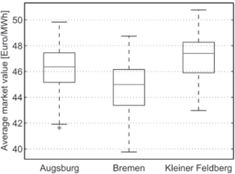
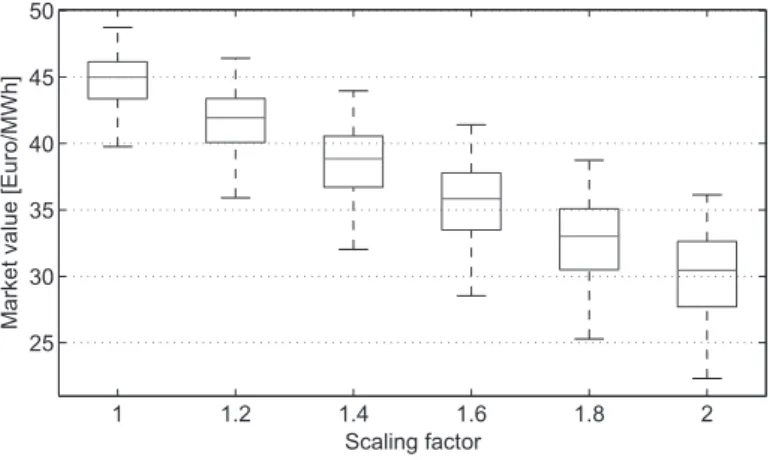
We find that the specific location of a wind turbine – i.e., its spatial dependence with respect to the aggregated wind power in the system – is of high relevance for its mar- ket value. It is reduced by up to 8 €/ MWh (i.e., 15%) compared to average spot price levels, and varies by up to 6 €/ MWh for the different locations that were ana- lyzed. Many of the locations show an upper tail dependence that adversely impacts the market value. Therefore, a model that assumes a linear dependence structure would systematically overestimate the market value of wind power in many cases.

This effect becomes more important for increasing levels of wind power penetration as the price effect of wind power becomes more pronounced.

Regulatory practice so far often ignores the complex dynamics and interactions of generation and electricity prices by offering, e.g., spatially and temporally fixed feed- in-tariffs. In contrast, to reveal the actual value of electricity at each specific time and place – needed to trigger incentives for efficient investments – the dynamics and interactions that are depicted in this section should be represented in the regulatory design of renewable energy integration.

Chapter 3 picks up a related issue arising from the stochastic nature of wind and solar generation. It analyzes the contribution of individual stochastic suppliers to the supply reliability of the overall system, as well as an appropriate payoff scheme.

How valuable an individual stochastic supplier really is for a given system is difficult to determine, since it not only depends on the stochastic nature of the individual supplier itself, but also on all other stochastic suppliers that are present. For reg- ulatory purposes, the contribution of intermittent renewables to system reliability is important because it should be the basis for any capacity payment to these gen- erators. In particular, it should influence the payments individual suppliers could receive in any sort of capacity mechanism that have been intensively discussed and implemented in many electricity markets.

To this end, I first investigate the statistical properties of the supply chain, includ-

ing stochastic and interdependent supply and demand. Based on these finding, I

1.1 Outline of the thesis

show that an efficient organization of the suppliers is difficult to achieve in a com- petitive environment (e.g., in the context of capacity mechanisms). To overcome this problem, I propose a payoff scheme based on marginal contributions and the Shapley value which may, for instance, be applied in a centralized procedure. The proposed concept exhibits desirable properties, including static efficiency as well as efficient investment incentives. In order to demonstrate the relevance and ap- plicability of the concepts developed, I investigate an empirical example based on wind power in Germany, thereby confirming my analytical findings. In practice, my approach could improve the design of capacity or renewable support mechanisms.

More generally, the approach could be applied to organize supply chains and their reliability more efficiently.

In Chapter 4, I turn my attention towards the impact of electricity generation, especially from renewable energies, on the electricity grid. Due to the fact that favorable sites for renewable electricity generation are typically far away from load centers, new grid infrastructures are often needed. However, as generation and grid services are unbundled in today’s liberalized power systems, it may be difficult to obtain a system outcome where planning and operational activities in the generation and grid sector are well coordinated. In this context, an appropriate regulatory design can help to improve or even resolve this coordination problem.

Key ingredient to organize the interaction between generation and grid is the way how congestion in the grid is managed. In principle, several congestion management designs are available, differing with respect to the definition of market areas, the reg- ulation and organization of grid operators, the way of managing congestion besides grid expansion, and the type of cross-border capacity allocation. In order to inves- tigate and compare the performance of different designs, we develop a generalized and flexible economic modeling framework based on a decomposed inter-temporal equilibrium model including generation, transmission, as well as their inter-linkages.

The model covers short-run operation and long-run investments and hence, allows to assess short and long-term efficiency.

Based on our modeling framework, we are able to identify and isolate implicit fric-

tions and sources of inefficiencies in the different regulatory designs, and to provide

a comparative analysis including a benchmark against a first-best welfare-optimal

result. Moreover, we provide quantitative results by calibrating and numerically

solving our model for a detailed representation of the Central Western European

(CWE) region, consisting of 70 nodes and 174 power lines. Analyzing six particu-

larly relevant congestion management designs until 2030, we show that compared to

the first-best benchmark, inefficiencies of up to 4.6% arise. Inefficiencies are mainly driven by the national organization of markets and responsibilities for the grid in- frastructures, which could be overcome by a coordinated European approach.

Chapter 5 takes a closer look at the specific activities in the grid sector itself, and investigates a problem that was neglected in the previous section: due to the fact that the electricity grid is a natural monopoly, the firm being in charge has its own (profit- maximizing) agenda and hence, needs to be regulated in order to align its activities with social preferences. This can be a challenging task if the firm has exclusive knowledge about the economic and technical characteristics of its activities which it is not willing to share voluntarily. For instance, in the case of electricity grids, the responsible firm may have multiple options to cope with an increasing deployment of renewable energy sources, such as grid expansion or improved grid operation.

At the same time, electricity systems are highly complex, and for the regulator it is often hard to observe and judge whether the mix and overall level of measures taken by the firm are adequate, let alone optimal.

This setting appears to be unresolved by the existing literature on regulation. We hence derive the theoretically optimal regulation strategy based on a menu of con- tracts that is able to make the firm reveal its exclusive knowledge. As an additional contribution, we then contrast our theoretical findings with other regulatory ap- proaches that are practically applied by regulatory authorities in many countries, even though they are seemingly simplistic and outdated from a theoretical perspec- tive. With this comparative analysis, we provide regulators with useful information about ways to improve their strategies. At the same time, we also show for the exem- plary case of Germany that the relatively simple (cost-based) regulatory approach may – under certain conditions – in fact be close to the theoretically optimal strategy.

1.2 Discussion of methodological approaches

Methodological approaches were chosen and developed to suitably address the spe- cific research question of each chapter. As discussed in Section 1.1, the specific challenges investigated in Chapters 2 and 3 stem from the interdependent tempo- ral and spatial distribution of supply (especially from variable renewable energies) and demand. Correspondingly, we apply statistical analysis and stochastic simula- tion models that are able to cover the stochastic nature of the underlying problem.

Interdependencies between the random variables are a main focus in both papers.

However, they are depicted in greater detail in Chapter 2, where copulas, i.e., full

1.2 Discussion of methodological approaches

multivariate dependence structures, are explicitly analyzed and modeled. In con- trast, Chapter 3 represents dependence structures based on covariance, i.e., a linear measure of dependence. Hence, Chapter 3 could be extended by covering general, non-linear dependence structures, possibly allowing for interesting additional in- sights. However, it should be noticed that the analytical tractability – which is indeed one of the main advantages and contributions of Chapter 3 – is probably jeopardized, or at least very complex.

Furthermore, it could be argued that the first two chapters appear to be some- what "incomplete". Indeed, they both conduct analyses of fundamental drivers on the supply side, especially regarding the availability of renewable resources. Both papers’ goal is to determine a system value for the product at hand (value of produc- tion in Chapter 2, and value of reliability in Chapter 3). Furthermore, both papers propose payoff mechanisms that are – in contrast to existing designs – in line with these system values, while inducing desirable properties, such as static efficiency and efficient investment incentives. However, even though many implications of these payoff schemes are thoroughly discussed, further analytical techniques could be ap- plied, such as optimization routines or game-theoretical equilibrium analysis. This would be a necessary and interesting next step in order to determine, e.g., the most promising business cases or the economic equilibrium under the suggested payoff schemes as well as possible deviations from a welfare-optimal benchmark.

The latter two papers (Chapters 4 and 5) both focus on the degree of information available to different firms in the system. Specifically, Chapter 4 focuses on informa- tion deficits stemming from the spatially aggregated uniform prices in zonal markets.

In this setting, asymmetric information is exogenously introduced at the interface between the production and transmission sector by means of different congestion management designs. Importantly, this information deficit cannot be resolved by the parties involved, such that the outcome is necessarily inefficient. The reason lies in the inherent incompleteness of aggregated uniform prices that do not represent real grid scarcities. Representing such an information deficit in a fundamental (par- tial) equilibrium model is not easy. In fact, classic equilibrium models build upon the assumption of perfect information for all market participants. Hence, in order to introduce this regulatory deficiency, we decompose our problem into the production and transmission sector and limit the amount of information that can be exchanged.

This is a novel methodological approach that was derived based on economic princi-

ples and proved to be applicable to large-scale problems while producing consistent

and robust results. For instance, we are able to confirm the economic inferiority

of zonal markets in comparison to nodal pricing that necessarily follows from the introduced information deficit. Nevertheless, it is fair to say that the methodology could benefit from further research. So far, neither the existence and uniqueness of a global optimum of the problem, nor the convergence of the solution algorithm have been analytically proven. Moreover, we build on the assumption of a perfectly regulated (i.e., cost-minimizing) firm responsible for the operation and expansion of the transmission sector. As such, we only consider information deficits induced by a flawed market design and disregard strategic withholding of information. While this isolation is indeed intended for this paper, its integration (especially on the trans- mission side) would represent an interesting extension. However, such an analysis would render the numerical solution even more complex, and would probably come at the cost of a higher level of abstraction to ensure numerical feasibility.

In a certain sense, the methodology of Chapter 5 is on the opposite side of the one applied in Chapter 4. It is a purely theoretical and highly stylized principle- agent model. Yet, it essentially considers a similar problem of information deficits between the involved parties (here, e.g., a monopolistic transmission firm and the regulator). However, in contrast to Chapter 4, the information deficit – even though also introduced exogenously – can here be resolved by means of a suitable contract framework. This endogeneity of information revelation is the reason why the frame- work is so complex (and interesting) to solve, and why the analytical analysis needs such a high level of abstraction.

Lastly, I shall mention that my entire thesis largely disregards the complexities of the retail sector, and instead assumes an inelastic demand in all chapters. There are essentially two reasons why this assumption is made: First, demand for electricity is indeed relatively inelastic, especially in the short-term. This is mainly due to large shares of consumers not being exposed to short-term price variations, rather paying a uniform price that only changes, e.g., once a year – even though consumers’ utility from consuming electricity is in fact often highly time-dependent (for instance, elec- tric lighting is an essential service that people are typically not willing to postpone).

Second, assuming an inelastic demand often facilitates the analytical and numerical

analysis and solution. For instance, it may under certain conditions allow to for-

mulate a non-linear welfare-maximization as a linear cost-minimization that can be

solved much more easily (as done in Chapter 4, for instance). Despite these reasons,

the inelastic demand assumption can be seen as a fairly strong assumption. Hence,

even though the analysis will quickly become complex, future research could relax

this assumption and introduce elastic demand functions.

1.3 Concluding remarks

1.3 Concluding remarks

Nearly all energy-related (research) questions can be posed and answered from dif- ferent perspectives, using different assumptions, methodologies and ways of inter- pretation. Unsurprisingly, energy-related research is hence conducted by several academic disciplines, among which the technical and economic sciences are proba- bly the ones that are involved the most. Moreover, interdisciplinary interfaces are often included or even crossed in order to embrace the full scope of a problem.

My thesis is primarily meant as a contribution in the field of energy economics, while in addition, some of the papers reach out to a generalized economic prob- lem and broader area of interest and application. ² It applies economic ideas and concepts, and provides novel approaches and insights regarding the economics and regulatory design of power systems. Specifically, it focuses on the efficiency of design alternatives, which serves as an objective analysis framework and basis of valuation.

While doing so, I largely take into account the technological features of the under- lying system, e.g., aspects of meteorology, technical functionalities of power plants, or Kirchhoff’s laws in power grids. In contrast, however, I focus less on aspects of equity, i.e., the question how resources could be distributed throughout society in a way that we consider to be fair. At the same time, I believe that one of the main future challenges in the energy sector will be to complement economically efficient designs with notions of equity. To this end, economic analysis could be joined by political and sociological approaches. As an example, let me mention the European discussion about nodal pricing. Even though many researchers have clearly argued in favor of a nodal pricing regime in terms of efficiency, it seems that (political) decision-makers have been avoiding serious consideration of this issue, perhaps due to a general aversion towards changes, but certainly also because an implementation would entail significant redistributional effects. It will be necessary yet challenging to overcome such barriers, e.g., by means of second-best approaches that still pro- vide a high level of economic efficiency while at the same time being politically feasible. ³ To this end, distributive effects will need to be taken into perspective to make efficient solutions work.

2

This mainly applies to the contents of Chapter 3 and 5. Both papers take power systems as an (important) exemplary area of application, but refer to more general issues (i.e., supply chain reliability in the former, and monopoly regulation in the latter paper).

3

In the mentioned example, it could for instance be interesting to only expose the supply side to nodal

prices, while retail prices remain uniform throughout the country.

2 Spatial dependencies of wind power and interrelations with spot price dynamics

Wind power has seen strong growth over the last decade and increasingly affects electricity spot prices. In particular, prices are more volatile due to the stochastic nature of wind, such that more generation of wind energy yields lower prices. There- fore, it is important to assess the value of wind power at different locations not only for an investor but for the electricity system as a whole. In this paper, we develop a stochastic simulation model that captures the full spatial dependence structure of wind power by using copulas, incorporated into a supply and demand based model for the electricity spot price. This model is calibrated with German data. We find that the specific location of a turbine – i.e., its spatial dependence with respect to the aggregated wind power in the system – is of high relevance for its value. Many of the locations analyzed show an upper tail dependence that adversely impacts the market value. Therefore, a model that assumes a linear dependence structure would systematically overestimate the market value of wind power in many cases. This ef- fect becomes more important for increasing levels of wind power penetration and may render the large-scale integration into markets more difficult.

2.1 Introduction

The amount of electricity generated by wind power plants has increased significantly during recent years. Due to the fact that wind power is stochastic, its introduction into power systems caused changes in electricity spot price dynamics: Prices have become more volatile and exhibit a correlated behavior with wind power fed into the system. In times of high wind, spot prices are observed to be generally lower than in times with low production of wind power plants. Empirical evidence of this ef- fect has been demonstrated for different markets characterized by high wind power penetration, e.g., by Jónsson et al. (2010) for Denmark, Gelabert et al. (2011) for Spain, Woo et al. (2011) for Texas or Cutler et al. (2011) for the Australian market.

Due to the cost-free availability of wind energy, wind power plants are characterized

by marginal costs of generation that are close to zero and therefore lower than those

for other types of power plants such as coal or gas. Hence – if the wind blows – wind power replaces other types of generation and thus leads to lower spot market prices in such hours. As a consequence, power plants are faced with increasingly difficult conditions and an additional source of price risk when participating in the market.

Until now, fluctuating renewable energy technologies (including wind power itself) have often been exempted from this price risk by support mechanisms (e.g., by fixed feed-in-tariff systems) in order to incentivize investments. However, their price risk draws more and more attention as they make up an increasing share of the genera- tion mix and may at some point be fully integrated in the liberalized power market.

Therefore, for an individual investor as well as for a social planner it becomes in- creasingly important to understand the value of wind generation and how it depends on the location of the wind turbine.

The purpose of this paper is to derive revenue distributions and the market value of wind power, i.e., the weighted average spot price wind power is able to achieve when selling its electricity on the spot market, at specific locations. It is clear that the value of a wind turbine at a specific location depends on whether it tends to produce when many other wind turbines at other locations can also produce, or whether it is one out of few producers at a given time. To capture the full stochastic dependence structure of wind power, we use copulas and incorporate the stochastic wind gen- eration in a supply and demand based model for electricity prices. More precisely, we take the following two steps. At first, we develop a stochastic simulation model for electricity spot prices that incorporates the market’s aggregated wind power as one of the determinants. We use the residual demand, given by the difference of to- tal demand and aggregated wind power, to establish the relationship between wind power and spot prices. Secondly, we link the market’s aggregated wind power to the wind power of single turbines in order to quantify their market value and the revenues depending on their specific location. We use copulas to model this inter- relation. The model is calibrated with German data, since Germany already has a high share of wind power.

We find that taking into account the entire spatial dependence structure is indeed

necessary, and that considering only correlations between a specific turbine and the

aggregate wind power would be misleading. Even if the correlation of a specific tur-

bine is lower compared to another, the resulting market value may be lower due to a

non-linear, asymmetric dependence structure. In fact, we find a pronounced upper

tail dependence that adversely impacts the market value for many of the locations

analyzed. Therefore, a model solely based on linear dependence measures would

2.1 Introduction

systematically overestimate the market value of wind power in many cases. More- over, it is shown that this effect becomes increasingly important for higher levels of wind power penetration.

Our paper contributes to three lines of literature. First, we complement the litera- ture on supply and demand based models. Within this class of models, Bessembinder and Lemmon (2002) were among the first to study the importance of demand and production costs for electricity prices. The model developed by Burger et al. (2006) follows a similar conceptual approach by including a non-linear functional depen- dence of the electricity spot price on a stochastic demand process as well as a long- term non-stationarity. Howison and Coulon (2009) further extend the number of state variables explaining the electricity spot price by including fuel prices. With our paper, we contribute to this line of literature by including stochastic produc- tion quantities of wind power that may impact the supply side and hence electricity prices.

Secondly, we extend the literature employing copulas, especially in the context of wind power applications. Copulas have first been identified by Papaefthymiou (2006) to be a suitable tool for modeling multivariate dependencies of wind speeds.

Subsequently, copulas have been employed in different studies to model spatial and temporal dependencies of wind speeds or wind power. Spatial dependencies have been modeled with the help of copulas by Haghi et al. (2010) for PV and wind power as well as system load in an Iranian case study, by Grothe and Schnieders (2011) for wind speeds in an optimization problem minimizing aggregated wind power fluctuations in Germany, by Hagspiel et al. (2012) for wind speeds in a Eu- ropean probabilistic load flow analysis, and by Louie (2014) for power generation from a multitude of pairs of wind turbines in order to identify the best-suited bivari- ate copula models. In contrast, copulas are used for temporal dependence structures in Pinson and Girard (2012) to model the multivariate stochastic process of short- term wind power trajectories (based on a methodology developed in Pinson et al.

(2009)) and in Zhou et al. (2013) to investigate wind power forecasting based on probabilistic kernel densities. We contribute to this second line of literature by apply- ing conditional copulas to model the dependence structure between specific turbines and the aggregated wind power. This approach allows us to specify and investigate interrelations between the physical characteristics of a wind turbine and electricity spot prices, and hence to value wind power assets more appropriately.

In fact, the valuation of power generation assets is the third line of literature our

paper complements. So far, research on the valuation of power generation assets

has mainly focused on conventional power (e.g., Thompson et al. (2004), Porchet et al. (2009) or Falbo et al. (2010)) and the optimization of hydro power schedules (e.g., García-González et al. (2007) or Densing (2013)). The relatively few papers that deal with the valuation of wind power is primarily based on historical data of wind power and day-ahead market prices (e.g., Green and Vasilakos (2012)). In a recent study presented by Girard et al. (2013), wind power predictability is assessed as a decision factor during the planning phase of a wind power project, showing that the financial loss due to imbalance costs induced by imperfect predictions only represents a low share of revenue in the day-ahead market. Even though they find that the aggregation of wind farms over large distances has an impact on the market value, they do not further elaborate on spatial dependencies. Our paper concentrates on this particular issue and shows that spatial dependencies are indeed crucial for the market value of wind power projects, especially for increasing penetration levels.

The remainder of this article is organized as follows: Section 2.2 provides a short introduction to copula modeling with a particular focus on conditional copula sam- pling which we apply in our model. The model itself is presented in Section 2.3.

Section 2.4 reports the results of the methodology applied to the case of wind power in Germany, namely the revenues and the market value of specific wind turbines.

Section 2.5 concludes.

2.2 Stochastic dependence modeling using copulas

In this section, we briefly discuss the modeling of stochastic dependencies with the help of copulas. A more detailed introduction is provided e.g., in Joe (1997), Nelsen (2006) or Alexander (2008). For a comprehensive literature review of the current status and applications of copula models, the interested reader is referred to Genest et al. (2009), Durante and Sempi (2010) and Patton (2012).

2.2.1 Copulas and copula models

A copula is a cumulative distribution function with uniformly distributed marginals

on [ 0, 1 ] . Sklar’s theorem is the main theorem for most applications of copulas,

stating that any joint distribution of some random variables is determined by their

marginal distributions and the copula (Sklar (1959)). The bivariate form of Sklar’s

theorem is as follows: For the cumulative distribution function F : R ² → [ 0, 1 ] of

any random variables X , W , with marginal distribution functions F

, F

, there exists

2.2 Stochastic dependence modeling using copulas

a copula C : [ 0, 1 ] ² → [ 0, 1 ] such that

F ( x , w ) = C ( F

( x ) , F

( w )) . (2.1) Sklar’s theorem also holds for the multivariate case of n > 2 dimensions. The cop- ula function is unique if the marginals are continuous. Conversely, if C is a copula and F

and F

are continuous distribution functions of the random variables X , W , then (2.1) defines the bivariate joint distribution function. From Sklar’s theorem, it follows that copulas can be applied with any marginal distributions. Particularly, marginal distributions may differ for each of the random variables considered.

In our application we are interested in the dependence structure of the market’s aggregated wind power W and a single turbine wind power X . The copula captures the complete dependence structure of X and W . The selection of an appropriate copula model can be made independent from the choice of the marginal distribution functions. Taking advantage of this, the joint distribution of W and X is determined in a two stage process: First, the marginal distribution functions F

and F

are determined, followed by the selection of the most appropriate copula model.

Copula functions are mostly determined in a parametric way. There are different types of parametric copula models that can be used to capture the pairwise depen- dence. In many applications – such as ours – it is particularly important to differ- entiate between symmetric or asymmetric, tail or no tail, and upper or lower tail dependence structures. Therefore, one can test several parametric copula models that are able to capture these characteristics: The Gaussian copula is symmetric and has zero or weak tail dependence (unless the correlation is 1). In contrast, the sym- metric Student-t copula has a relatively strong symmetric tail dependence. Whereas the Frank copula is another symmetric copula with particularly low tail dependence, Clayton and Gumbel copulas incorporate an asymmetric tail dependence. Lower tail dependence is captured by the Clayton copula, while the Gumbel copula incorpo- rates an upper tail dependence. ¹ These copulas are listed in Table 2.1.

The marginals u and v can be interpreted as F

(x ) and F

(w), respectively. Φ

denotes the multivariate normal distribution function with covariance matrix Σ and t

the multivariate Student-t distribution with ν degrees of freedom and covari- ance matrix Σ. The copula parameters can be estimated based on observed data by

1

Gaussian and Student-t copulas belong to the group of Elliptical copulas, whereas Frank, Gumbel

and Clayton copulas belong to the group of Archimedian copulas. For a more extensive discussion

of different copula families, see, e.g., Nelsen (2006)

Copula family Copula function C ( u, v )

Gaussian Φ

Φ

( u ), Φ

( v ) Student-t t

t

( u ) , t

( v )

Clayton max

u

+ v

− 1, 0

Frank

ln

1 + (

)(

)

e^−θ−1

Gumbel e

(

)

Table 2.1: Copula models

optimizing the log-likelihood function:

θ ˆ = max

θ

X

t

ln c ( F

( x

) , F

( w

) ; θ ) (2.2) where θ denotes the parameter vector and c the copula density. The selection of the most appropriate copula model can then be determined based on the Akaike Information Criteria (AIC).

2.2.2 Conditional copula and simulation procedure

Like any ordinary joint distribution function, copulas have conditional distribution functions. The conditional copula can be calculated by taking first derivatives with respect to each variable, i.e., for u = F

(x ) and v = F

(w) we have

C (u | v) = ∂ C (u, v)

∂ v and C (v | u) = ∂ C (u, v)

∂ u . (2.3)

For the application presented in this paper, there is one inherent advantage of using conditional copulas rather than sampling directly from the bivariate copula distribution: Samples can be conditioned on time series that may serve as inputs to the simulation procedure. The time series characteristics can thus be preserved during the simulation process. We use time series of the market’s aggregated wind power as an input variable for the spot price model.

We consider the stochastic processes ( X

)

and ( W

)

. F

t

( X

) , F

t

( W

) are uniformly distributed random variables on [0, 1]. For random variables U

, V

∼ U ( 0, 1 ) , F

¹

t

(U

) and F

¹

t

(V

) thus follow the distributions of X

and W

, respec-

tively. It is important to notice that by applying the inverse distribution functions,

the dependence structure is not influenced, i.e., U

and V

as well as F

(X

) and

F

(W

) have the same copula C .

2.3 The model

The conditional sampling procedure can be summarized as follows:

1. Apply the marginal distribution function F

to the time series of the market’s aggregated wind power ( w ₁ , w ₂ , w ₃ , ... ) in order to get v ₁

, v ₂

, v ₃

, ...

.

2. Simulate (u 1 , u ₂ , u ₃ , ...) from independent uniformly distributed random vari- ables.

3. For each observation F

t

( w

) = v

, apply the inverse conditional copula C

¹

Wt(Wt)

,F

·| v

to translate u

into u

by:

u

= C

Wt(Wt)

,F

u

| v

(2.4)

4. Apply the inverse marginal distribution functions to u

₁ , u

₂ , u

₃ , ...

in order to obtain the corresponding simulations of the random variable X

: €

F

¹

1

u

₁ , F

¹

2

u

₂ , F

¹

3

u

₃ , ... Š

.

2.3 The model

We develop a stochastic simulation model for the single turbine wind power and electricity spot prices, including a precise representation of their interrelations. The interrelation is established by the aggregated wind power that is related to both the electricity spot prices as well as the single turbine wind power. Hence, we set up a model that represents these two relationships: First, a supply and demand based model that takes, among others, the aggregated wind power as an input.

Second, a stochastic dependence model that links the single turbine wind power to the aggregated wind power. These two parts of the model can be summarized by the following two equations:

S

= h

(D

− W

) + Z

(2.5)

X

= F

¹

t

C

¹

X t(Xt),F_Wt(Wt)

U

| F

(W

)

(2.6)

where S

is the hourly stochastic spot price and X

the hourly single turbine wind

power, for t ∈ N . The spot price S

is determined by two components: First, the

function h

describes the dependence of the spot price on the residual demand that

is determined by the difference of the electricity demand level D

and the stochastic

aggregated wind power W

. Second, a short term stochastic component adds to the

spot price that is denoted by Z

. As operators of wind power plants are able to curtail

their power output in case of negative spot prices, their price is non-negative, i.e., S

= max { 0, S

} .

The second part of the model links the hourly single turbine wind power X

to the aggregated wind power W

. F

and F

denote the corresponding marginal distri- bution functions. The joint distribution function of these two random variables is de- termined by the corresponding copula, i.e., F

_,W

( x

, w

) = C F

( x

) , F

(w

)

. Due to the copula’s ability to separate marginal distribution functions and the de- pendence structure, the joint distribution function can be modeled in a two-step process: First, the marginal distribution functions F

and F

are determined.

Second, the appropriate copula C

X t(X_t)

,F

is selected and estimated. We deploy the conditional copula in order to keep the time series properties of the stochastic process (W

)

. For the simulation procedure, independent [ 0, 1 ] -uniformly ran- dom variables U

are needed. Note that the marginal distribution functions are the same within a month m, i.e., F

= F

if i, j ∈ m. The same holds for F

, h

and C

X t(X_t)

,F

.

Based on Equations (2.5) and (2.6), the amount of hourly wind power produced by a single turbine and the spot prices can be simulated. We sample from these model equations using a Monte Carlo simulation (n = 10000) in order to investigate the market value and revenue distributions as well as the relevance of the dependence structure with the aggregated wind power for single turbines at different locations.

While the revenue is simply the sum of the products of electricity generation and prices, the market value of a wind turbine is the average spot price weighted with the electricity generation of the respective wind turbine:

M V = P

t

X

S

P

t

X

. (2.7)

In the following subsections, we explain the input parameters and the different parts of the model in more detail.

2.3.1 The data

Different data sets are deployed in order to calibrate and estimate the different parts

of the model. In the following, we explain the content and origin of these sets, as

well as the way in which the data are preprocessed.

2.3 The model

Expected and realized generation by the German aggregated wind power:

For the supply and demand based model (represented by h

in Equation (5)), data is needed on the effectively delivered day-ahead prognosis of the German aggregated wind power in 2011. Note that the day-ahead prognosis – and not the actual aggre- gated wind power – is used, since this is the relevant information for the day-ahead market (Jónsson et al. (2010))). In contrast, for the estimation of the appropriate copula (C ) the realized generation of 2011 is used in order to determine its depen- dence structure with the realized single turbine wind power at different locations.

Expected as well as realized generation data are provided by the transmission sys- tem operators and published on the EEX Transparency Platform (EEX Transparency Platform (2012)).

Wind speeds of single stations: Hourly mean wind speeds for various stations in Germany are provided via the national climate monitoring of the German Weather Service for the years 1990-2011 (DWD (2014)). The measurement data for 19 lo- cations are used in this project to determine the corresponding power output series of wind turbines. ² Wind speeds are scaled to the hub height of currently installed wind turbines (100 meters) assuming a power law: v

= v

(h 1 /h 0 )

, where h ₀ is the measurement height, h ₁ the height of interest and α the shear exponent. Ac- cording to Firtin et al. (2011), α is assumed to be 0.14.

Wind power capacities: The development of currently installed wind power ca- pacities per federal state between 1995 and 2011 is available from the German Wind Energy Association (German Wind Energy Association (BWE) (2012)). In 2011, in- stalled wind power capacities in Germany amounted to 27.1 GW.

Electricity demand levels: Hourly electricity demand levels for the German mar- ket in 2011 — used as one of the explaining variables for spot prices and denoted by D

in Equation (2.5) — are provided by ENTSO-E (2012).

Spot prices: EPEX day-ahead prices from 2011 are deployed for the calibration of the spot price model (Equation (2.5)). The EPEX day-ahead market is organized by an auctioning process that matches supply and demand curves once a day, thus determining prices at which electricity is exchanged in each respective hour.

2

Missing data are interpolated based on the previous and next available value if the missing gap is

not exceeding 12 hours. If the gap is longer, the values are replaced by data of the same station

and same hours of the previous year.

2.3.2 Derivation of synthetic aggregated wind power

As an important input for the model, curves are needed that describe the wind power that the currently installed wind power capacities would have produced during the last decades (i.e., the long-term stochastic behavior of aggregated wind power in the power system). In the model, the curve is needed for the estimation of the marginal distribution F

of the aggregated wind power W

. It is important to notice that this curve has to be derived synthetically, as wind power capacities changed significantly during the last years.

Based on wind speeds and wind power capacities, the synthetic German aggre- gated wind power is generated as follows: By applying a power curve capturing the characteristics of the transformation process from wind energy to electrical power, wind turbine power generation profiles can be derived. In this study, the power curve is assumed to be one of a GE 2.5 MW turbine (General Electric (2010)). Alter- natively, one could use an average taken from multiple turbines. The transformation is based on a look-up table derived from the power curve and linear interpolation.

Furthermore, electrical output is determined as a ratio of installed wind power ca- pacity (i.e., scaled to [ 0, 1 ] ). Multiplying this ratio with the wind power capacity installed in the corresponding federal state yields the wind power. The above steps are repeated for 16 locations (one for each federal state) and all available years (1990–2011), resulting in a time series for what would have been produced during the last 22 years with current wind power capacities. In order to check the plausibil- ity of this approach, historical wind energy time series and volumes can be compared to the model estimates. The comparison for the 2011 time series yields high con- formity with an R ² of 0.84. Another check of consistency is done by calculating the accumulated aggregated wind power production volumes for the past 10 years from the synthetically generated curves, and comparing them to the overall wind power production as reported in Eurostat (2012). We find the deviations to be less than 12%.

2.3.3 Supply and demand based model for the electricity spot price

We develop a supply and demand based model to derive electricity spot prices de-

pendent on the level of wind power. A similar approach has been applied in Burger

et al. (2006). The main difference between our and their approach is that we use

the residual demand instead of total demand. We are therefore able to integrate the

effect of wind power on spot prices.

2.3 The model

We describe the non-linear relation between residual demand and spot prices (i.e., h

in Equation (2.5)) by an empirical function estimated from historical hourly spot prices, demand and wind power data. To derive a functional form for h

we use spline fits which are suitable to capture the non-linearities in the demand-price de- pendence. The parameters of h

are estimated from historical data for the reference year 2011 on a monthly basis in order to capture seasonal differences and variations on the supply side that occur, e.g., because of planned outages or variations in fuel costs.

30 40 50 60 70

20 0 20 40 60 80 100

Residual demand [GW]

Price [Euro/MWh]

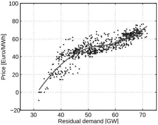
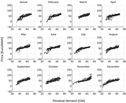
Figure 2.1: Demand-price dependence in February 2011 and spline fit

Note that if demand were totally price-inelastic, the function h

would approxi- mate the supply curve that represents all available sources of electricity generation ranked in ascending order of their marginal generation costs (excluding wind en- ergy) that is often referred to as the merit order. Even though the electricity is generally very inelastic in the short term, there may be some price-response of de- mand. Hence, our function h

should not be seen as an unbiased estimator of the merit order.

The data and the corresponding spline fit are shown in Figure 2.1 for the month of February 2011. All other months of 2011 are presented in Figure 2.10 in the Appendix. As can be observed, the dependence between residual demand levels and prices is characterized by steep ends and a comparatively flat part in between (i.e., for the residual demand ranging between 40 and 70 GW). The steeper part in the lower tail is generally more pronounced than the price increase for higher residual demand levels. Rather moderate price increases in the upper tail may be interpreted by prevailing excess capacity in the German power market, leading to very few instances at which scarcity prices occur.

Besides the functional dependence on (residual) demand, additional stochastic

factors influence spot market prices such as speculation, unplanned power plant outages or scarcity prices or demand side management. These effects are lumped together and captured by the residual price process Z

in Equation (2.5). In the following, we aim at finding a model for Z

that is capable of capturing the charac- teristics observed in the data. We can derive the observed residual price component based on h

, the observations of residual demand and spot prices from z

= s

− h

, and use the result for the calibration of the residual price process (Z

)

. The time series z

is visually observed to be stationary within the considered time frame, which is confirmed by an augmented Dickey-Fuller test that indicates that the null hypothesis of a unit root can be rejected at the 95% level.

The empirical auto-correlation function of z

decays slowly, however, with an ap- parent dependence at a lag of 24 hours. We therefore choose to model Z

as a seasonal ARIMA (SARIMA) model with a 24 hour seasonality. In order to do so, the ARIMA model needs to be extended to include non-zero coefficients at lag s, where s is the identified seasonality period. SARIMA models can be specified in a multiplica- tive form, resulting in a more parsimonious model than simply extending ARIMA to s lags.

As the Engle’s ARCH test indicates that there is conditional heteroscedasticity in the data, we extend the SARIMA by a GARCH component. GARCH-type models are able to capture conditional heteroscedasticity by splitting the error term ε

into a stochastic component η

and a time-dependent standard deviation σ

. The latter can then be expressed dependent on lagged elements of ε and σ

(Engle (1982), Bollerslev (1986)).

Various specifications of SARIMA-GARCH models are estimated and evaluated.

Based on the AIC, a GARCH(1,1)-SARIMA(2,0,2) × (1,0,1) ₂₄ model is found to per- form best. The inclusion of additional parameters hardly improves the fit. Note that no constant needs to be added to the model of Z

due to the fact that the process has been already centered by applying a spline fit.

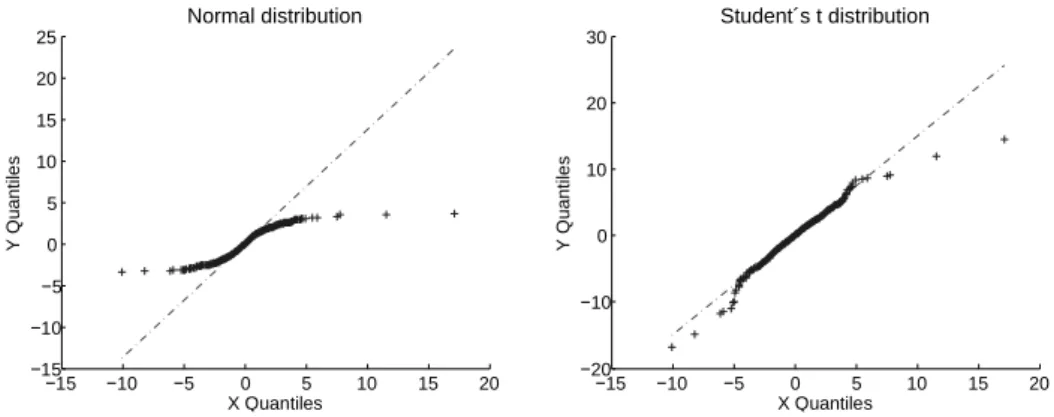
Comparing the residual’s distribution to the normal distribution yields unsatisfac-

tory results (Figure 2.2, left hand side). Thus, alternatively, the error term can be

specified as a t-distribution which leads to an improved match of the distributional

shapes (Figure 2.2, right hand side). Instead of η

∼ N (µ , σ ² ) we therefore use

η

∼ t (ν) , with ν being the t-distribution’s degrees of freedom that are estimated

from the data.

2.3 The model

15 10 5 0 5 10 15 20

15 10 5 0 5 10 15 20 25

X Quantiles

Y Quantiles

Normal distribution

15 10 5 0 5 10 15 20

20 10 0 10 20 30

X Quantiles

Y Quantiles

Student´s t distribution

Figure 2.2: QQ-plots of the 2011 residuals compared against a normal distribution and a Student-t distribution

Written explicitly, the model for Z

now takes the following form:

Z

=φ 1 Z

+ φ 2 Z

+ Φ 1 Z

+ Φ 1 (φ 1 Z

− φ 2 Z

) (2.8) + ε

+ θ 1 ε

1 + θ 2 ε

2 + Θ 1 ε

24 + Θ 1 (θ 1 ε

25 − θ 2 ε

26 )

ε

=σ

η

(2.9)

σ ²

=α + β 1 ε ²

₁ + γ 1 σ ²

₁ (2.10)

η

∼ t (ν) (2.11)

The parameters for the above model are estimated from the time series z

by optimizing the log-likelihood function. The estimates are presented in Table 2.2.

Parameter φ

φ

Φ

θ

θ

Θ

α β

γ

ν

Estimate 0.37 0.36 0.97 0.57 0.07 -0.85 2.96 0.30 0.47 3.61 Std. Error 0.15 0.12 0.00 0.15 0.02 0.01 0.03 0.03 0.27 0.16

Table 2.2: Parameter estimates for the residual price process model

2.3.4 Estimation and selection of copula models

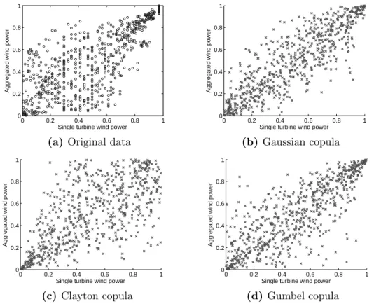
In this section, we select and estimate models for the joint distribution of a single turbine wind power and the German aggregated wind power for 19 wind power sta- tions in Germany ³ . We apply the two-stage process introduced in Section 2.2: First,

3

We determine the models for the joint distribution functions between the German aggregated wind

power and the following stations: Aachen, Angermünde, Augsburg, Bremen, Dresden, Emden,

Erfurt-Weimar, Idar-Oberstein, Kahler Asten, Kleiner Feldberg, Konstanz, Leipzig-Halle, Magde-

burg, Münster-Osnabrück, Oldenburg, Potsdam, Rostock, Saarbrücken and Schleswig.