Universally optimal crossover designs for the estimation of mixed-carryover effects with an application to biosimilar development

(1)

SFB 823

Discussion Paper

Johanna Mielke, Joachim Kunert

Nr. 3/2018

(2)

(3)

mixed-carryover effects with an application to biosimilar development

Johanna Mielke · Joachim Kunert

Received: date / Accepted: date

Abstract Biosimilars are medical products that are developed as copies of already established, large molecule drugs (biologics). For gaining approval, sponsors have to confirm that the proposed biosimilar has the same efficacy and safety as the originator product. This comparability exercise includes also, in most cases, that large clinical trials are conducted in patients. However, even with the evidence gained during the clinical studies, there is still some uncertainty if patients who were already treated with the originator can be switched to the biosimilar or if even multiple switches between the biosimilar and the originator are acceptable. A simple way to address the question of switchability is the estimation of so-called mixed and self-carryover effects, which are carryover effects that not only depend on the treatment in the current period, but also on the treatment in the previous period. In this paper, we determine universally optimal designs for the estimation of mixed-carryover effects in a linear model with treatment, period, subject and self-carryover as nuisance parameters.

Keywords biosimilars·self carryover effects·mixed-carryover effects·crossover design·switchability

The authors gratefully acknowledge the funding from the Deutsche Forschungsgemeinschaft (SFB 823), from the European Union’s Horizon 2020 research and innovation programme under the Marie Sklodowska-Curie grant agreement No 633567 and from the Swiss State Secretariat for Education, Re- search and Innovation (SERI) under contract number 999754557. The opinions expressed and arguments employed herein do not necessarily reflect the official views of the Swiss Government.

Johanna Mielke

Novartis Pharma AG, Basel, Switzerland Tel.: +41613245702

Fax: +41613243039

E-mail: johanna.mielke@udo.edu Joachim Kunert

Department of Statistics, University of Dortmund, Germany

(4)

1 Introduction

A biosimilar (the test product) is developed as a copy of an already approved large molecule drug, a so-called biologic (the reference product). Market authorization is granted after the sponsor of the biosimilar has shown the comparability of the test and the reference products at the analytical, non-clinical and clinical level (CHMP, 2014). If a biosimilar gains approval, it has been confirmed that patients who are taking the biosimilar can expect the same treatment effect and the same safety profile as patients who are taking the reference product.

Biosimilars are still a fairly new concept with the first biosimilar approved in Eu- rope in 2006 (Omnitrope, Sandoz) and the first biosimilar approved in the USA in 2015 (Zarxio, Sandoz). Even though there are by now already 36 approved biosimilars in Europe (Generics and Biosimilars Initiative, 2017a) and 7 approved biosimilars in the USA (Generics and Biosimilars Initiative, 2017b) and many more are expected to gain market authorization in the next years, there is still some uncertainty if patients who were already treated with the reference product can be switched to the biosimilar or even if multiple switches are allowed. This would mean that the au- tomatic substitution of the reference product by the biosimilar at the pharmacy level could be possible. The practice of switching at the pharmacy level is mostly accepted for generics. For biosimilars, the positions of regulatory agencies are diverse: for example, regulators in Finland state that ”switches between biological products are common and usually not problematic” (Finnish Medicines Agency, 2015) while the regulatory agency in Ireland ”does not recommend that patients are switched back and forth between a biosimilar and the reference medicinal product” (Health Prod- ucts Regulatory Authority, 2015).

Additional evidence might be required to support the decision as to whether single or multiple switches between a biosimilar and its reference product should be permit- ted. This evidence could be provided by an additional clinical study that is conducted specifically for analysing the impact of single or multiple switches on the treatment success. A simple statistical methodology for showing the impact of switching between a biosimilar and its reference product could be based on the direct estimation of the impact of switching by calculating the so-called mixed and self-carryover effects.

This idea was first proposed by Afsarinejad and Hedayat (2002). They introduced a model in which the usual carryover effect that only depends on the treatment in the previous period is replaced by two different carryover effects per treatment. These carryover effects do not only depend on the treatment in the previous period, but also on the treatment in the current period: if both treatments are different, a mixed- carryover effects is introduced, if the treatment are the same, a self-carryover effect is used. In the case of two treatments, the proposed model is identical to the inclusion of interactions between the direct effects and carryover effects. From previous parallel groups trials, it will generally be known prior to the assessment of switchability that the direct effects of the two treatments can be considered similar. From previous long term experiments (where subjects receive either reference or test over several periods) it will also be known that the self-carryover effects can be considered to

(5)

be identical. However, for claiming switchability, we might want to confirm that the mixed-carryover effects have equal values. Hence, it is necessary to perform a study which uses a design that allows the estimation of the mixed-carryover effects.

It is generally desirable to use a study design which is as efficient as possible.

While for the showing of biosimilarity, mostly parallel groups designs were conducted in the past (Mielke et al, 2016), such designs are clearly not appropriate for the assessment of switchability because one or multiple switches have to be included in the study design. So far, not many switching studies have been published and there is currently no well-established standard for the choice of the study design. In this paper, we determine universally optimal designs for the estimation of mixed-carryover effects in the case of two treatments (the test and the reference product) in a linear model with treatment, period, subject and self-carryover effects as nuisance parameters. This work builds on results by Kunert and Stufken (2002) and Kunert and Stufken (2008) who studied optimal designs for the estimation of the treatment effect when period, subject and both self and mixed-carryover effects are nuisance parameters. We study efficient designs for the joint estimation of self and mixed-carryover effects in a separate paper.

The rest of the paper is structured as follows: in Section 2, we introduce the necessary notation that is used in Section 3 for identifying the optimal designs. In Section 4, we compare the derived optimal designs with designs used in practice. In Section 5, we investigate if the designs can be improved by including periods without any treatment. We summarize our results in Section 6.

2 Notations and definitions

We consider the model that was described in Kunert and Stufken (2002) and Kunert and Stufken (2008). We assume that the responseyu,r of subjectu(u=1, ...,n) in periodr(r=1, ...,p) can be written by

yu,r= (

α_u+β_r+τ_d(u,r)+ρ_d(u,r−1)+eu,r ifd(u,r)6=d(u,r−1) αu+βr+τ_d(u,r)+χd(u,r−1)+e_u,r ifd(u,r) =d(u,r−1), whered(u,r)gives the treatment of subjectuin periodr,α_uis the subject effect of subjectu,β_r is the period effect in periodr,τ_iis the treatment effect of treatmenti, ρ_i is the mixed-carryover effect of treatmentiandχ_i is the self-carryover effect of treatmenti. The residual erroreu,ris assumed to be independent and identically dis- tributed with expectation 0 and varianceσ². To simplify the notation, we setσ²=1.

The set of all designs witht treatments,n subjects andp periods is denoted as Ωt,n,p. Here, we focus on the case of two treatments (Test - T, Reference - R;t=2) andp>2. Using the notation of Kunert and Stufken (2002), we define the matrices U=I_n⊗1_p(subject effect),P=1_n⊗I_p(period effect),T_d (treatment effect),M_d (mixed-carryover effects) andS_d (self-carryover effect), where⊗denotes the Kro- necker product,I_m is the identity matrix of dimensionm and1_m is a vector with

(6)

lengthmthat only contains the entries 1.

The goal of this analysis is to derive the characteristics of a designdthat is universally optimal for the estimation of the mixed-carryover effects in the class of design Ω2,n,p. Universally optimal is a term introduced by Kiefer (1975). If all information matricesC_dhave row sums and column sums 0, then a designd^∗is universally optimal if its information matrixC_d^∗is completely symmetric and the design maximises the trace ofC_dover alld∈Ω2,n,p. A matrixAis called completely symmetric if it can be written in the form

A=aI+b11^T,

wherea andbare real numbers. The information matrix for the estimation of the mixed-carryover effects is given by

C˜_d=M^T_dω^⊥([P,U,T_d,S_d])M_d,

whereω^⊥(A) =I−A(A^TA)⁻A^T is the projection on the space of all vectors that are orthogonal to the columns ofAand whereA^T gives the transpose andA⁻the g- inverse ofA. It can be easily confirmed that all information matrices ˜C_dhave column and row sums 0: for that, defineq=

0 1p−1

. Then, we observe that

M_d1₂+S_d1₂=Pq⇒M_d1₂=Pq−S_d1₂∈im([S_d,P])⊂im([T_d,S_d,U,P]), whereim(A)gives the image of matrixAand the first equality holds because each subject experiences a mixed or a self-carryover effect in all periods except in the first period. With that, we know that

ω^⊥([T_d,S_d,U,P])M_d1₂=0,

which directly leads to the conclusion that the column sums and row sums of ˜C_d= M^T_dω^⊥([P,U,T_d,S_d])M_dare 0. Therefore, the concept of universally optimal is applicable.

3 Identification of universally optimal designs

The strategy presented in this paper for identifying universally optimal designs follows the ideas of Kunert and Stufken (2002) and Kunert and Stufken (2008) and consists of two main steps: first, a matrixC_dthat is larger in the Loewner sense than the information matrix ˜C_d is derived (Section 3.1). Then, an upper bound for the trace ofC_dis determined and a class of designs is identified that reaches this bound (Section 3.2).

(7)

3.1 An upper bound for the information matrix

In this section, we derive an upper bound for the information matrix ˜C_din the Loewner sense. Since ˜C_dhas row and column sums 0 and is completely symmetric, we can multiply the information matrix from both sides with a matrixB₂∈R^2x2which has diagonal elements 1/2 and off-diagonal elements−1/2 without changing the matrix and we have the equality

C˜_d=B^T₂C˜_dB₂= (M_dB₂)^Tω^⊥([P,U,T_d,S_d])(M_dB₂).

The upper bound of the information matrix is obtained by removing the period effect from the information matrix. More concrete, we use Proposition 2.3 in Kunert (1983) which states that

C˜_d≤(M_dB₂)^Tω^⊥([U,T_d,S_d])M_dB₂=C_d, say, (1) which equality if and only if

(M_dB₂)^Tω^⊥([U,T_d,S_d])P=0. (2) Then, as shown in Kunert and Martin (2000), it is possible to use the following de- composition of the information matrixC_d:

C_d=C_d11−C_d12C⁻_d22C^T_d12−(C_d13−C_d12C⁻_d22C_d23) (C_d33−C^T_d23C⁻_d22C_d23)⁻(C_d13−C_d12C⁻_d22C_d23)^T, where, in the situation of this paper,

C_d11=B₂M^T_dM_dB₂−1

pB₂M^T_dUU^TM_dB₂, C_d12=B₂M^T_dT_d−1

pB₂M^T_dUU^T_dT, C_d13=B₂M^T_dS_d−1

pB₂M^T_dUU^TS_d, C_d22=T^T_dT_d−1

pT^T_dUU^TT^T_d, C_d23=T^T_dS_d−1

pT^T_dUU^TS^T_d, C_d33=S^T_dS_d−1

pS^T_dUU^TS^T_d.

In order to use the reduced information matrix stated in Equation (1), it is necessary to show that the condition stated in Equation (2) is fulfilled. We first note that there is always a dual-balanced design among the optimal designs. A sequence sis called dual to a sequences⁰ if sequencescan be changed to sequences⁰by in- terchanging the two treatments (e.g., TRTR, dual sequence: RTRT). A design d is dual-balanced if it uses sequencesexactly as often as sequences⁰. It is noteworthy that dual-balanced designs fulfill all conditions stated in Kunert and Stufken (2002)

(8)

(in each period, all treatments appear equally often, the mixed carryover effects of all treatments appear equally often, the self carryover effects of all treatments appear equally often) and we can therefore directly use the results obtained in Kunert and Stufken (2002). We refer to the conditions stated in Kunert and Stufken (2002) as conditions(∗). For showing that Equation (2) holds, we first rewrite the equation:

(M_dB₂)^Tω^⊥([U,T_d,S_d])P=B₂M^T_dω^⊥(U)P−C_d12C⁻_d22T^T_dω^⊥(U)P

−(C_d13−C_d12C⁻_d22C_d23)(C_d33−C^T_d23C⁻_d22C_d23)⁻ (T^T_dω^⊥(U)P−C_d23C⁻_d22S^T_dω^⊥(U)P).

From Kunert and Stufken (2002), we use thatT^T_dω^⊥(U)P=0 and B₂M^Tω^⊥(U)P=0

for the designs which fulfill conditions(∗), i.e., for all dual-balanced designs, which simplifies the term to

(M_dB₂)^Tω^⊥([U,T_d,S_d])P=−(C_d13−C_d12C⁻_d22C_d23)(C_d33−C^T_d23C⁻_d22C_d23)⁻ (−C_d23C⁻_d22S^T_dω^⊥(U)P).

The matricesC_d22 andC_d23 have column sums 0 (Kunert and Stufken, 2002) and as these matrices are in addition completely symmetric, they are a multiple ofB₂. Therefore, we can replace

C_d22=k₂₂B₂, C_d23=k₂₃B₂. Furthermore, asB₂is idempotent,

B⁻₂ =B₂. This leads to

(M_dB₂)^Tω^⊥([U,T_d,S_d])P=−(C_d13−C_d12(k₂₂B₂)⁻k₂₃B₂) (C_d33−(k₂₃B₂)^T(k₂₂B₂)⁻k₂₃B₂)⁻ (−k₂₃B₂(k₂₂B₂)⁻S^T_dω^⊥(U)P)

=−(C_d13−C_d12k23

k₂₂B₂)

C_d33−k23

k₂₂B₂ −

−k₂₃ k22

B₂S^T_dω^⊥(U)P

=0,

where the last equality uses that B₂S^T_dω^⊥(U)P=0 (Kunert and Stufken, 2002).

Therefore, we only need to determine sequences which maximise the trace of the matrix

C_d= (M_dB₂)^Tω^⊥([U,T_d,S_d])M_dB₂.

(9)

3.2 Maximising the trace ofC_d

Since the column sums ofC_d11,C_d12andC_d13 are 0 because of the multiplication byB₂, we are in the same setting as in Proposition 2 in Kunert and Martin (2000) and can therefore use the same strategy to find the optimal design. Letx,y∈Randl be an equivalence class of sequences which consists of a specific sequencesand its dual-balanced sequences⁰. Since we are in the two-treatment case and we consider only dual-balanced designs,Ω2,n,pconsists of 2^p−1different equivalence classes. Let π_dl be a vector of length 2^p−1which gives the proportion of sequences of the design dwhich belongs to thelth equivalence class. We use from Kunert and Stufken (2008) that for any designd∈Ω2,n,p,

tr(C_d)≤n·min

x,y 2^p−1

∑

l=1

πdlh_l(x,y) =:q^∗_d, with

h_l(x,y) =c11(l) +2xc₁₂(l) +x²c22(l) +2yc₁₃(l) +y²c33(l) +2xyc₂₃(l), where, in our situation,

c₁₁(l):=tr(B₂M^T_uw^⊥(U_u)M_uB₂) =tr(B₂(M^T_u(I−U_u(U^T_uU_u)⁻U^T_u)M_u)B₂)

=tr

B₂

M^T_uM_u−1

pM^T_uU_uU^T_uM_u

B₂

=tr

B₂

M^T_uM_u−1

pM^T_uU_uU^T_uM_u

,

c12(l):=tr(B₂M^T_uw^⊥(U_u)T_u) =tr

B₂

M^T_uT_u−1

pM^T_uU_uU^T_uT_u

,

c13(l):=tr(B₂M^T_uw^⊥(U_u)S_u) =tr

B₂

M^T_uS_u−1

pM^T_uU_uU^T_uS_u

, c₂₂(l):=tr(B₂T^T_uw^⊥(U_u)T_u) =tr

B₂

T^T_uT_u−1

pT^T_uU_uU^T_uT_u

, c₂₃(l):=tr(B₂T^T_uw^⊥(U_u)S_u) =tr

B₂

T^T_uS_u−1

pT^T_uU_uU^T_uS_u

, c₃₃(l):=tr(B₂S^T_uw^⊥(U_u)S_u) =tr

B₂

S^T_uS_u−1

pS^T_uU_uU^T_uS_u

.

In these equations,M_u,U_u,T_u,S_uare the design matrices for theuth subject of the mixed-carryover effects, the subject effects, the treatment effects and the self-carryover effects, respectively. Due to the properties ofπ_dl (non-negative,∑²

p−1

l=1 π_dl =1), it is clear that

2^p−1

∑

l=1

π_dlh_l(x,y)≤max

l h_l(x,y) which leads to

tr(C_d)≤min

x,y max

l h_l(x,y).

(10)

Letx^∗,y^∗be values such that max

l h_l(x^∗,y^∗)≤max

l h_l(x,y).

Following Kunert and Stufken (2008), we defineL^∗as the set of equivalence classes with

l∈L^∗if and only ifh_l(x^∗,y^∗) =max

µ hµ(x^∗,y^∗).

As in previous publications, the main technical difficulty is to identify numbersx^∗,y^∗ and optimal classes of sequencesl∈L^∗. In the derivation of optimal designs for the estimation of the direct treatment effects in the presence of mixed and self-carryover effects as nuisance parameters (two treatments, Kunert and Stufken, 2008), the task was massively simplified because it was possible to show that the function h_l is, at the optimal values x^∗,y^∗, independent of the choice of the equivalence class l^∗. Unfortunately, this trick is not applicable in our case. Therefore, we optimizex^∗,y^∗ and the optimal classes of sequencesl∈L^∗simultaneously. It is important to note that since the terms c_{i j}(l) are invariant for a sequence and its dual sequence and therefore are invariant for all sequences within one equivalence class, we represent an equivalence classl, without loss of generality, with a sequencesthat ends with treatment T. For example, if TRT and RTR are the dual sequences of equivalence classl, we focus on the sequences=T RT. In the following we introduce additional notation which is required for the identification of optimal designs. For that, letn_j(s) be the number of appearances of treatment T (j=1) or R (j=2) in the sequence s, ˜n_j(s)is the number of appearances of mixed-carryover effects andt_{p j}(s)is 1 if treatment jis in the last period and 0 otherwise. With that notations, it follows that for everys, there is exactly one jsuch thattp j(s) =1 and it is 0 in all other cases.

The number of appearances of self-carryover effects is given by

¯

n_j(s) =n_j(l)−n˜_j(s)−t_{p j}(s).

It is necessary to distinguish between the sequences that start with treatment T and the sequences that start with treatment R. In the first case, if ñ₁(s)is the number of mixed-carryovers for treatment T, the number of mixed carryovers for treatment R is ñ2(s) =n˜1(s). If the treatment sequence starts with an R, the number of mixed carryovers for R is ñ2(s) =n˜1(s) +1. Using this notation, it is possible to derive simpler terms forci j(see Appendix) and this allows the simplification of the function h_l. In our situation, for the special case of two treatments, we can write the function h_l as

hl,1(x,y) =n˜1(s) 1−2x−y²−2xy +n²₁(s)

−2x² p −2y²

p −4xy p

+n₁(s)

2x²+2y²+2y²

p +4xy+2xy p

+

−y² 2 −y²

2p−y²−2xy

(11)

in case the sequencesstarts withT and as h_l,2(x,y) =n˜₁(s) 1−2x−y²−2xy

+n₁(s)² −2x²

p −2y² p −4xy

p

+n1(s) 2x

p +2y

p +4xy+2x²+2y²

+ 1

2− 1

2p−2x−y−y²−2xy

in case the sequencesstarts withR. It is noteworthy that the trace of the information matrix is completely determined byn₁(s)and ˜n₁(s). Therefore, these are the parameters that need to be identified for the determination of the optimal design. The following new proposition is the main tool for the identification of optimal sequences in the case of designs with an odd number of periods.

Proposition 1 Let p be an odd number. Then, for sequences starting and ending with the same treatment, the upper boundary of the trace ofC_d, q^∗_d, is attained by

x^∗= p

p+1, y^∗=− p p+1 and

n^∗₁(s) = p+1

2 ,n˜^∗₁(s) = p−1 2 .

Proof The proof consists of three main steps: first, we start with a pair of characteristics of the sequences,n₁(s)and ˜n₁(s), that we consider to be optimal. In the next step, we determine optimal valuesx^∗,y^∗for this choice and confirm afterwards that our choice ofn₁(s)and ˜n₁(s)was indeed optimal.

For that, we consider sequencesswith the characteristics n^∗₁(s) = p+1

2 and ˜n^∗₁(s) = p−1 2 .

Next, the corresponding optimal values of x,y should be determined. The partial derivatives ofh_l,1(x,y)with respect tox,yare given by

dh_l,1(x,y)

dx =−2 ˜n1(s)−2yn˜1(s)−4x

pn1(s)²−4y

p n1(s)²+4xn₁(s) +4yn₁(s) +2yn₁(s)

p −2y, dh_l,1(x,y)

dy =−2yn˜₁(s)−2xn˜₁(s)−4y

pn₁(s)²−4x pn₁(s)² +4yn₁(s) +4yn1(s)

p +4xn₁(s) +2xn1(s) p −y−y

p−2y−2x.

(12)

Settings these equations equal to 0, we note that all values ofyand x^∗= p

p+1 are optimal. In the following, we set

y^∗:=− p

p+1 =−x^∗.

In the direction ofx, the second derivative is positive, i.e., there exists only one minimum in the direction ofx. The function is constant in the direction ofy. Therefore, we have identified a global minimum. Including our knowledge in the functionh_l,1 leads to

h˜_l,1:=h_l,1(x^∗,y^∗) = n˜₁(s)

(p+1)²+ p²−p 2(p+1)².

This function appears to be independent of the appearance of treatment T (n₁(s)is not present in the formula), but this is not the case: the appearance of the treatments influences the range of possible mixed-carryover effects and therefore indirectly still influences the choice of optimal designs.

In the third step, we need to confirm that our choice ofn₁(s),n˜₁(s)was indeed optimal. For this, it is sufficient to confirm that the derived function ˜h_l,1is maximal for

n₁(s) = p+1

2 and ˜n₁(s) = p−1 2 .

We only need to confirm optimality at the point of the identified valuesx^∗,y^∗, since this is already the minimum of the functionh^∗_l(x,y)with respect tox,y. The derived function ˜h_l,1clearly shows that choosing ñ₁(s)as large as possible is optimal. The largest value for a sequence starting and ending with T is ñ₁(s) = ^p−1₂ . This choice directly determines thatn1(s) = ^p+1₂ which completes the proof. ut For the chosen values of mixed-carryover effects ñ₁(l^∗), the function ˜h_l,1simpli- fies to

h˜_l^∗_,1= p²−1

2(p+1)². (3)

Proposition 1 only refers to sequences which uses the same treatment in the first and in the last period. Therefore, it is necessary to confirm that starting with a different treatment than the one used in the last period cannot improve the design in the case of an odd number of periods.

Proposition 2 Let p be an odd number. Then,

hl,2(x^∗,y^∗)<h_l^∗,1(x^∗,y^∗),

where l^∗is the equivalence class with a sequence s with n^∗₁andn˜^∗₁as given in Propo- sition 1. The values x^∗ and y^∗ are the real numbers which were also identified in Proposition 1.

(13)

Proof Evaluating the functionh_l,2atx^∗,y^∗leads to h˜_l,2=2pn˜₁(l) +p³−p²−p−1

2p(p+1)² .

It is necessary to compare the value of ˜h_l,2to the value of the function ˜h_l^∗_,1which is given in Equation (3) atx^∗,y^∗and therefore to confirm that

p²−1

2(p+1)² >2pn˜₁(l) +p³−p²−p−1

2p(p+1)² ⇔0>2pn˜₁(l)−p²−1

⇔n˜< p 2+ 1

2p

The number of mixed-carryovers, ˜n₁(l), cannot be larger than ₂^p. Therefore, this con-

dition always holds true. ut

Combining Proposition 1 and Proposition 2, we have now identified optimal sequences in designs with an odd number of periods. Next, we focus on designs with an even number of periods.

Proposition 3 Let p be an even number and p>2. Then, for sequences with different treatments in the first and last period (start with R, end with T), the upper boundary of the trace ofC_dis reached for

x^∗= p−1

p , y^∗=−1−p p and

n^∗₁(s) = p

2, n˜^∗₁(s) = p−2 2 .

Starting with the same treatment that is used in the last period cannot increase this value, i.e.,

hl,1(x^∗,y^∗)<h_l^∗,2(x^∗,y^∗).

Proof Very similar to the proof of Proposition 1 and 2. See the Appendix for details.

3.3 Example

The analysis in the previous section showed that for designs with an odd number of periods, only sequences should be used in which the subjects switch after each period and the starting and ending period should be the same. For example for 5 periods, this restricts our attention to sequencess=T RT RT,s⁰=RT RT R. If the number of periods is even, the subjects should again switch between T and R after each period, but the treatment in the first and in the last period should be different. For 6 periods, this leads to the sequencess=RT RT RT,s⁰=T RT RT R. As optimal designs have to be dual-balanced, the sequencessands⁰have to be appear equally often.

(14)

4 Study designs in practice

It is interesting to see how these optimized study designs relate to study designs which are applied for switchability assessment of biosimilars in practice. As an example, we discuss the study design of the EGALITY study (Griffiths et al, 2017). It is important to note that the aim of this section is not to criticize the study design of the EGAL- ITY study: a study design is always optimized for a specific analysis method and the analysis of mixed-carryover effects, for which the designs we identified in this paper are optimal, was not one of the analyses conducted for the EGALITY study. We also acknowledge constraints in the choice of designs in practice due to, for example, operational constraints and expectations of health authorities (e.g., the recommended design to assess interchangeability (the term used by the health authority in the US for switchability) as stated in the FDA’s draft guidance (FDA, 2017)). However, we find it nonetheless interesting to compare the theoretical optimal designs with the designs applied in practice.

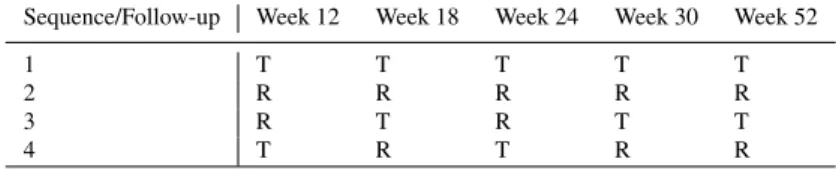
The EGALITY study was conducted in patients with moderate to severe chronic plaque-type psoriasis. 531 patients were randomised 1:1 to ErelziR (the biosimilar) or EnbrelR (the reference product). The study design is given in Table 1. In the following, we ignore that the time intervals between the follow-ups are not equidistant and consider each follow-up assessment as one period.

Table 1 Study design of the EGALITY study (Griffiths et al, 2017). T is the test treatment, R is the reference treatment.

Sequence/Follow-up Week 12 Week 18 Week 24 Week 30 Week 52

1 T T T T T

2 R R R R R

3 R T R T T

4 T R T R R

The trace of the information matrix for the study design used in the EGALITY study is 0.8636 (assuming one subject per sequence). The optimal design identified in this paper had a much larger trace of the information matrix (1.3333) and is clearly superior for the estimation of mixed-carryover effects. The much lower value of the criterion for the EGALITY study is due to the fact that half of the subjects (the subjects in the non-switching sequences) do not contribute much to the precision of the estimation of the mixed-carryover effects. Although the EGALITY study was clearly not tailored for the estimation of mixed-carryover effects, this shows the potential of using optimized designs.