Doubly Robust Estimation of Causal Effects with Multivalued Treatments

IHS Economics Series Working Paper 297

June 2013

Doubly Robust Estimation of Causal Effects with Multivalued Treatments

S. Derya Uysal

Impressum Author(s):

S. Derya Uysal Title:

Doubly Robust Estimation of Causal Effects with Multivalued Treatments ISSN: Unspecified

2013 Institut für Höhere Studien - Institute for Advanced Studies (IHS) Josefstädter Straße 39, A-1080 Wien

E-Mail: o ce@ihs.ac.at ffi Web: ww w .ihs.ac. a t

All IHS Working Papers are available online: http://irihs. ihs. ac.at/view/ihs_series/

This paper is available for download without charge at:

https://irihs.ihs.ac.at/id/eprint/2207/

Doubly Robust Estimation of Causal Effects with Multivalued Treatments

S. Derya Uysal

297

Reihe Ökonomie

Economics Series

297 Reihe Ökonomie Economics Series

Doubly Robust Estimation of Causal Effects with Multivalued Treatments

S. Derya Uysal June 2013

Institut für Höhere Studien (IHS), Wien

Institute for Advanced Studies, Vienna

Contact:

S. Derya Uysal

Department of Economics and Finance Institute for Advanced Studies Stumpergasse 56

1060 Vienna, Austria.

: +43/1/599 91-156 email: uysal@ihs.ac.at

Founded in 1963 by two prominent Austrians living in exile – the sociologist Paul F. Lazarsfeld and the economist Oskar Morgenstern – with the financial support from the Ford Foundation, the Austrian Federal Ministry of Education and the City of Vienna, the Institute for Advanced Studies (IHS) is the first institution for postgraduate education and research in economics and the social sciences in Austria. The

presents research done at the Department of Economics and Finance and aims to share “work in progress” in a timely way before formal publication. As usual, authors bear full responsibility for the content of their contributions.

Das Institut für Höhere Studien (IHS) wurde im Jahr 1963 von zwei prominenten Exilösterreichern –

dem Soziologen Paul F. Lazarsfeld und dem Ökonomen Oskar Morgenstern – mit Hilfe der Ford-

Stiftung, des Österreichischen Bundesministeriums für Unterricht und der Stadt Wien gegründet und ist

somit die erste nachuniversitäre Lehr- und Forschungsstätte für die Sozial- und Wirtschafts-

wissenschaften in Österreich. Die

bietet Einblick in die Forschungsarbeit der

Abteilung für Ökonomie und Finanzwirtschaft und verfolgt das Ziel, abteilungsinterne

Diskussionsbeiträge einer breiteren fachinternen Öffentlichkeit zugänglich zu machen. Die inhaltliche

Verantwortung für die veröffentlichten Beiträge liegt bei den Autoren und Autorinnen.

Abstract

This paper provides doubly robust estimators for treatment effect parameters which are defined in multivalued treatment effect framework. We apply this method on a unique data set of British Cohort Study (BCS) to estimate returns to different levels of schooling. Average returns are estimated for entire population, as well as conditional on having a specific educational achievement. The analysis is carried out for female and male samples separately to capture possible gender differences. The results indicate that, on average, the percentage wage gain due to higher education versus any other lower educational attainment is higher for highly educated females than highly educated males.

Keywords

Multivalued treatment, returns to schooling, doubly robust estimation

JEL Classification

C21, J24, I2

Comments

Supported by funds of the Oesterreichische Nationalbank (Anniversary Fund, project number: 14986)

Contents

1 Introduction 1

2 Econometric Method 3

3 Monte Carlo Evidence 9

4 Empirical Study 11

4.1 Data ... 11 4.2 Empirical Results ... 15

5 Conclusion 18

References 20

A Proofs 25

B Tables: Monte Carlo Evidence 28

C Tables: Empirical Study 31

D Figures 37

1 Introduction

Estimation of the causal effects of a binary treatment under the conditional in- dependence assumption has been studied extensively in the program evaluation literature (see for example Wooldridge 2007, Heckman et al. 2007, Imbens 2004, Rosenbaum & Rubin 1983, among others). While the literature dealing with the bi- nary treatment variables is comprehensive, the discussion on multivalued treatment variables is more recent and sparse. Given that in many empirical applications the programs which are being evaluated offer more alternatives than just one possible treatment the methods dealing more general treatment effect regimes are partic- ularly valuable. For example, from policy makers point of view it is usually more preferable to get information on the causal effects of different labor market programs rather than just looking at the effect of participating in any one of the programs versus not participating. Similarly, the effects of different doses of a drug or, as in this paper, the effects of different levels of educational attainment might be more interesting than just looking at the binary cases.

This study provides a simple method to estimate the causal effects of a multival- ued treatment variable which possesses a property known as double robustness. In general, doubly robust methods combine two estimations methods each of which estimates the same parameter(s) of interest but uses different model specifications.

Thus, doubly robust methods require both models specifications. The advantage of using both model specifications is that the parameter(s) of interest can be con- sistently estimated even if one of the model specifications is wrong which is not the case when the methods are used alone.

In other words, using doubly robust methods provides the practitioners more chances to get consistent estimators. Since in most of the applied works it is not possible to determine whether the model is correctly specified or not, having a doubly robust estimator for the parameter of interest might be quite useful. The method proposed here is closely related with the method used by Hirano & Imbens (2001) for the binary treatment case. We gener- alize the doubly robust estimator they are using for the potential outcome model with a multivalued treatment variable. The asymptotic distribution of the general- ized doubly robust estimator is derived based on the results by Wooldridge (2002) and Wooldridge (2007). Additionally, the small sample properties of the proposed method and the underlying single methods are evaluated by a small Monte Carlo study. The interest of the simulation experiment lies on the demonstration of the double robustness property of the combination method under misspecified models as well as comparison of the small sample properties under correct model specifications.

Furthermore, the doubly robust method is applied on the unique data set of British Cohort Study to estimate the returns to different levels of schooling.

Although this study is related to the several papers in different branches of the lit- erature, it also differs from the existing literature in many ways. The interest on

1

For further discussion on double robustness see Robins & Rotnitzky (1995), Robins et al. (1995),

Robins & Ritov (1997), Hirano & Imbens (2001), Wooldridge (2007), Bang & Robins (2005), Tan

(2006a), Tan (2006b), Tan (2010).

multivalued treatment effect in the program evaluation literature has been increas- ing mostly after Imbens (2000) and Lechner (2001). Imbens (2000) and Lechner (2001), almost simultaneously, define the assumptions, treatment effect parameters and the potential outcome framework for multivalued treatment parameter.

Fol- lowing these papers, several papers contribute to the literature by extending the existing methods such as matching, weighting and regression, for different treat- ment parameters when a whole range of treatments are available (see Lechner 2002, Fr¨olich 2004, Blundell et al. 2005). Tan (2010) considers the combination of the re- gression and weighting methods for multivalued treatment parameter. In fact, Tan (2010) investigates theoretical properties of another type of doubly robust estima- tor for unconditional means. Not only the form of the doubly robust estimator we are considering here is different, but also with our proposed model under the be- low described setup we are able to get doubly robust estimators for the conditional treatment effects. Another related paper is by Cattaneo (2010). He provides very general results on the efficient semi parametric estimation of multivalued treatment effects. Different from Cattaneo (2010) we only consider the parametric estima- tion of the probabilities. Despite the similarities, this study provides a contribution by explicitly investigating a specific type of doubly robust estimator for the con- ditional and unconditional mean effects in multivalued treatment effect framework.

On the other hand, not only the econometric method we consider is different from the existing literature, but also the empirical study here differs in several ways from existing literature. First, the econometric approach proposed has not been applied on this question previously. Furthermore, due to the doubly robustness property of the proposed method, the results can be interpreted with more confidence. Another difference is that the returns to schooling are estimated using education as a multival- ued treatment variable instead of a binary treatment variable or years of education.

Taking into account the multivalued nature of education can provide further insights regarding the returns to education. Moreover, using the highest degree achieved as a treatment variable makes it possible to account for the fact that different levels of educational qualifications do not differ only in years but also in qualitative input they provide. Last but not least, the usage of the unique data set 1970 British Cohort Study (BCS70) with extensive control measures on cognitive and noncognitive abil- ity as well as child’s behavior justifies the identifying assumption at a reliable degree.

Given that many recent papers like Heckman et al. (2006), Carneiro et al. (2007), Heineck et al. (2010), Uysal & Pohlmeier (2011), Blanden et al. (2007), Feinstein (2000) and Murasko (2007) provide empirical evidence on the importance of noncog- nitive and cognitive skills in determining different outcomes such as school perfor- mance, earnings, labor force participation, and job finding success, it is advantageous that the BCS70 gives the possibility to measure certain dimensions of noncognitive skills and cognitive skills besides the usual control variables.

The organization of the paper is as follows: Section 2 introduces the parameters of interest for multivalued treatment and proposes a weighted regression method to get doubly robust estimators of the treatment parameters of interest. In Section 3,

2

See also Hirano & Imbens (2004) and Imai & van Dyk (2004) for the extension of this idea to the

continuous treatment variable.

theoretical results on double robustness are illustrated by means of a small Monte Carlo Study. Section 4 motivates the empirical study and describes the data set used for the application. Moreover, in Section 4 the proposed estimator is applied to estimate causal effects of different educational levels on earnings and the estimation results are discussed in detail. Finally, Section 5 summarizes the main results and concludes the paper.

2 Econometric Method

The basic setup for the proposed doubly robust estimation method is based on Imbens (2000) and Lechner (2001). The interest lies in the causal effects of the treatment on some outcome variable, where the treatment of interest, T

, takes the integer values between 0 and K. Consider N units which are drawn from a large population. For each individual i, i = 1, ..., N , in the sample the triple (Y

, T

, X

) is observed. D

(T

) is the indicator of receiving the treatment t for individual i:

D

(T

) =

1, if T

= t 0, otherwise

The vector of characteristics (covariates) for the i

individual is denoted by X

. For each individual there is a set of potential outcomes (Y

, . . . , Y

). Y

denotes the outcome for each individual i, for which T

= t where t ∈ T = { 0, . . . , K } . Only one of the potential outcomes is observed depending on the treatment status. Adopting the potential outcomes framework pioneered by Rubin (1974), the observed out- come, Y

, can be written in terms of treatment indicator, D

(T

), and the potential outcomes, Y

,:

Y

=

K

X

t=0

D

(T

)Y

. (2.1)

Lechner (2001) defines several pairwise treatment effects. The first is the average effect of the treatment m relative to treatment l. It measures the mean effect of treatment over the entire population:

τ

= E [Y

− Y

] = µ

− µ

. (2.2) The second treatment effect is the expected effect for an individual randomly drawn from the population of participants who receive the treatment m:

γ

= E [Y

− Y

| T

= m] = µ

− µ

(2.3) The average treatment effects τ

and τ

are symmetric, i.e. τ

= − τ

, but γ

6 = − γ

. γ

measures the effect of the treatment m with respect to the treatment l for the subpopulation of individuals who receive the treatment m. On the other hand, − γ

measures the treatment effect of m with respect to the l for the subpopulation of individuals who receive the treatment l.

Since only one of the potential outcomes is observed, the above defined average treat-

ment effects cannot be identified from observed data without further assumptions.

For the rest of the paper the Conditional Independence Assumption as defined by Imbens (2000) assumed to be satisfied:

Definition 1. Conditional Independence Assumption (CIA) Y

⊥ D

(T

) | X

, ∀ t ∈ T , where ⊥ stands for independence.

This implies that the assignment to the treatment is weakly unconfounded given pre-treatment variables X. As noted by Imbens (2000), this assumption is similar to the missing at random assumption of Rubin (1976) and Little & Rubin (1987) in the missing data literature. Under this assumption one can identify E [Y

] by adjusting for X:

E [ Y

| X

] = E [ Y

| D

(T

) = 1, X

] = E [ Y

| D

(T

) = 1, X

]

= E [ Y

| T

= t, X

] ∀ t ∈ T

Thus, the unconditional means can be estimated by averaging these conditional means, i.e.

µ

≡ E [Y

] = E [E [ Y

| X

]] . (2.4) Based on this identification result one can use regression adjustment to estimate K + 1 conditional mean functions by a parametric regression as in the binary treat- ment case (see for example Hirano & Imbens 2001, Rubin 1977, for the regression adjustment of a binary treatment variable). The conditional mean functions of the potential outcomes are specified as follows:

E [ Y

| X

] = E [ Y

| T

= t, X

] = β

+ X

β

, (2.5) where β

= [β

β

]

is the vector of unknown parameters and β

has the same dimension as X

. After estimating the parameter vector β

the treatment effect parameters, τ

and γ

, can be estimated by the following:

ˆ

τ

= ( ˆ β

− β ˆ

) + 1 N

N

X

i=1

X

( ˆ β

− β ˆ

) (2.6) ˆ

γ

= ( ˆ β

− β ˆ

) + 1 N

X

i:Dim(Ti)=1

X

( ˆ β

− β ˆ

), (2.7) where N

is the number of observations who take part in the treatment T

= t.

Instead of specifying the (K + 1) regression models, one can define one regression equation depending on the treatment parameter of interest to get estimates of µ

or µ

directly (see Appendix A for the derivations). Using the definition of the observed outcome in Equation (2.1), the regression model can be rewritten as in Equation (2.8) to estimate the unconditional means, µ

, as parameters of the regres- sion model.

Y

=

K

X

t=0

µ

D

(T

) +

K

X

t=0

D

(T

)(X

− X) ¯

α

+ ε

(2.8) where ¯ X =

P

i=1

X

. The parameters µ

and α

are estimated by minimizing the

objective function which is the sum of squared residuals:

min

1 N

N

X

i=1

Y

−

K

X

t=0

µ

D

(T

) −

K

X

t=0

D

(T

)(X

− X) ¯

α

!

≡ min

µt,αt

1 N

N

X

i=1

ε

. (2.9) If the conditional mean function in Equation (2.5) is correctly specified ˆ µ

→

µ

= E [Y

]. Thus, using the estimators for ˆ µ

and ˆ µ

, τ

can be estimated as:

ˆ

τ

= ˆ µ

− µ ˆ

. (2.10)

If the interest lies in the treatment effect parameter γ

, one can reformulate the regression model in Equation (2.8) as follows:

Y

=

K

X

t=0

µ

D

(T

) +

K

X

t=0

D

(T

)(X

− X ¯

)

α

+ ε

(2.11) where ¯ X

=

P

i:Dim(Ti)=1

X

. The minimization problem for this regression model is given by:

µt|m

min

1 N

N

X

i=1

Y

−

K

X

t=0

µ

D

(T

) −

K

X

t=0

D

(T

)(X

− X ¯

)

α

!

≡ min

µt|m,α₁t|m

1 N

N

X

i=1

ε

. (2.12) The coefficients of the treatment indicator variables, µ

, estimate E [ Y

| T

= m] ≡ µ

consistently if the conditional mean of Y

is correctly specified. Thus,

ˆ

γ

= ˆ µ

− µ ˆ

. (2.13) Another estimation approach is to construct propensity score weighting type esti- mators for the relevant treatment effect parameters. For weighting type estimators, one needs to generalize the concept of propensity score for the case of multivalued treatment effect.

Imbens (2000) defines the Generalized Propensity Score as follows:

Definition 2. The Generalized propensity score (GPS) is the conditional probability of receiving a particular level of the treatment given the pre-treatment variables:

r(t, x) ≡ Pr [T

= t | X

= x ] = E [ D

(T

) | X

= x] . (2.14) Using the GPS Imbens (2000) shows that, similar to the binary treatment case, one can identify the unconditional means of the potential outcomes by weighting:

E

Y

D

(T

) r(t, X

)

= E [Y

] (2.15)

3

In binary treatment analysis, the conditional probability of receiving the treatment is called the

Propensity score.

Based on this identification result, the treatment effect estimators are given by:

ˆ

τ

= 1 N

N

X

i=1

Y

D

(T

) ˆ

r(m, X

) − 1 N

N

X

i=1

Y

D

(T

) ˆ

r(l, X

) (2.16) ˆ

γ

= 1 N

N

X

i=1

Y

D

(T

) − 1 N

N

X

i=1

D

(T

)Y

ˆ

r(m, X

) ˆ

r(l, X

) (2.17) where ˆ r(t, X

) is the estimated GPS. One can estimate r(t, X

) by discrete response models if the multivalued treatment does not have a logical ordering, or by ordered response models if the treatment corresponds to ordered levels (Imbens 2000).

To get doubly robust estimators for the treatment effect parameters we propose to combine the GPS weighting approach with the regression approach. Basically, we are using a weighted regression method with the weights related to the weighting identification. Hirano & Imbens (2001) use the same approach to estimate binary treatment effects. By generalizing their approach for multivalued treatment we in- crease the applicability of doubly robust methods on more general treatment regimes.

The double robustness for the proposed estimation method implies that if the weights are estimated based on a correct GPS specification or if the potential outcomes are correctly specified, the resulting estimator will be consistent. The doubly robust es- timator of τ

can be derived by estimating the regression model in Equation (2.8) by a weighted least squares regression with the following estimated weights:

K

X

t=0

D

(T

) ˆ

r(t, X

) . (2.18)

Thus, the minimization problem for doubly robust estimation is given by min

1 N

N

X

i=1 K

X

t=0

D

(T

) ˆ r(t, X

)

! Y

−

K

X

t=0

µ

D

(T

) −

K

X

t=0

D

(T

)(X

− X) ¯

α

!

. (2.19) The resulting estimators, ˆ µ

, are consistent for µ

if (i) the conditional mean of Y

is correctly specified, (ii) the conditional mean of D

(T

) is correctly specified or (iii) both. By using ˆ µ

and ˆ µ

instead of the unweighted regression estimators ˆ µ

and ˆ

µ

in Equation (2.10), the treatment effect τ

is estimated doubly robustly (see A for the demonstration of the double robustness), i.e.:

τ

= ˆ µ

− µ ˆ

. (2.20) For doubly robust estimation of γ

, one can use the regression model given in Equation (2.11) with the following weights:

K

X

t=0

D

(T

) r(m, X ˆ

) ˆ

r(t, X

) . (2.21)

Accordingly, the weighted regression estimators of µ

and α

solve the following minimization problem

µt|m

min

1 N

N

X

i=1 K

X

t=0

D

(T

) ˆ r(m, X

) ˆ

r(t, X

)

! Y

−

K

X

t=0

µ

D

(T

) −

K

X

t=0

D

(T

)(X

− X ¯

)

α

!

. (2.22)

ˆ

µ

for t = 0, . . . , K , which is derived as the solution to the above given minimization problem, is doubly robust estimator of µ

. Hence, ˆ µ

and ˆ µ

are used to estimate γ

doubly robustly:

γ

= ˆ µ

− µ ˆ

. (2.23) To estimate the standard errors, one might use bootstrap methods as it has been done in most of the applications in programm evaluation or one could estimate the standard errors based on the asymptotic variance. In the following, we derive the asymptotic distribution for the estimators of the treatment parameters where the GPS is estimated by multinomial response models, however one easily follow the results for ordered response models. First, the asymptotic distribution of the esti- mators which are solutions to the minimization problems given by Equations (2.19) and (2.22) has to be derived. It is important to consider that the weights are es- timated. The approach of Wooldridge (2007) and Wooldridge (2002) for two step estimation with generated regressors is used to derive the asymptotic distribution.

Wooldridge (2007) derives the asymptotic distribution for the estimates of a weighted regression with binary treatment variable. This can be easily adjusted for the case of multivalued treatment effect. The advantage of using the models in Equation (2.8) and (2.11) is that by deriving the asymptotic distribution of the parameter estimates one also obtains the asymptotic distribution of ˆ µ

and ˆ µ

. Since the treatment parameters of interest are simple functions of ˆ µ

and ˆ µ

, simple application of the Delta Method will be sufficient to derive the asymptotic distribution of the treat- ment parameters.

Let r(t, X

; ψ

) be the parametric model for r(t, x), i.e. Pr [T

= t | X

] = r(t, X

; ψ

), where ψ ∈ Ψ ⊂ R

with ψ = [ψ

ψ

. . . ψ

]

. The estimator ˆ ψ solves a conditional likelihood problem of the form

max

X

i=1

ln L(ψ; D

(T

), X

) =

N

X

i=1 K

X

t=0

D

(T

) ln r(t, X

; ψ

).

Since the probabilities sum up to one, parameter identification requires a normal- ization such as ψ

= 0. Thus the individual score functions of dimension M × 1 are given by:

c

(ψ; D

(T

), X

) ≡ ∂ ln L(ψ; D

(T

), X

)

∂ψ

, t = 1, . . . , K.

Let θ be P × 1 parameter vector contained in a parameter space Θ ⊂ R

. θ denotes

either (µ

, α

) or (µ

, α

). Thus, ˆ θ solves the following minimization problem:

min

1 N

N

X

i=1

ˆ ω

ε

,

where ε

is the sum of squared residuals for the corresponding regression model and ˆ ω

= P

t=0

Dit(Ti)

r(t,Xⁱ; ˆψt)

or ˆ ω

= P

t=0

D

(T

)

r(t,Xⁱ; ˆψt)

depending on the treatment parameter of interest. Since the estimation problem in the multivalued treatment case is same as the binary treatment case, Theorem 3.1 in Wooldridge (2007) applies immediately.

Define s

= s(Y

, X

, T

; θ, ψ) ≡ ω

∂ε²_i

∂θ

as the P × 1 weighted score of the (unweighted) objective function q( · ), H(Y

, X

; θ) =

as the P × P Hessian of the objective function q( · ). Under standard regularity conditions,

√ N (ˆ θ − θ) →

N 0, A

DA

, (2.24)

where A ≡ E [H(Y

, X

; θ)], D ≡ E [e

e

], e

≡ s

− E [s

c

] [E [c

c

]]

c

, c

≡ c

(ψ) = [c

. . . c

]

is the MK × 1 score for the MLE of ψ. Since the term D in the asymptotic distribution includes the score of the first step estimation, the result- ing asymptotic distribution for second step takes into account that the weights are estimated. Wooldridge (2007) proposes consistent estimators of A and D in the bi- nary treatment framework, which can be generalized to the following for multivalued treatment case:

A ˆ ≡ 1 N

N

X

i=1

ˆ

ω

H(Y

, X

; ˆ θ) (2.25) and

D ˆ ≡ 1 N

N

X

i=1

ˆ

e

e ˆ

(2.26)

are consistent estimators of A and D where the ˆ

e

≡ s ˆ

− (N

P

i=1

ˆ s

ˆ c

)(N

P

i=1

c ˆ

ˆ c

)

c ˆ

are the P × 1 residuals from the multi- variate regression of ˆ s

on ˆ c

and hatted quantities are evaluated at ˆ θ or ˆ ψ. Since the treatment effects τ

and γ

are estimated as differences of regression parame- ters (Equations (2.20) and (2.23)), a straightforward application of Delta-method is sufficient to derive the variances of τ

and γ

after getting a variance-covariance estimate of ˆ θ.

4

Wooldridge (2007) derives in Theorem 3.1 the asymptotic distribution of the weighted regression

parameter with estimated weights under CIA, where the weights are the estimated probabilities of

receiving a binary treatment. Since his results follow the maximum likelihood theory (generalized

conditional information matrix equality) and standard results on M-Estimation, the application of

the theorem in multivalued treatment problem under CIA requires a straightforward adjustment

of the score function. See for example Wooldridge (2002) Section 13.7 and Newey (1985).

3 Monte Carlo Evidence

This section presents a small Monte Carlo study to demonstrate the double robust- ness of the proposed method. Simulations are based on 2000 Monte Carlo samples with sample sizes n = 500, 2000 and 8000.

The data generating processes of D

(t) and Y

for t ∈ T = { 0, 1, 2 } are given below in Table 3.1.

Table 3.1: DGPs for D

(t) and Y

DGP1 D

(t) = ψ

+ ψ

X

+ ψ

X

+ ψ

X

+ ν

Y

= β

+ β

X

+ β

X

+ β

X

+ ε

DGP2 D

(t) = ψ

+ ψ

X

+ ψ

X

+ ψ

X

+ ν

Y

= β

+ β

X

+ β

X

+ β

X

+ β

X

+ ε

DGP3 D

(t) = ψ

+ ψ

X

+ ψ

X

+ ψ

X

+ ψ

X

+ ν

Y

= β

+ β

X

+ β

X

+ β

X

+ ε

The value of the treatment variable, T

, and the observed outcome variable, Y

, are generated by the following observation rules:

T

= arg max

t∈T

{ D

(t) } (3.27)

D

(T

) = 1l { T

= t } (3.28)

Y

=

K=2

X

t=0

D

(T

)Y

. (3.29)

X

, X

and X

are correlated uniform random variables distributed over [ − 0.5, 0.5]

with the correlation matrix V

which is given by V

=





1.0 0.7 0.6 0.7 1.0 0.6 0.6 0.6 1.0



 .

Error terms ν

, ν

and ν

are drawn from independent Gumbel (0,1) distribution.

This implies a multinomial logistic model for the GPS. ε

, ε

and ε

are independent standard normal variables. Table 3.2 summarizes the parameter values.

Table 3.2: Parameter Values for the Simulation Study Treatment Model Outcome Model t ψ

ψ

ψ

ψ

ψ

β

β

β

β

β

0 0 0 0 0 0 0 0.5 0.5 0.5 0.5

1 1 1 1 1 1 1 0.5 0.5 0.5 0.5

2 2 2 2 2 2 2 0.5 0.5 0.5 0.5

Note: ψ

is only used for DGP3 and β

is only used for DGP2.

5

The sample sizes are unconventionally large, because otherwise with three treatment groups the

number of observations in each group would have been too small. The data generation process

used here creates subsamples with the treatment T

= 0, T

= 1 and T

= 2 approximately 10%,

25%, 65% of the total observations, respectively.

For all three DGPs, the unconditional means of the potential outcomes, E [Y

] = µ

∀ t ∈ T , the treatment parameters τ

as well as γ

for all possible combinations of m and l are estimated by three methods: weighting, regression and the doubly robust method. Weighting model requires specification of GPS model, whereas re- gression method requires specification of outcome model. The doubly robust method requires both specifications. The GPS is estimated by multinomial logit based on the following model specification:

r(t, x

) ≡ Pr [T

= t | X

] = exp(ψ

+ ψ

X

+ ψ

X

+ ψ

X

) P

j=0

exp(ψ

+ ψ

X

+ ψ

X

+ ψ

X

) , (3.30) and the outcome model for Y

is specified as follows:

E [ Y

| X

] = β

+ β

X

+ β

X

+ β

X

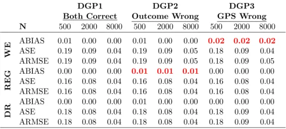
. (3.31) The model specification given in Equation 3.30 is correct for DGP1 and DGP2, but it is wrong for DGP3. Thus, weighting estimators which relies on the estimated GPS based on this model specification will not be consistent for DGP3, but will be consistent for the other DGPs. The outcome model in Equation (3.31) is only correct for DGP1 and DGP3. Hence, the regression estimators will be inconsistent for DGP2. However, the doubly robust estimators which use both model specifications will be consistent for all three DGPs, since for each DGP at least one of the model specifications is correct.

Table 3.3: Summary of Monte Carlo Results

DGP1 DGP2 DGP3

Both Correct Outcome Wrong GPS Wrong N 500 2000 8000 500 2000 8000 500 2000 8000

WE

ABIAS 0.01 0.00 0.00 0.01 0.00 0.00 0.02 0.02 0.02 ASE 0.19 0.09 0.04 0.19 0.09 0.05 0.18 0.09 0.04 ARMSE 0.19 0.09 0.04 0.19 0.09 0.05 0.18 0.09 0.05

R E G ABIAS 0.00 0.00 0.00 0.01 0.01 0.01 0.00 0.00 0.00 ASE 0.16 0.08 0.04 0.16 0.08 0.04 0.16 0.08 0.04 ARMSE 0.16 0.08 0.04 0.16 0.08 0.04 0.16 0.08 0.04

D R ABIAS 0.00 0.00 0.00 0.01 0.00 0.00 0.00 0.00 0.00 ASE 0.18 0.08 0.04 0.18 0.08 0.04 0.18 0.09 0.04 ARMSE 0.18 0.08 0.04 0.18 0.08 0.04 0.18 0.09 0.04 AABIAS: average of absolute bias, ASE: average standard error, ARMSE: aver- age root of the mean squared error over twelve parameter estimates.

The results of the Monte Carlo experiment are summarized in Table 3.3. Here, only the averages of absolute biases (AABIAS), standard errors (ASE) and root of the mean squared errors (ARMSE) over twelve parameters for each DGP are reported.

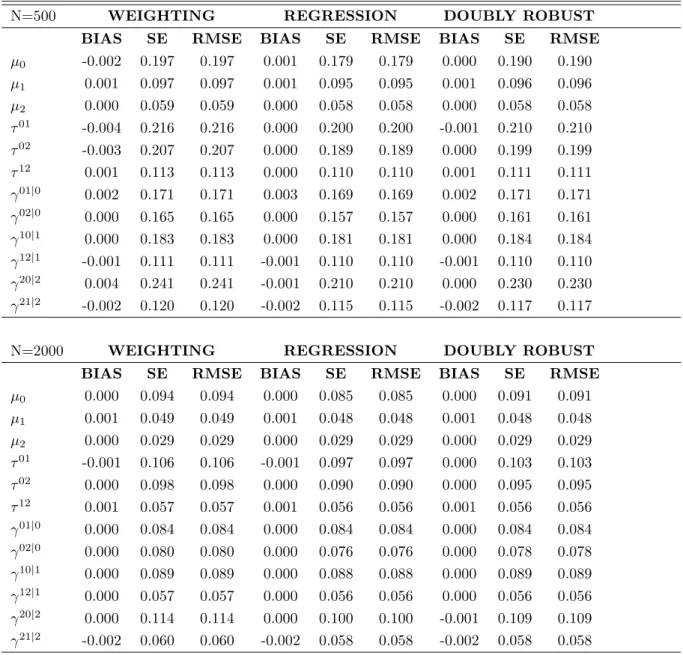
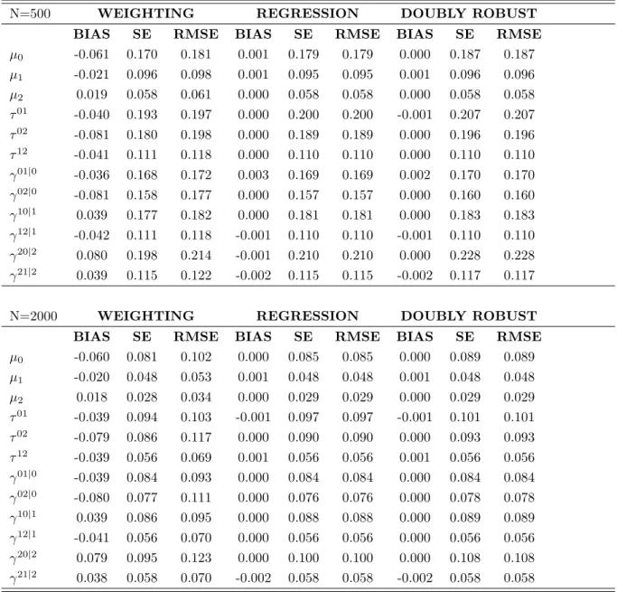
Tables B.1-B.3 display detailed simulation results for each µ

, τ

and γ

. The re- sults clearly demonstrate the double robustness of the proposed estimation method.

Under correct specification of the relevant models, all three methods estimate the

parameters consistently. The most efficient method is the regression method, fol-

lowed by the doubly robust method. The efficiency difference, however, is negligible.

Interestingly, the efficiency of weighting method is only slightly less than the doubly robust method. This might be due to the treatment homogeneity, i.e. treatment effects do not change with the covariates. Under both types of misspecifications, doubly robust estimators stay consistent, whereas the misspecification of the out- come model leads to inconsistent regression estimators and misspecification of the GPS leads to inconsistent weighting estimators, i.e. the biases do not decrease as the sample size increases. Obviously this Monte Carlo study does not consider more general cases like heterogeneous treatment or overlap problems, but it demonstrates the double robustness of the proposed method under misspecification of one of the models. A more comprehensive Monte Carlo study with a more general design is necessary to evaluate the properties of these methods more in detail. This, however, is beyond the scope of this paper.

4 Empirical Study

In the empirical part of this study, the returns to education at different levels are estimated by the doubly robust estimation method explained in Section 2. Estima- tion of causal effects of education on earnings is not trivial. Card (1999) provides a comprehensive review on problems associated with the estimation of the returns to education. The identification of the casual effects requires some strong assumptions on the selection to the participation mechanism either in terms of unobservables or observables. The usual method under assumption of selection on unobservables is the Instrumental Variable (IV) method, where the biggest challenge is to find a valid instrument. Card (1999), Card (2001) review the empirical results based on IV methods. On the other hand, if the assumption of conditional independence, i.e. se- lection on observables, is satisfied, there is no need for an instrumental variable and the causal effects can be identified by controlling for observable characteristics. This assumption however puts strong requirement on the data set. The variables available in a data set should be rich enough such that none of the important confounders of the treatment and outcome variable is left out. Due to data limitations, there are few studies where the causal effects are estimated by methods based on CIA (for example Blundell et al. 2005, Pohlmeier & Pfeiffer 2004, Flossmann & Pohlmeier 2006). The strong data requirement is not a restriction for this study because the data set provides standard control variables like gender, family background etc., as well as variables which are less common in surveys, such as several IQ measures, noncognitive skill measures and behavioral measures. The richness of the control variables makes unobserved ability problem less severe. Moreover, since all the vari- ables are measured during the childhood before the measurement of the wages or any schooling choice is made, the problem of reverse causality is also avoided.

4.1 Data

1970 British Cohort Study (BCS70) is a longitudinal study which includes all the

children born in the UK in the first week of April 1970. Since BCS70 began, there

have been seven full data collection exercises in order to monitor the cohort mem-

bers’ health, education, social and economic circumstances. These took place when

respondents were aged 5, in 1975, aged 10, in 1980, aged 16, in 1986, aged 26, in 1996, aged 30, in 1999-2000, aged 34, in 2004-2005, and aged 38, in 2008-2009. For the empirical study, we use the birth survey, the surveys at the age of 10 and 30.

The birth survey provides background information on the newborn and the parents.

The second sweep, additional to the classical variables, includes very comprehensive measures on noncognitive and cognitive abilities, as well as child’s behavioral prob- lems. The last sweep is used to construct wages and the highest qualification level attained. After dropping all observations with missing information on any of the variables used and removing the children with congenital abnormalities, the sample used consists of 2424 males and 2261 females.

The richness of the measures available in the data set is important for the justifica- tion of the econometric method used in the current study. The crucial assumption is the conditional independence assumption which is not testable; though, it requires having all the important variables which affect both the treatment variable and the outcome variable in the data. Blundell et al. (2005) use another longitudinal study from UK and estimate the returns to schooling using various methods which rely on CIA. They use a rich data set and show some evidence that the assignment to the treatment is unconfounded given pre-treatment variables X. The data set used here contains equivalent information to their data set and some other measures on noncognitive, cognitive ability, as well as child’s behavior. Since the data used here contain comprehensive measures, the CIA is not too unrealistic to hold. Another important issue for the CIA is that the covariates have to be unaffected by the treat- ment. This requirement in our study is fulfilled since the covariates are measured before the minimum school leaving age in the UK.

The outcome variable is the log hourly wages at the time of the fifth sweep. Therefore our sample consists of individuals who were employed at the time of the fifth sweep.

We use the information on the last net payment they received, the period the period that corresponds to the payment and the weekly working hours.

The educational attainment, the treatment variable, is measured in detail in BCS70. For the empirical analysis, the educational attainment is categorized in four groups, which have a sequential nature. Table 4.1 summarizes which qualifications the categories include.

6

In order to construct the outcome variable, as well as the treatment variable, the Appendix by

Bynner et al. (2000) is followed.

Table 4.1: Educational qualifications and mapping to level of qualification

T Level General Vocationally-related Occupational (Academic) (Applied) (Vocational) 0 No qualification No qualification Foundation GNVQ NVQ level 1

GCSE grade D-G Other GNVQ Other NVQ

CSEs grades 2-5 Units towards NVQ

Scottish standard RSA Cert/Other

grades 4-5 Pitmans level 1

Other Scottish Other vocational

school qualification qualifications

HGV 1 O-level GCSE grade A*-C Intermediate GNVQ NVQ level 2

O levels grade A-C BTEC First Certificate Apprenticeships O levels grade D-E BTEC First Diploma City Guilds Part

CSE grade 1 2/Craft/Intermediate

Scottish standard City Guilds Part 1

Other

grades 1-3 RSA First Diploma

Scottish lower Pitmans level 2

or ordinary grades

2 A-Level A level Advanced GNVQ NVQ level 3 AS levels BTEC National Diploma City Guilds Part 3

Scottish Highers ONC/OND Final

Advanced Craft

Scottish Cert of RSA Advanced

Diploma

6th Year Studies Pitmans level 3

3 Higher Education Degree BTEC Higher NVQ level 4-5 HE Diploma Certificate/Diploma Professional degree

Higher Degree HNC/HND qualifications

Nursing/paramedic Other teacher training qualification City Guilds Part 4 Career

Ext/Full Tech RSA Higher Diploma/PGCE

Figure 1 illustrates the distribution of log hourly wages by gender and Figure 2 illustrates the distribution of the wages by education level for males and females separately. Figure 1 does not indicate a big difference in the unconditional wage distribution of females and males. On the other hand, if we look at the wage dis- tributions by educational attainment, we see that the distributions differ for both males and females. As expected, the most observable difference is between higher education and no qualification.

In the second sweep of BCS70, there are several measures related to the child’s

cognitive ability. Three different tests are used to construct indices to measure the

cognitive ability. The first test is called “Friendly Math Test (FMT)”. This test was

developed especially for the use of BCS70. It consists of a total 72 multiple choice questions and covers the rules of arithmetic, numbers skills, fractions, algebra, geom- etry and statistics. The variable is constructed as the number of correctly answered questions.

The second test is the “Shortened Edinburgh Reading Test (SERT) ”. It is the short- ened version of the Edinburgh Reading Test developed by Godfrey Thomson Unit.

The shortened test contains 67 items which examine vocabulary, syntax, sequenc- ing, comprehension and retention. The variable to control for the reading ability is constructed as the sum of the correctly answered questions. The last test is the

“British Ability Scale (BAS)”. This test of cognitive attainment aims at measuring something akin to IQ (Elliot et al. 1978). They are two verbal and two non-verbal subscales. Verbal subscales comprise word definitions (37 items) and word simi- larities (42 items). Non-verbal subscales comprise recall of digits (34 items) and matrices (28 items). For each scale, the variables are constructed as the number of correct answers.

Furthermore, there are two tests related to the noncognitive abilities of the child:

“(Lawseq) Self-Esteem Scale” and “(Caraloc) Locus of Control Scale” available in the second sweep. The Self-Esteem Scale was developed by Lawrence (1973). Lawrence (1973) defines self-esteem as a person’s evaluation of his self-image in relation to his ideal self. The questions used in the survey are listed in the upper part of Table C.1. There are 16 questions, four of which are distractor questions. The distractor questions are marked with a star in the table. Children answer the questions with

“Yes”, “No” or “I do not know”. The index to measure self-esteem is constructed following Lawrence (1996). All “No” answers get two points except for question 1.

For question 1, answering with “Yes” is worth to two points. “I do not know” is worth for one point for all questions. The distractor questions do not contribute to the measure. High scores indicate higher self-esteem. The second noncognitive skill measure is constructed based on the Locus of Control questions. The concept of Locus of Control introduced by Rotter (1966) refers to an individual’s perception about the underlying main causes of the events in his/her life. According to this concept, individuals range between externaliser and internaliser. Externalisers be- lieve that the events in his/her life are caused by external factors like fate or luck.

On the other hand, internalisers believe that the events in his/her life are caused by his/her personal decisions and efforts. The questionnaire was constructed from var- ious tests to measure the locus of control (Gammage 1975). The children are asked 20 questions, to which they answer with “Yes”, “No” or “I do not know”. There are five distractor questions. From the answers a one dimensional scale is constructed as a measure of the degree of internalization. Each “No” response counts as one point, except for the question ten where “Yes” equals one point. The distractor questions do not count for the locus of control index. High scores indicate greater locus of control, i.e. higher degree of internalizing. The questions are listed in Table C.1.

In addition to the above mentioned measures, in the second sweep of BCS70 moth-

ers have completed a set of questions which are related to the behavioral difficulties

of the child. Two different scales are used to construct indices to measure the be- havior disorder. The first one is “Rutter Parental ’A’ Scale of Behavior Disorder”

(Rutter 1967, Rutter et al. 1970) and the second one is “Conner’s Hyperactivity Scale” (Conners 1969). The list of related questions is in Table C.2. For both scales, mothers had to make a vertical mark through the line alongside each statement to indicate to what extent the child shows the behavior described. The line corresponds to a scale from 0 to 100. 0 refers to “does not apply” and 100 refers to “certainly applies”. The overall Rutter score and Connor score for a cohort member at the age of 10 is the sum across the individual variables. Categorical ratings were calcu- lated for each scale by dividing scores into three levels of severity: “normal” scores less than the 80th percentile, “moderate” problem scores between the 80th and 95th percentile and “severe” problem scores above the 95th percentile (this is a simplified version of the technique adopted in a paper by Thompson et al. 2003).

In addition to the cognitive and noncognitive ability measures as well as the behavior disorder measures, some other information on the child’s family background like mother’s age and mother’s education at child’s birth, as well as the ethnicity and the gender of the child from the birth survey are included as controls. The information on household income, total number of children in the household and father’s social class are taken from the second sweep. Furthermore, an indicator variable for whether the child lived with both parents since birth till age of 10 is included. Description of the variables and summary statistics are given in Tables C.3 and C.4, respectively.

4.2 Empirical Results

There are a number of studies dealing with estimation of the returns to schooling. In empirical studies education is usually taken as a binary treatment variable.

Consid- ering multivalued treatment provides the opportunity for a better characterization of the returns to education at different levels. The proposed method described in Section 2, which is doubly robust against misspecification, is used in the econometric analysis. As noted earlier, the advantage of using a doubly robust estimator is that the treatment parameter of interest can be consistently estimated even if one of the underlying methods relies on a misspecified model.

The GPS is estimated by ordered logit, where the dependent variable is different levels of education: no qualification, O-Level, A-Level and higher Education.

The regression results of ordered logit estimation are represented in Table C.5. In Ta- ble C.6, the average partial effects are presented for interested readers. Although

7

The percentiles are calculated using the raw data.

8

Conti et al. 2011 use British Cohort Study in order to estimate the returns to education on non- market outcomes as well as earnings. The study here differs from their study in three important ways. First of all, they use Bayesian econometric methods using factor models. Thus, identification relies on different assumptions. Second, although they provide estimates of returns to education on earnings, the emphasis of their study is non-market outcomes. Furthermore, the education is measured as a dummy variable in their study not as a multivalued treatment variable.

9

For robustness check, the probabilities are also estimated by sequential logit. Treatment effect

estimates do not change qualitatively or quantitatively.

the GPS estimation results are not a direct interest of this study, it is worth men- tioning that the results provide supporting evidence on the importance of cognitive and noncognitive abilities. The Locus of Control Scale, the Shortened Edinburgh Reading Test, the Friendly Math Test as well as some scales of British Ability Test are significant. For both males and females, being internaliser in terms of Locus of Control Scale decreases the probability of having no qualification, whereas increases the probability of having all other degrees. The magnitude of the positive effect is the highest for the O-Level. Higher scores in the Shortened Edinburgh Reading Test and in the Friendly Math Test decrease the probability of having no qualification and increase the probability of having any other degree. For females, similar effects are observable for word similarities scale and word definitions scale of BAS. For males, the word definitions scales and matrices scale of the BAS have significant effects on the probabilities. These results provide further evidence on the effects of cognitive and noncognitive abilities.

In the evaluation literature it is common to inspect the histogram estimates visually to determine lack of overlap. The histogram estimates of the GPS for individuals with T

= t and T

6 = t for each t = { 0, 1, 2, 3 } for male and female samples are plotted in Figures 3 and 4. For females, the boundaries of the histograms have some gaps; however the probabilities over two different groups are distributed over the same interval. For males it seems even less problematic. Thus, there is no need to apply any common support adjustment.

After estimating the weights, the proposed doubly robust estimator is used as ex- plained in Section 2 with corresponding weights to estimate the treatment effect parameters (γ

, τ

, − γ

) as well as the expected earnings for each level of education (µ

). Mean Estimates of the log of earning by education levels are pre- sented in Figure 5. There are significant differences in estimated earnings of females and males for different educational levels. Males earn on average more than females even after controlling for the covariates. For each education level, the expected earn- ings for males are larger than for females.

The estimated treatment effect parameters are summarized in Table 4.2 below. The

results for females and males are reported in the upper and lower part of the table,

respectively. All possible pairwise comparisons for four levels of education are con-

sidered. The reported numbers are % wage gains due to the treatment m relative

to l. Average effect of m relative to l is estimated for three groups: (i) for the

subpopulation T

= m (γ

); (ii) for the entire population (τ

), and (iii) for the

subpopulation T

= l ( − γ

). τ

is estimated as in Equation (2.20) and γ

is

estimated as in Equation (2.23) for all values of m and l. If γ

is higher than τ

and τ

is higher than − γ

, the treatment is “efficient” in terms of the allocation

of individuals to the particular treatment level m, i.e. the individuals who would

benefit at most from the treatment level m are allocated into this treatment. The

difference between γ

and τ

, as well as the difference between τ

and − γ

is called the “sorting gain” (Heckman & Li 2004). For example, if we consider the

return of higher education (m) over no qualification (l), positive sorting gains would

imply that the individuals with higher ability are allocated to the appropriate educa- tional institutions. However, negative sorting gains would indicate that there may be individuals with lower qualifications who should have received a higher educational degree according to their abilities.

Table 4.2: Estimated Treatment Parameters: Average effect of m relative to l

m l ˆ γ

τ ˆ

− ˆ γ

F e m a le s

Higher Education No Qualification 19.0*** 18.8*** 16.8***

Higher Education O-Level 20.7*** 19.2*** 18.4***

Higher Education A-Level 14.0*** 15.1*** 17.5***

A-Level No Qualification 2.9 3.7 2.4

A-Level O-Level 2.9 4.2 2.6

O-Level No Qualification 0.4 -0.5 1.4

m l ˆ γ

τ ˆ

− ˆ γ

M a le s

Higher Education No Qualification 18.5*** 22.1*** 23.3***

Higher Education O-Level 13.3*** 16.8*** 18.3***

Higher Education A-Level 11.9*** 14.1*** 15.3***

A-Level No Qualification 9.4*** 8.0*** 7.2***

A-Level O-Level 3.5 2.7 2.8

O-Level No Qualification 5.7** 5.3* 3.4

Note : % wage gains due to the treatment are reported. *** 1% significance level, ** 5% significance level, * 10% significance level. Standard errors are calculated based on the asymptotic variance.

Females who have received higher education earn on average 19 % more by get- ting higher education instead of no qualification. The wage gain due to higher education compared to no qualification for the entire female sample is 18.8%. On the other hand, the percentage wage gain due to higher education for females who do not have any qualifications would be 16.8. Although, the differences between treatment effect estimates are very small, positive sorting gains are observed for females when returns to higher education is compared to no qualification. If we compare the corresponding results for males (18.5%, 22.1%, 23.3%), the ascending order (γ

< τ

< − γ

)of the percentage wage gains indicate negative sorting gains. Males without any qualification would earn 23.3% more if they had received higher education, whereas those with a higher education degree earn only 18.5%

more due to the higher education. This implies that the selection of males into higher education is “inefficient“. Similarly, when higher education is compared with O-level, positive sorting gains are observed for females (20.7%, 19.2%, 18.4%) but negative for males (13.3%, 16.8%, 18.3%). This situation changes for females if the returns of higher education versus A-Level is compared: here the sorting gains are negative for both females (14%, 15.1%, 17.5%) and males (11.9%, 14.1%, 15.3%).

Other pairwise comparisons for females do not yield any significant results. For males, significant gains due to A-Level over no qualification with positive sorting (9.4%, 8.0%, 7.2%) are observed. The gain over O-level over no qualification is also significant for males whose highest qualification is O-Level. The overall percentage wage gain due to O-level over no qualification is 5.3% but it is only significant at

10

Flossmann & Pohlmeier (2006) use the same argument to when comparing the average causal

returns for the German school tracks.

10% significance level.

Another striking result is that the percentage wage gain due to higher education versus any other lower educational attainment is higher for highly educated females than highly educated males. The difference is highest for higher education versus O-level. The percentage gain due to the higher education over O-level is 20.7% for highly educated females, whereas the same pairwise comparison for the males who received higher education suggests only 13.3% wage gain. On the other hand, males who have lower educational attainments like A-Level and O-Level benefit more from these attainments than females when compared to no qualification. If we consider the average returns of different levels of education for the entire population by gender, we see that the returns to higher education over no qualification are higher for males (22.1%) than for females (18.8%). However, the expected effect of higher education compared to O-level and A-level is higher for females (19.2%, 15.1%) than for males (16.6%, 14.1%).

5 Conclusion

In this paper, the returns to different levels of education are estimated using a novel estimation method. The proposed method is an extension of the doubly robust ATE and TT estimator in binary treatment case to the multivalued treatment evalua- tion problem under CIA. It combines the regression adjustment approach with the weighting approach. Regression adjustment requires model specifications for the con- ditional mean functions and the weighting approach requires model specification for the generalized propensity score. The advantage of the combination of the two meth- ods is that the doubly robust method estimates the treatment parameter of interest consistently even if one of the models is misspecified. The estimation procedure is defined explicitly and the asymptotic distribution of the parameters is derived. The results generalize the studies by Hirano & Imbens (2001) and Wooldridge (2007) for multivalued treatment variables. Furthermore, a small Monte Carlo experiment is used to demonstrate the double robustness property of the proposed estimation method. The results clearly indicate that even if only one of the underlying models is correctly specified, the proposed method gives consistent estimates of the treat- ment parameters. Under correct specification of the outcome model, the regression adjustment is the most efficient one, but the efficiency difference between regres- sion and doubly robust method is slight. These results indicate that the use of the doubly robust methods to estimate treatment parameters in multivalued treatment evaluation provide protection against misspecification at almost no efficiency costs.

Given that in an empirical study it is difficult to be sure about the correctness of the

model, doubly robust methods provides more chances to hit the correct model with

no significant costs. Furthermore, the generalization introduced here is applicable

to a wide range of program evaluation questions, since it deals with multivalued

treatment effect. Given that the method is just a weighted regression; any standard

econometric method can be used in practice.

In the empirical part of this paper, the unique data set of the British Cohort Study is

used. Availability of various measures for cognitive and noncognitive ability as well

as for behavioral disorder beyond the standard covariates makes CIA more likely to

be valid. The effects are analyzed separately for males and females. The estimated

earnings of females and males for different educational levels are found to be signifi-

cantly different. The expected earnings for males are larger than that of females for

any education level. The estimated treatment effects of different educational levels

are also shown to be different for males and females. The percentage wage gains

due to the higher education, A-Level and O-level over no qualification are higher

for males than females if the entire population is considered. However, females’ per-

centage wage gains due to the higher education over A-Level and O-Level are higher

than males’ gains. The results also suggest that highly educated women gain more

from higher education than highly educated men on average.

References

Bang, H. & Robins, J. M. (2005), ‘Doubly robust estimation in missing data and causal inference models’, Biometrics 61(4), 962–973.

Blanden, J., Gregg, P. & Macmillan, L. (2007), ‘Accounting for intergenerational income persistence: Noncognitive skills, ability and education*’, The Economic Journal 117(519), C43–C60.

Blundell, R., Dearden, L. & Sianesi, B. (2005), ‘Evaluating the effect of education on earnings: models, methods and results from the National Child Development Survey’, Journal of the Royal Statistical Society. Series A (Statistics in Society) 168(3), 473–512.

Bynner, J., Butler, N., Ferri, E., Shepherd, P. & Smith, K. (2000), The design and conduct of the 1999-2000 surveys of the National Child Development Study and the 1970 British Cohort Study, CLS Cohort Studies Working Paper 1, Centre for Longitudinal Studies, Institute of Education University of London.

Card, D. (1999), Chapter 30 the causal effect of education on earnings, in O. C.

Ashenfelter & D. Card, eds, ‘Handbook of Labor Economics’, Vol. 3, Part A of Handbook of Labor Economics, Elsevier, pp. 1801 – 1863.

Card, D. (2001), ‘Estimating the return to schooling: Progress on some persistent econometric problems’, Econometrica 69(5), 1127–1160.

Carneiro, P., Crawford, C. & Goodman, A. (2007), Which skills matter?, in D. Ke- hoe, ed., ‘Practice Makes Perfect: The Importance of Practical Learning’, Social Markets Foundation, London, pp. 22–38.

Cattaneo, M. D. (2010), ‘Efficient semiparametric estimation of multi-valued treat- ment effects under ignorability’, Journal of Econometrics 155(2), 138 – 154.

Conners, C. K. (1969), ‘A teacher rating scale for use in drug studies with children’, American Journal of Psychiatry 126, 884–888.

Conti, G., Heckman, J. J., Lopes, H. F. & Piatek, R. (2011), Constructing econom- ically justified aggregates: An application of the early origins of health, Working paper, Department of Economics, University of Chicago.

Elliot, C., Murray, D. J. & Pearson, J. (1978), British ability scales; manual 3: Direc-

tions for administration and scoring and manual 4: Tables of abilities and norms,