Geological Processes
I -D
zur
Erlangung des Doktorgrades
der Mathematisch-Naturwissenschaftlichen Fakultät der Universität zu Köln
vorgelegt von Johannes Stefanski
aus Weimar
Köln, 2020
INSTITUT FÜR GEOLOGIE UND MINERALOGIE
Öffentliche Verteidigung: 26.09.2019, Universität zu Köln, Institut für Geologie und Miner- alogie, Zülpicher Strasse 49b
Promotionskommission: Prof. Dr. Georg Bareth, Universität Köln (Vorsitzender)
Prof. Dr. Sandro Jahn, Universität Köln (Erstgutachter)
Prof. Dr. Thomas Wagner, RWTH Aachen (Zweitgutachter)
ACKNOWLEDGEMENTS
I wish to express my gratitude to Prof. Dr. Sandro Jahn for the supervision of my PhD project.
In particular, for the support in scientific paper writing as well as the preparation of conference presentations and the inspiring discussions over the last years. I want to especially thank Dr.
Clemens Prescher for his patient training in the performance of high pressure experiments and data analysis. Furthermore, also Dr. Christian Schmidt who helped me in the beginning of my PhD to construct a hydrothermal diamond anvil cell and showed me how to perform experiments with this device. Just as well Gunther Pillunat for his collaboration in planning and in constructing the in house diamond anvil cell heating system. I would also like to thank Dr. Sergio Speziale for the support and help to carry out high pressure experiments in combination with Brillouin spectroscopy in a side project of my PhD study. For helpful discussions regarding solute complexation and aqueous geochemical modeling I want to thank Prof Dr. Thomas Wagner. Moreover, I also want to thank Prof Dr. Ladislav Bohat˝ for providing BeO samples for experiments in the first year of my PhD.
I owe a great debt of gratitude to the Deutsche Forschungsgesellschaft that financed parts of this PhD work in the framework of the project: JA 1469/10-1, as well as the Gauss Centre for Supercomputing e.V. for funding this thesis by providing computing time through the John von Neumann Institute for Computing (NIC) on the Supercomputer JUQUEEN, JURECA and JUWELS at Jülich Supercomputing Centre (JSC).
I wish to thank Ivonne Gebhard for her great support during the last years as well as my
parents Christina Stefanski and Dr. Reiner Stefanski for many years of unrestricted support
over my bumpy course of education. Furthermore, Laura Ritterbach and Linda Kerkhoff for
their kind office collaboration. Last but not least I want to thank all colleagues for the pleasant
working atmosphere during my time in Cologne.
ZUSAMMENFASSUNG
Wässrige geologische Fluide treten in allen Bereichen unseres Planeten und anderen ter- restrischen Körpern auf. Sie spielen nicht nur eine wichtige Rolle bei der Entstehung des Lebens, sondern auch bei Prozessen in der Erdkruste und des Erdmantels, z.B. bei der Metaso- matose. Die Verbindung von makroskopischen Besonderheiten von Materialien der Erde mit den Eigenschaften auf der molekularen Skala war jeher ein zentrales Anliegen der Mineralogie und Petrologie. Dennoch ist die Beschreibung von strukturellen und thermodynamischen Eigen- schaften dieser Fluide bis heute nicht voll erfasst. Experimentelle Studien mittels hydrother- maler Autoklaven, Druckbehälter oder hydrothermaler Diamantstempelzellen in Verbindung mit spektroskopischen und potentiometrischen Untersuchungen sind limitiert in ihrem Temperatur-, Druck- und chemischen Zusammensetzungsbereich. Seit dem Ende des letzten Jahrtausends sind Molekulardynamik Computersimulationen ein fester Bestandteil der Untersuchungen von wässrigen Lösungen auf der molekularen Skala. Mit Beginn dieses Jahrhunderts ist es, dank weitreichender Entwicklungen in der Computertechnologie, sogar möglich, ab initio Moleku- lardynamik Simulationen durchzuführen. Diese liefern neue Einblicke in die Gesteins-Fluid Wechselwirkung und außerdem wichtige Beiträge für das Verständnis von experimentellen Ergebnissen.
In dieser Arbeit wurden drei aquatische geochemische Systeme mittels ab initio Molekular- dynamik in Verbindung mit neuesten Methoden zur Untersuchung des Konfigurationsraumes studiert. In der ersten Fallstudie wurde die Assoziation von Yttrium, als ein Vertreter der Gruppe der schweren Seltenen-Erdelemente, mit Chlor und Fluor untersucht. Es konnte nicht nur gezeigt werden, dass Yttrium-Fluor Komplexe stabiler sind als Yttrium-Chlor Komplexe.
Vielmehr sollten schon geringe Fluoraktivitäten im Fluid ausreichen, um diese zu bilden.
Darüber hinaus wurde entdeckt, dass die Protolyse von Wassermolekülen in der Umgebung des Yttrium-Ions unter extremen Druck- und Temperaturbedingungen ansteigt. Diese Beobachtung scheint übertragbar auch auf andere sogenannte „high field strength elements“ zu sein.
In der zweiten Fallstudie wurde das Verhalten von Beryllium in konzentrierten fluorreichen
hydrothermalen Fluiden untersucht. Dabei zeigte sich, dass Beryllium zu einer trigonalen
Koordination unter hydrothermalen Hochtemperatur-Bedingungen tendiert, im Gegensatz zu der
stabilen tetraedrischen Koordination unter Raumbedingungen. Diese Beobachtung deutet auf eine höhere Mobilität von Beryllium in hydrothermalen Lösungen hin, als bisher angenommen wurde. Des Weiteren konnte eine Inkonsistenz der tabellarisierten thermodynamischen Daten von aquatischen Beryllium-Fluor Komplexen in der weitverbreiteten „slop89.dat“ Datenbank entdeckt werden.
In der letzten Fallstudie dieser Arbeit wurden die Änderungen der Hydratation des Fluorid- Ions und der Flusssäure mit steigender Temperatur und Kompression untersucht. Es ist dies die erste Studie zu den molekularen Eigenschaften von Fluor-Speziationen in wässrigen Fluiden unter Druck- und Temperaturbedingen der Erdkruste und des oberen Erdmantels. Sie liefert damit wichtige Informationen über die Wechselwirkung des Halogens mit dem Lösungsmittel.
Darüber hinaus konnte die Säurekonstante von Flusssäure in dem untersuchten Bedingungs- bereich bestimmt werden. Die Resultate könnten wichtige Erkenntnisse für die Rolle des Fluor bei der Mobilisierung und dem Transport von Metallionen in hydrothermaler Lösung unter extremen Druck liefern.
Es hat sich aber auch gezeigt, dass noch mehr Erfahrung und neue Konzepte für die
Verbindung von klassischen thermodynamischen Datensätzen und atomarer Computersimu-
lation nötig sind.
ABSTRACT
Aqueous geological fluids occur on the surface and in great depth on our planet and other terrestrial bodies. They play an important role in the origin of life, and further in processes of the Earth’s crust like the genesis of economically significant ore deposits and metasomatism down to the Earth’s mantle. The relations between the molecular scale and macroscopic properties of earth materials is in the focus of mineralogy and petrology. But the development of structural and thermodynamic models of geological fluids are still a great challenge today.
Experimental studies at high temperature and high pressure use devices like hydrothermal autoclaves, pressure vessels or heated/hydrothermal diamond anvil cells in combination with spectroscopic or potentiometric measurements that are limited in pressure, temperature and composition range.
Since the end of the last millennium, molecular dynamics have become an important tool to investigate not only molecular structural changes of solvents, but also thermophysical properties of solutes in geological fluid were investigated on a molecular scale. In the current century thanks to computer technology revolutions ab initio molecular dynamics simulations provide new insight into rock-fluid interaction processes and support the interpretations of experimental results.
In this thesis, three different aqueous geochemistry systems are investigated using ab initio
molecular dynamics in conjunction with advanced free energy sampling methods. Firstly,
the free energy of yttrium-halide (F fluorine, Cl chlorine) aqueous complexes formation were
probed by constrained ab initio molecular dynamics. In this case study it was found that
yttrium drives the self-ionization in vicinal water molecules. Further stable Y-Cl/F complexes
are found and there thermodynamic stabilities can be reported. This results have revealed
that yttrium builds more stable complexes with fluorine than with chlorine. Therefore, very
low F activity enables the formation of Y-fluorine complexes. Secondly, the behavior of
beryllium in fluorine rich hydrothermal fluid was investigated. It was shown that beryllium
tends to form a trigonal coordination at high temperature conditions in comparison to tetrahedral
coordination at ambient conditions. That change might cause a higher solubility of beryllium in
hydrothermal brines as known from its geochemical relative zinc. Furthermore, in this case study
inconsistencies of the widely used thermodynamic database slop98.dat regarding to aqueous beryllium complexes are discovered. In the last case study, new insight into the behavior of fluorine and hydrofluoric acid in aqueous solution with increasing temperature and compression were gained. Moreover, acidity constants of hydrofluoric acid using novel sampling methods were derived. This thermodynamic data might lead to a better understanding of the role of fluorine for the transport of metal ions in geological fluids under very high pressures.
The ab initio simulations presented in this thesis do not only provide a detailed insight into
the molecular structures of matter, apart from that they enabled the access of thermodynamic
properties such as species stability constants or acidity constants. But more experience and
new correlation models are necessary to combine results of this simulation with ordinary
derived thermodynamic properties of electrolytes and non-electrolytes at elevated temperature
and pressure conditions.
TABLE OF CONTENTS
Acknowledgements . . . iii
Abstract . . . vi
Table of Contents . . . viii
List of Illustrations . . . ix
List of Tables . . . xii
Nomenclature . . . xiii
Thesis Organization . . . . 1
Chapter I: General Introduction . . . . 2
1.1 Geological Aqueous Fluids . . . . 2
1.2 Basic Properties of Geological Aqueous Fluids . . . . 6
1.3 Aim of this Theses . . . . 9
Published Content and Contributions . . . 10
Chapter II: Methods . . . 11
2.1 Thermodynamic Approaches . . . 11
2.2 Ab Initio Molecular Dynamics . . . 18
2.3 Analysis of Interaction Distances and Coordination Numbers . . . 23
2.4 Free Energy Sampling Methods . . . 25
Chapter III: Case Study I: Yttrium Speciation in Subduction Zone Fluids . . . 29
3.1 Computation and Thermodynamic Approach . . . 32
3.2 Results . . . 35
3.3 Discussion . . . 51
3.4 Summary and Conclusion . . . 60
Chapter IV: Case Study II: Beryllium-Fluoride Complexation in Hydrothermal and Late Magmatic Fluids from First Principles Molecular Dynamics . . . 62
4.1 Computation and Thermodynamic Approach . . . 64
4.2 Results and Discussion . . . 67
4.3 Conclusion . . . 78
Chapter V: Case Study III: Formation of Hydrofluoric Acid in Aqueous Solutions under High Temperature and High Pressure . . . 81
5.1 Computation and Thermodynamic Approach . . . 83
5.2 Results . . . 88
5.3 Discussion . . . 99
5.4 Conclusion . . . 105
Chapter VI: Discussion and Outlook . . . 107
Bibliography . . . 111
Appendix . . . 149
Erklärung der Eigenständigkeit . . . 161
LIST OF ILLUSTRATIONS
Number Page
1.1 P / T water phase diagram . . . . 7 1.2 Comparison of the equations of state by Wagner and Pruß [2002], Zhang and Duan
[2005], Mantegazzi et al. [2013] of pure water in a pressure vs. density diagram . . 9 2.1 Illustration of periodic boundary conditions in two dimensions applied in molecular
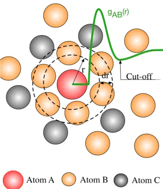
dynamics . . . 22 2.2 Illustration of the radial distribution function in two dimensions . . . 24 3.1 Case study I: snapshot of a simulation cell containing a [ YCl
3( H
2O )
4]
aqcomplex
and 3 NaCl units . . . 33 3.2 (I) potential of mean force of the dissociation reaction of YCl
3to YCl
+2at 1.3 GPa and
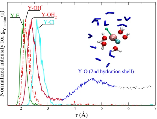
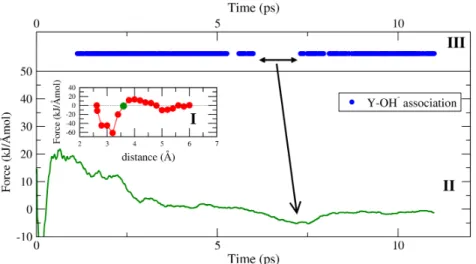
800 C over a distance between 2.63 Å and 6.0 Å. The evolution of the Helmholtz free energy is shown in (II). (A-D) indicate the different stages of the dissociation of the initial complex (see text for details). (III) shows exemplary the progress of the constraint force with simulation time for stage B for a Y-Cl distance of 3.0 Å. . . 34 3.3 Case study I: radial distribution functions of Y-(Cl,O,F) to illustrate its relation to
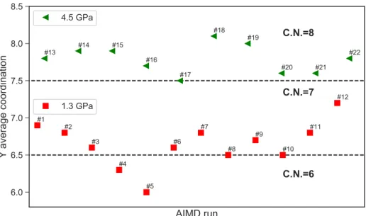
the atomic structure of the aqueous species . . . 39 3.4 Case study I: average yttrium coordination by chloride, fluoride and oxygen at
800 C and 1.3/4.5 GPa . . . 40 3.5 Case study I: appearance of selected ion pairs or complexes during the different
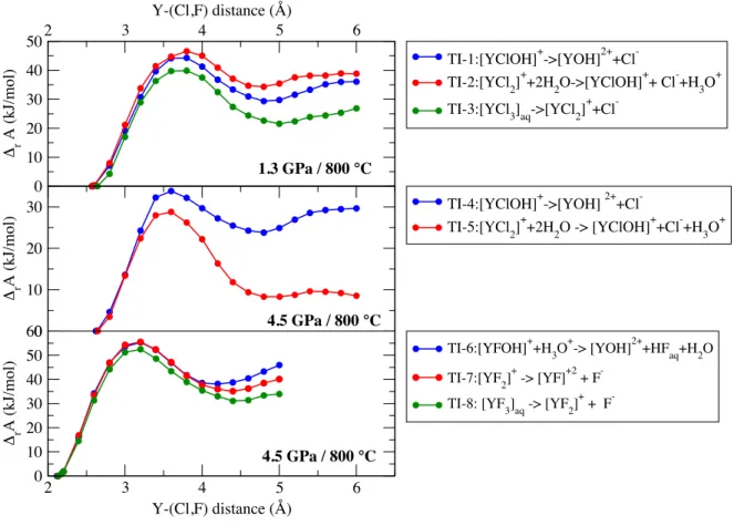
AIMD simulations . . . 41 3.6 Case study I: hydroxide formation within the first hydration shell of the yttrium ion 43 3.7 Case study I: effect of the hydroxide formation on the potential of mean force . . . 47 3.8 Case study I: evolution of the Helmholtz free energy derived from thermodynamic
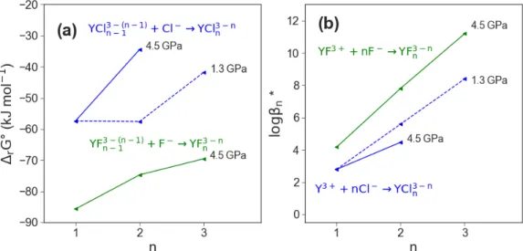
integration for Y-Cl/F complexes at 800 C and 1.3/4.5 GPa . . . 49 3.9 Case study I: the reaction Gibbs free energy
rG of the different formation reactions
and the change of the logarithmic stability constant . . . 50
3.10 Case study I: comparison of the average yttrium hydroxide coordination number between the different complexes . . . 52 3.11 Case study I: comparison of the aqueous species stability derived from the AIMD
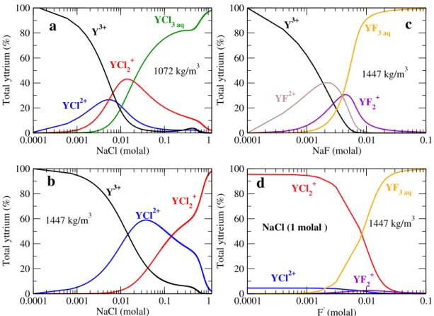
simulation and HKF regression . . . 56 3.12 Case study I: yttrium chloride and fluoride species distribution . . . 58 4.1 Case study II: snapshot of a simulation cell carrying one beryllium ion and four
fluorides with the evolution of the constraint force between the beryllium ion and one of the fluorids . . . 66 4.2 Case study II: snapshot of the formed aqueous beryllium-fluroide complexes . . . . 68 4.3 Case study II: coordination number of beryllium in respect to oxygen and fluoride
in the first hydration shell over the investigated pressure and temperature range . . . 70 4.4 Case study II: radial distribution function between beryllium and oxygen at room
temperature and 727 C . . . 71 4.5 Case study II: potential of mean force between beryllium and fluoride . . . 73 4.6 Case study II: evolution of the Helmholtz free energy difference as a function of the
beryllium-fluoride atomic distance of different aqueous dissociation reactions . . . 75 4.7 Case study II: plot of the logarithmic stability constants of beryllium-fluoride aque-
ous complexes . . . 79 5.1 Case study III: the switch function that is used to define the collective variable
during the well-tempered metadynamics simulation and an exemplary evolution of the collective variable over time at high temperature . . . 87 5.2 Case study III: the radial distribution function between fluoride and hydrogen for
diffrent system pressures . . . 88 5.3 Case study III: the change of the intra- and intermolecular coordination of fluoride
and hydrofluoric acid as a function of pressure . . . 89 5.4 Case study III: evolution of the atomic distances between fluroine, hydrogen and
oxygen as a function of pressure . . . 90 5.5 Case study III: two snapshots of the simulation cell containing one hydrofluoric
acid molecule . . . 91
5.6 Case study III: evolution of the intra- and intermolecular coordination of fluorine species as a function of time . . . 91 5.7 Case study III: free energy surface of the dissociation reaction of hydrofluoric acid
derived from well-tempered metadynamics and the time evolution of the corre- sponding free energy change . . . 93 5.8 Case study III: an example of the evolution of a collective variable over time with
the height of the added Gaussian in the well-tempered metadynamics . . . 96 5.9 Case study III: change of the fluoride and hydrofluoric acid coordination during the
well-tempered metadynamics runs as function of pressure . . . 97 5.10 Case study III: potential of mean force and Helmholtz reaction free energy of a
hydrofluoric acid dissociation reaction at 327 C and 18 MPa . . . 98 5.11 Case study III: variation in the computed Helmholtz reaction free energy and in the
acidity constant of hydrofluoric acid as a function of the logarithmic water density in comparison with experimental results and theoretical predictions . . . 99 5.12 Case study III: change of the acidity constant of hydrofluoric acid along the water
vapor curve . . . 102 5.13 Case study III: relation between the hydration number of halogen species in low
density supercritical fluids, the ionic radius and the logarithm of the fuid/melt
partition coefficient of the halogen ions by Bureau et al. [2000] . . . 104
LIST OF TABLES
Number Page
3.1 Case study I: number of atoms in the different simulation cells together with the size of the cells and the system densities . . . 33 3.2 Case study I: list of atomic distances, coordination numbers and the lifetime of the
initial atomic configuration . . . 37 3.3 Case study I: list of the simulation runs with their initial coordination complexes
and complexes observed for at least 3 ps during the simulation . . . 38 3.4 Case study I: list of the formation Gibbs free energies derived from ab initio
thermodynamic integration . . . 46 3.5 Case study I: list of the logarithmic stability constants derived from ab initio ther-
modynamic integration in comparison to theoretical predication . . . 50 4.1 Case study II: simulation parameters . . . 65 4.2 Case study II: geometrical properties of the investigated beryllium-fluoride aqueous
complexes . . . 69 4.3 Case study II: results of the thermodynamic integration . . . 76 4.4 Case study II: list of the logarithmic stability constants of beryllium-fluoride aqueous
species . . . 77 4.5 Case study II: parameters of the modified Ryzhenko–Bryzgalin model in the
beryllium-fluoride system . . . 78 5.1 Case study III: densities of the simulation cell at 727 C and 327 C . . . 85 5.2 Case study III: list of atomic distances and coordination numbers averaged over the
simulation time . . . 92 5.3 Case study III: list of the well-tempered metadynamics simulation conditions and
the computed reaction Helmholtz free energies, acidity constants and the observed coordination numbers of fluoride and hydrofluoric acid in respect to H
2O and H
3O 94 5.4 Case study III: density model parameter derived from the well-tempered metady-
namics simulations for the dissocation of hydrofluoric acid at 327 C . . . 101
NOMENCLATURE
Acronyms
ab initio general meaning from the beginning, in context of this thesis: all calculation only based on fundamental natural constants
AIMD ab initio molecular dynamics CV collective variable
CN coordination number
DB Debye-Hückel
FES free energy surface
HKF Helgeson-Kirkham-Flowers (model)
IAPWS International Association for the Properties of Water and Steam
L ligand
MD (classic) molecular dynamics metaD metadynamics
M metal ion
ML
nmetal complex with n ligands MOR mid-oceanic ridge
MORB mid-oceanic ridge basalt PP pseudopotentials
ps picosecond
RB Ryzhenko–Bryzgalin (model) REE rare earth elements
TI thermodynamic integration UHP ultra high pressure
USGS United States Geological Survey WTmetaD well-tempered metadynamics XC exchange-correlation functional
Fundamental physical constants
k
BBoltzmann constant (1.38065 · 10
-23m
2kg / s
2K)
N
aAvogardo constant (6.0221 · 10
23mol
1)
R ideal gas constant (molar gas constant) (8.31446 J/K mol)
Superscripts
refers to the standard or reference state
⇤
refers to stability constant that involves further transition states
Subscripts
aq dissolved in aqueous solution
g gas
H
2O properties refer to pure water i any specified species or component sat saturated water pressure
s solid
r refers to a reaction
THESIS ORGANIZATION
This thesis is divided into four main parts. The first part includes a general introduction to the
topic and the methodology in chapter 1 and 2. It is followed by the main part that is constructed
of three case studies of different aqueous geochemistry systems. For every case, the subject
of the study is outlined in context of current scientific knowledge, its aim and case specific
methods and approaches are described in chapters 3,4 and 5. Moreover, for each study results
and possible implications are discussed. In the third part, the reader finds an overall discussion
and conclusion with a outlook for further studies building upon this thesis. The last part includes
the bibliography and an appendix with computing codes of the thermodynamic modeling that
were used and a declaration of originality.
C h a p t e r 1
GENERAL INTRODUCTION
1.1 Geological Aqueous Fluids
Geological aqueous fluids are key agents in many geological processes ranging from the surface to the deep interior of the Earth and other terrestrial plants [Harlov and Aranovich, 2018].
Their interaction with minerals and rocks results in alterations including the dissolution and precipitation of minerals and/or the exchange of chemical elements and isotopes. Fluid-mediated elements and energy transport are important processes, e.g. of deep element cycles in subduction zones (for more detail see Manning [2004], Manning et al. [2013], Keppler [2017]) or during the formation of magmatic-hydrothermal ore deposits (e.g see Hedenquist and Lowenstern [1994], Ridley [2013]). In geochemistry, aqueous phases are commonly distinguished according to their state of matter as liquids or rather aqueous solutions, vapors and supercritical fluids. This distinction does depend on the pressure (P) and temperature (T ) of the geological environment where these phases occur [Pokrovski et al., 2013]. These phases are never pure substances, they contain a variety of elements. But the main solvent is H
2O in the Earth’s crust, upper-mantle and even in the lower-mantle as recent discoveries by Tschauner et al. [2018] of water in diamond inclusions indicate. Moreover, there are numerous evidences that at least for deep fluids carbon (CO
2) can be a main component or even the dominate solvent [Manning et al., 2013].
Our knowledge about these phases derives from a variety of observations in nature: on the one hand, from direct probing of released solutions [Foustoukos and Seyfried, 2007] in geothermal systems, e.g. in hot springs on the continents or in black and white smokers on the mid-ocean ridge (MOR) and the sea floor. Here, meteoric water and seawater migrates 4-8 km deep and is heated up to temperatures of ⇠ 400 C and returns density driven to the surface [Klein et al., 1977, Bibby et al., 1995, Arnórsson et al., 2007]. On the other site, there are fluid inclusions, primary hosted in ore forming or pegmatitic related rocks [Seward et al., 2014] but also in low and high grade metamorphic rocks [Touret, 1977, Ferrando et al., 2005].
They are fundamental information carriers for geologist and mineralogists. The methodology
to investigate the origin, physical properties and composition of this microscopic inclusions (for an overview see Van den Kerkhof and Hein [2001]) was developed and improved over the last decades, since the first scientific description of a fluid inclusion by Sorby [1858].
Furthermore, experiments like in-situ UV-Vis [Wincott and Vaughan, 2006], X-ray absorption spectroscopy [Sanchez-Valle, 2013] and numerical modeling based on thermodynamic data e.g. [Barnes et al., 1966, Sverjensky, 1987, Shock and Helgeson, 1988, Sverjensky, 2019] are essential tools to study processes and properties of such solutions. But there are still many open questions in terms of the chemistry and transport properties of geological fluids. Besides the lack of thermodynamic and speciation data for complex fluids at high temperature and high pressure, existing thermodynamic models have clear limitations [Dolejö, 2013, Seward et al., 2014]. While further experimental efforts are indispensable for providing missing information, molecular dynamics (MD) and ab initio molecular dynamics (AIMD) simulations have become a powerful alternative approach to study the structure and thermodynamics of aqueous fluids [Driesner, 2013, Sherman, 2010] .
Aqueous Fluid in Metasomatic Processes
In subduction zones where oceanic and continental material is transported into the Earth’s mantle, a geotherm evolves that is characterized by rapid increase in pressure, but less in temperature in comparison to the oceanic or continental geotherm (see Fig. 1.1 and for more details Winter [2009] chapter 16). During the subduction process, water rich minerals such as amphibole, serpentine, lawsonite, phengite and other hydrous solid phases [Schmidt and Poli, 1998, Ulmer and Trommsdorff, 1995, Crawford and Fyfe, 1965, Domanik and Holloway, 1996, Zheng et al., 2016, Wunder, 1998] become unstable and release water into the system.
Furthermore, partial melting of crustal or mantle rocks leads to the release of high density aqueous phases in the subducted slabs [Zheng et al., 2011]. But there are more sources of geological aqueous fluids. As has been pointed out, sea and meteoric surface waters have the ability to serve as H
2sources in deep crustal hydrothermal systems [Yardley and Bodnar, 2014].
Therefore, they undergo a downward penetration or upward infiltration after being transported
as pore fluid into the subduction process. But it is generally accepted that this kind of water
source is not the main source for deeper processes in the Eath’s crust or mantle due to the
decreasing amount of porosity with proceeding diagenesis. It is expected, that only one third
of the initially subducted water reaches the subarc and postarc depths and enters the Earth’s mantle [Hacker, 2008].
The knowledge of the composition of subduction zone fluids is primarily derived from chemical analysis of island-arc basalt [Manning, 2004, Métrich and Wallace, 2008] and veins in ultra-high-pressure (UHP) metamorphic rocks (e.g. Svensen et al. [2008], Zhang et al.
[2008], John et al. [2011]). Deep aqueous fluids are mixtures of different ingredients: H
2O, gases (mainly CO
2) , salts and host rock oxide components like SiO
2, Al
2O
3etc. [Manning, 2018]. Field observations of rare halite minerals, fluid inclusions, and high chlorine content of UHP minerals are interpreted as evidence that these fluids are brines [Trommsdorff et al., 1985, Touret, 1977, Newton et al., 1998, Markl and Bucher, 1998]. Because of changes in electrical conductivity with depth in subducted oceanic crust, it is assumed that there is a salinity range between 0.2 and 7.0 wt% [Bucher and Stober, 2010, Sakuma and Ichiki, 2016, Sinmyo and Keppler, 2016] but even higher concentrations are realistic [Métrich and Wallace, 2008, Manning, 2018].
The dissolution of chlorine, fluorine and other anions dramatically increases the solubility potential of minerals at high pressures and high temperatures [Manning and Aranovich, 2014].
The reasons for that are discussed in section 2.1. In general, the presence of a hydrous phase in a metamorphic system has dramatic impact on the mineral formation. Not only that the stability field of UHP minerals changes dramatically as shown in numerous experiments (reviewed by Kawamoto [2006], Ohtani and Litasov [2006], Beran and Libowitzky [2006]), it leads to a fast kinetics of mineral reactions and enables a large-scale mineral replacement on a rather short time scale [Putnis and John, 2010]. Furthermore, a massive increase in the mobility of trace-elements is reported in a variety of field studies [Ayers, 1998, Scambelluri and Philippot, 2001, Kamber et al., 2002, Harlov et al., 2006]. Therefore, a subduction zone fluid can change the geochemical signatures of petrological processes [Winter, 2009, John et al., 2011, Manning, 2004, Keppler, 2017].
Ore deposits are geochemical anomalies, because one or more elements are significantly
enriched in comparison to the Earth’s crustal average. These sites on our planet are particularly
important for humanity, because they are an industrial source of metals as for instance Cu, Au,
Zn, REE, Be etc. for technological application. In hydrothermal ore deposits, ore minerals are precipitated from a high temperature aqueous phase. Those deposits are formed associated with small clusters of magmatic dykes or large intrusion bodies as for example rare earth element deposits [Chakhmouradian and Zaitsev, 2012, Kynicky et al., 2012, Williams-Jones et al., 2000]. In general, those intrusion bodies are formed by melts that segregate from large plutons and migrate upwards in the crust a few kilometers below the surface. The main heat source of these hydrothermal solutions is the magmatic crystallization process [Shmulovich et al., 1995], whereas the water sources of hydrothermal fluids are very diverse. One source is the decomposition of an immiscible aqueous phase from a highly fractionated melt in the late stage of igneous rock formation [Winter, 2009, Philpotts and Ague, 2009]. Here, volatile components (H
2O, CO
2, HCl, CH
4, H
2S, SO
2etc.) of the silicate or carbonatite melt start to separate due to decreasing solubility in the melt with decreasing pressure. Moreover, groundwater from the aquifer, meteoric or ocean waters migrate to the intrusion body and are heated up [Yardley and Bodnar, 2014]. There are two main sources of elements that are carried by the hydrothermal solution. Firstly, elements that are incompatible in crystalline phases e.g. tin, gold etc. Their concentration depends on the fractionation degree of the melt and the origin of it in respect to the source rocks for the melting proceed as mantle or continental material (e.g. formation of s-type granite). Secondly, the aqueous fluid migrates through the host rock after it is decomposed from the melt and there it can dissolve huge amounts of matter. The dissolution properties of the aqueous fluids will be discussed in the next chapter in more detail. In the next step, the saturation of certain elements or components results in mineral precipitation. This saturation depends on the physical conditions such as temperature or pressure and on the composition of the aqueous phase. Furthermore, the history of exsolution is a controlling factor. Depending on the point in time on the magmatic pathway, where the aqueous fluid is released in the host rock, the water content can change dramatically [Ridley, 2013]. This factor changes depending on the distance in respect to the magmatic center and therefore different mineralization zones can be distinguished in hydrothermal ore deposits.
These ore-forming solutions can be extremely enriched in NaCl, i.e. up to 45 wt% [Banks
et al., 1994] or even 80 wt% [Naumov et al., 2011]. As shown in Fig. 1.1 b, they occur under
much lower pressure conditions than in a subduction zone setting. The aqueous solutions
in an ore formation process (e.g low and high-sufidation gold and copper deposits [Ridley, 2013] or beryllium deposit [Beus, 1966]) have a higher density above 350 kg/m
3and below
⇠ 1000 kg/m
3[Pokrovski et al., 2013], whereas volcanic vapors are characterized by a lower density (see Fig. 1.1).
1.2 Basic Properties of Geological Aqueous Fluids
Fig. 1.1 shows a P vs. T diagram of the different water phases with important physical properties. In Fig. 1.1a a distinction is made between fluids, vapors and aqueous solution [Pokrovski et al., 2013]. According to petrology textbooks by Winter [2009] and Philpotts and Ague [2009] the term fluid refers to the supercritical state. This state of matter was discovered by Baron Charles Cagniard de la Tour in 1822. When crossing the critical point of a system (see Fig. 1.1 for H
2O) and leaving the two phase field (vapor and liquid) toward a one phase field, the so-called supercritical fluid appears. Since its discovery, thousands of studies have been carried out and numerous industrial applications have been developed.
The molecular water structure at ambient conditions is characterized by a large network structure. It is build up by hydrogen bonds between the water molecules where one H
2O is coordinated by four other molecules ( see e.g. Laasonen et al. [1993], Eisenberg and Kauzmann [2005] for further details). Many of the unique physicochemical properties of pure liquid water [Debenedetti and Klein, 2017] and its density anomaly are constraint to this highly connected network [Errington and Debenedetti, 2001]. But these properties dramatically change under supercritical conditions [Galli and Pan, 2013], as the number of hydrogen bonds decreases and therefore, the network is substantially distorted. It is still a matter of debate, how large the formed clusters are or if they even exist [Sahle et al., 2013, Sun et al., 2014]. Below the critical point, the conditions where hot aqueous solution occurs, are divided in katathermal (350-300 C), mesothermal (300-200 C) and epithermal (200-100 C).
The reason for the classification of aqueous phases (liquid like and vapor) in Fig 1.1a in terms
of water density is not only that this parameter varies over several orders of magnitude within
the P / T range of terrestrial processes, it is much more important that the solvent properties
of aqueous phases are often much better described in terms of density and temperature, rather
than pressure and temperature [Dolejö and Manning, 2010, Mesmer et al., 1988]. Therefore,
(Pokrovski et al., 2013)
Temperature (°C)
Pressure (MPa)
0.1 10 20 30 40 200 400 600 800 1000
100 200 300 400 500 600 700 800 900 Subduction zone fluids
Hydrothermal lipuid-like fluids
Hydrothermal magmatic vapors
Volcanic vapors Vapor
Aqueous Solution
0.7 g/cm
3
0.5 g/cm
3
0.35 g/cm 3
0.1 g/cm 3
0.03 g/cm 3
a b
Figure 1.1:
(a) a water phase diagram in the range of 100 - 900 C and 0.1-1000 MPa. The black thick line represents the water vapor pressure curve up to the critical point marked with a black circle. The assignment of the different fields are made according to
Pokrovski et al.[2013]. (b) shows the water phase diagram within a geological relevant P-T range. The black dotted shows isochores of pure water calculated using the equation of state report by
Zhang and Duan[2005] and the gray dashed line and gray numbers represent the dielectric constant [Sverjensky et al.,
2014]. The red lines are geothermsfor different arc ages with a subduction rate of 3 cm/yr transcript from [Winter,
2009]. The green linerepresents the break down of serpentine [Ulmer and Trommsdorff,
1995] and the blue line of amphibole[Schmidt and Poli,
1998] (graph adopted fromKeppler[2017]).
the capacity of those phases to carry and fractionate elements or dissolve minerals is quite different. Furthermore, the density difference of the fluid to the host rock is the driving force for the movement of fluids in different geological environments (see Philpotts and Ague [2009]
chapter 21 for more details). Nevertheless, temperature and pressure are the physical quantities that are mainly used in the earth science community to constrain changes of physicochemical properties of matter.
It was an important task to develop equations of state of pure water which enable density information at high temperature and high pressure. Numerous experiments were performed in the past to measure the specific volume of H
2O (e.g. Burnham et al. [1969]). In geochemistry and petrology the very precise equation of state by the IAPWS 1 [Wagner and Pruß, 2002] is widely used in its validity range up to 1000 C and 1000 MPa. Furthermore the equation can be extrapolated to higher P / T conditions, with increasing uncertainty. By considering Fig. 1.1 b it is necessary to know the density of water at a much higher pressure than the IAPWS equation is applicable. Therefore, the equation of state provided by Zhang and Duan [2005] obtained
1International Association for the Properties of Water and Steam
from a molecular dynamics simulation is frequently used in earth science (e.g. Sverjensky et al.
[2014], Keppler [2017]). Additionally, Mantegazzi et al. [2013] derived an equation from in- situ Brillouin spectroscopy of pure H
2O and NaCl+H
2O solution (up to 4.8 molar) for pressure up to 4.5 GPa and temperature up to 800 C. All three equations are compared in Fig. 1.2. At T =100 C, the equations by Zhang and Duan [2005] and [Mantegazzi et al., 2013] provide too low ⇢
H2Ovalues in comparison to experimental results [Bridgman, 1935] (below 100 MPa and 500 MPa) , whereas the IAPWS equation of state is able to reproduce the experimental data quite accurately. Therefore, this equation is much more appropriate for low pressure applications.
For 400 C and 1000 C, all three equations provide very similar ⇢
H2Ovalues.
The most important property of geological aqueous fluids is their capability to dissolve minerals. This is a two-step process, where first the solid phase (s) e.g. MX
sis dissolved and secondly an aqueous species is formed. This process can be outlined by a series of chemical equilibria [Borg and Dienes, 1992, Anderson, 2009, Dolejö and Manning, 2010], e.g. for the hydration of a metal M as M(H
2O
z+n):
MX
s! M
z++ X
zM
z++ n H
2O ! M ( H
2O )
z+nwhere z
+and z are the charges of the dissolved ions and n represents the hydration number.
Such an equation can also be applied to ion pairs or neutral complexes. The thermodynamic potential of this dissolution reaction (
solG) is a function of the reaction enthalpy (
solH) and entropy (
solS):
sol
G =
solH T
solS (1.1)
the enthalpy refers to a heat change due to bond breaking in the solid and the interaction with solvent. The excellent solvent properties of water at ambient conditions depend on its extremely high dielectric constant (✏
H2O), and therefore, a strong solute solvent interaction, whereas the entropy increases due the separation of water molecules from the ordered hydrogen bonding network and the reorganization of the water molecules around the solute. But for the majority of solids (e.g. NaCl) the dissolution is driven by the change of
solH at ambient conditions.
The dielectric constant of aqueous fluids in the Earth’s crust increases with pressure but
decreases much stronger with temperature as is shown in Fig. 1.1 b. First experiments to inves-
tigate the change in ✏
H2Owith increasing temperature and pressure conditions were performed
by Heger et al. [1980] up to 500 MPa and 550 C followed by Pitzer [1983], Franck et al. [1990]
and Fernàndez et al. [1997], who extend the data base up to 1200 MPa and 600 C. But not until recent years, when starting to use ab initio molecular dynamics, it was possible to compute ✏
H2Oup to very high pressure [Pan et al., 2013, Sverjensky et al., 2014].
With declining ✏
H2O, the driving force of dissolution in the aqueous phase changes sub- stantially, particularly at supercritical conditions. Here, the association of the dissolved solutes become much stronger. Therefore, the chemical potential of the formed aqueous species be- comes a controlling parameter for the dissolution of material in aqueous fluids.
Figure 1.2:
Comparison of the equation of state reported by IAPWS [Wagner and Pruß,
2002],Zhang and Duan[2005],
Mantegazzi et al.[2013] in a density vs. pressure diagram. Together with experimental data by [Bridgman,
1935].1.3 Aim of this Theses
The aim of this study is to gain new insight into the physicochemical properties of important
solutes in natural aqueous environments at extreme P / T conditions from ab initio molecu-
lar dynamics simulations. To better understand the transportation and mobilization of this
components in hydrothermal and metasomatic systems.
PUBLISHED CONTENT AND CONTRIBUTIONS
Chapter 3 is based on a manuscripts that will be published in the journal Solid Earth in 2020:
• J. Stefanski, S. Jahn.Yttrium speciation in subduction zone fluids from ab initio molecular dynamics simulations.
Beside the presented case studies that constructed this PhD thesis, I contributed to the following publications during my PhD studies:
• J. Stefanski, C. Schmidt, and S. Jahn. Aqueous sodium hydroxide (NaOH) solutions at high pressure and temperature: insights from in situ Raman spectroscopy and ab initio molecular dynamics simulations. PCCP, 20(33):21629–21639, 2018.
contribution: Results based on simulations and experiments I performed in the framework of my master’s thesis. This simulations were extended and more deeply analysed.
• C. Sahle J. Niskanen, C. Schmidt, J. Stefanski, K. Gilmore, Y. Forov, S. Jahn, M. Wilke, C. Sternemann. Cation hydration in supercritical NaOH and HCl aqueous solutions. J.
Phys. Chem. B, 121(50):11383-11389, 2017.
contribution: Performance of ab initio simulations on the NaOH
aqsystem that were used to support experimental results.
• C. Prescher, V. B Prakapenka, J. Stefanski, S. Jahn, L. B. Skinner, Y. Wang. Beyond sixfold coordinated Si in SiO
2glass at ultrahigh pressures. PNAS, 114(38):10041-10046, 2017.
contributions: Performance of ab initio simulations and analysis of resulting data that supported experimental observations.
• C. Prescher, Yu. D. Fromin, V. B. Prakapenka, J. Stefanski, K. Trchenko, V. V.
Brazhkin. Experimental evidence of the Frenkel line in supercritical neon. Phys. Rev. B, 95(13):134114, 2017.
contribution: Preparation of the experimental devices and supporting the performance of
the experiments.
C h a p t e r 2
METHODS
2.1 Thermodynamic Approaches
Thermodynamics of Aqueous Species
The capacity of a fluid to host a certain element or to dissolve a certain amount of a phase depends on the chemical potential (µ
i) of the relevant solute species (i) [Anderson, 2009]:
µ
i=
✓ G
in
i◆
T,P,nj,i
(2.1)
where G
iis the Gibbs free energy of i, n
iis the number of moles of i in the system (all components j). For a certain P / T condition the chemical potential can be represented as:
µ
i= G
i+ RT ln m
i(2.2)
where G
iis the standard Gibbs energy of the solute i and the molality m
i. The standard state for a solute in an aqueous solution is a 1 molal hypothetical solution with the properties of an infinitely diluted solution [IUPAC, 1982] 1 . Because aqueous fluids are not infinity diluted and the chemical potential has to be independent of the choice of the standard state and the components interaction [Dolejö, 2013] the relation changes to:
G
i= G
i+ RT ln a
i(2.3)
a
i, the activity of the solute depends on the concentration and the activity coefficient
iof the species i in the solution.
a
i=
im
i(2.4)
The activity coefficient
iis needed to take into account the interaction forces of ions in higher concentrated solutions. Especially the Coulombic force is mainly operating on the solutes and leads to a clustered distribution of the dissolved ions. As a result, the entropy of the system decreases in comparison to a random ion distribution in an ideal solution. Therefore,
i1International Union of Pure and Applied Chemistry
determine the energetic consequence of a departure from the ideal behavior. This interaction parameter is the major challenge to high-P / T studies of aqueous natural systems. In the past, numerous approaches were developed by different authors, e.g. the ion hydration approach [Stokes and Robinson, 1948] or the Pitzer equations [Pitzer, 1981, 1987, 1991] to estimate the activity coefficient of different solutes. But the most frequently used technique to calculate
iin high temperature and high pressure aqueous geochemistry is the Debye-Hückel theory. It was introduced by Peter Debye and Erich Hückel in 1923 [Hückel and Debye, 1923]. They assumed that ions in a solution behave as spheres and their charge is a point in the center of this sphere. Furthermore, they assumed that the ions only interact with each other because of Coulombic forces. As a result, anions are more likely to be found near cations in solution, and vice versa. But all aqueous solutions are dielectric materials, therefore, thermal motions lead to more random distribution of the solutes. Accounting these counteracting effects, the authors developed the so-called Debye-Hückel equation which can be used to calculate the activity coefficient of solutes in aqueous solution, or rather, the deviation from an ideal behavior:
log
i= z
i2A
DHp I 1 + a ˚
iB
DHp
I (2.5)
where z is the charge of the ion, a ˚ the mean distance of the closest approach between the ions and I the ionic strength:
I = 0.5 ’
ni=1
m
iz
i2(2.6)
A
DH( p
kg/mol) and B
DH( p
kg/mol cm) are the empirical Debye-Hückel (DH) parameters:
A
DH= 1.8248 · 10
6p ⇢
H2O( T✏
H2O)
32(2.7)
B
DH= 50.292 p ⇢
H2Op T✏
H2O(2.8)
They depend on temperature, density and the dielectric constant of water (solvent). The first improvement of this equation was made in 1938 by C. W. Davies [Davies, 1962] and resulted in the so-called Davies equation. It enabled the equation for higher concentrated solutions by adding a linear empirical term of e.g +0.2 p
Iz
2. Debye-Hückel type of equations were devel-
oped for hydrothermal systems [Helgeson, 1969, Helgeson et al., 1981] by implementing the
B-dot model. That includes a "true" ionic strength by the correction term B ˚ for ion-pairing and
complexing. Unfortunately, this model is only parametrized to highly concentrated NaCl+H
2O solutions within a temperature range of T =25-1000 C and up to P=500 MPa. There are only extrapolated B ˚ values available for high pressure environments [Manning et al., 2013].
The formation of monomeric complexes in an aqueous solution develops step by step through the addition of certain ligands L to the cation M. Therefore, the formation of an ML
ncomplex can be written as a sequence of stepwise reactions:
M + L = ML ML + L = ML
2.. .
ML
n 1+ L = ML
n(2.9)
with the respective logarithmic reaction constants log K
i=
rG
i2.303 RT (2.10)
Having determined the reaction constants for all relevant reactions in 2.9, the stability constant (also referred as cumulative stability constants or overall stability constant)
nof species ML
nis defined as
n
= log K
1+ log K
2+ log K
3· · · log K
n(2.11) Combining equation 2.3 and 2.4, the standard Gibbs energy of reaction (
rG ) depends on the reaction Gibbs energy (
rG), the temperature T, the gas constant R, the molality m and the activity coefficient of every solute:
r
G
i=
rG
iR T ln m
M Li M Lim
M Li 1 M Li 1· m
L L(2.12) Thermodynamic Equation of States (EOS)
Over a period of about ⇠50 years, the stability of major metal aqueous species was studied, and
numerous thermodynamic models have been developed to predict solute formation and mineral
solubility under high P / T conditions [Barnes, 1979, Lindsay, 1980, Mesmer et al., 1988, Shock
et al., 1989, Sverjensky et al., 1997, Akinfiev and Diamond, 2003, Oelkers et al., 2009, Dolejö,
2013, Seward et al., 2014, Sverjensky, 2019]. In this study, three different approaches to represent the pressure and temperature dependency of aqueous complex formation are used:
The Ryzhenko-Bryzgalin model [Ryzhenko et al., 1985, M. V Borisov and Shvarov, 1992, Shvarov and Bastrakov, 1999] is based on a common assumption [Gurney, 1953] that the Gibbs free energy of a reaction for monomeric species is a sum of two terms:
r
G ( T, P ) =
rG
nonel+
rG
electr( T, P ) (2.13)
one P and T independent nonelectrostatic term
rG
noneland
rG
electr( T, P ) a Coulomb (elec- trostatic) contribution of P and T . This P / T-term of a dissociation reaction is given by:
r
G
electr( T, P ) = | z
az
c|
e f fe
2N
aa✏
T,P(2.14)
| z
cz
a|
e f fis the effective charge depending on the formal charges of the anion and cation, the geometry of the complex and number of ligands. e is the elementary charge, N
athe Avogadro constant and a is the sum of radii of the central ions and ligands [Plyasunov and Grenthe, 1994].
To apply this model and to explore steps of dissociation by the interpolation or extrapolation of e.g. experimental results, a linear relationship between the logarithmic reaction constants and the self-dissociation constant of water was introduced by Shvarov and Bastrakov [1999]:
log K
T,P= log K
298 K, 0.1 MPa298 K
T + B
T,P( zz / a ) (2.15) and implemented in the analysis software package HCh and OptimC [Shvarov, 2008, 2015].
Within the packages, the parameter A and the optional parameter B are fitted in terms of:
( zz / a ) = A + B
T (2.16)
The function B
T,Pis independent of the species. It depends only on the self-dissociation constant of water:
B
T,P= pK
T,PwaterpK
298.15water K,1bar 298.15T( zz / a )
water(2.17)
The ( zz / a )
waterparameter results in a best fit value of 1.0104 [Shvarov, 2015]. The dissociation constant of water is a function of P and T conditions. The model of Marshall and Franck [1981]
provides the self-dissociation constant of water for a broad condition range (T =25-1000 C and
P=0.1-1000 MPa). The big advantage of this model is the reduced number of input parameters.
Therefore, it was used in numerous studies to fit experimental data of aqueous complex of major and trace elements (e.g Tagirov and Seward [2010] and for an overview of available species parameter see Ryzhenko [2008]).
The Helgeson-Kirkham-Flowers EOS [Helgeson and Kirkham, 1974, 1976, Helgeson et al., 1981, Shock et al., 1992] is the most widely used model for thermodynamic modeling of aqueous systems in aqueous geochemistry. Therefore, it is implemented in numerous thermodynamic codes (e.g. SUPCRT92 [Johnson et al., 1992], SUPCRTBL 2 [Zimmer et al., 2016], Deep Earth Water Model 3 [Sverjensky et al., 2014] ). This model was developed by Harold C. Helgeson and co-workers and started in the 1970s. It is a semiempirical EOS and uses a number of empirical parameters. It is based on the assumption that the change of standard Gibbs free energy when a solute is placed in a solution can be written as [Manning, 2013, Tremaine and Arcis, 2013]:
G = G
intrinsic+ G
breakdown+ G
solvation(2.18)
where G
intrinsicis constrained by intrinsic properties of the solute (partial molar volume V , partial molar heat capacity C
p), G
breakdownrefers to the contribution of structural change of the solvent and G
solvationto the electrostatic interaction between solute and solvent. The first two terms are not distinguishable on an experimental scale, therefore, they sum up to non-solvation effects. They are species-specific and P / T independent in the EOS, whereas the solvation effect is treated within the Born theory. Here, the change of the Gibbs free energy is a function of the dielectric constant and the Born-parameter ! (species specific):
G
solvation= !
✓ 1
✏
H2O1 ◆
(2.19) The standard Gibbs free energy of a species as function of P and T is given by Shock et al.
2www.indiana.edu/ hydrogeo/supcrtbl.html
3http://www.dewcommunity.org/
[1992], Shvarov [2015]:
G ( T, P ) = G S ( T T ) + a
1( P P ) + a
2ln ⇣ + P
⇣ + P + 1
T ⇥
a
3( P P ) + a
4ln ⇣ + P
⇣ + P c
1 T ln T
T T + T c
2 ⇥ T
⇥
✓ 1
T ⇥
1 T ⇥
◆ T
⇥ ln T ( T ✓ ) T ( T ⇥ ) +! ( Z + 1 ) + ! Y ( T T ) ! ( Z + 1 )
(2.20)
where the index refers to a reference state commonly at T =298.15 K and P =0.1 MPa. a
1, a
2, a
3, a
4, c
1and c
2are constants of a certain species i, ⇣ and ⇥ are model parameters and Z, Y are nonlinear P / T functions depending on ✏
H2O.
The density model [Marshall and Franck, 1981, Mesmer et al., 1988, Anderson et al., 1991]
is based on an important observation in aqueous solutions under high temperature and high pressure, namely that the isothermal changes in the logarithmic dissociation constant of water and many other aqueous species correlate linearly with the logarithmic water density (log ⇢
H2O) [Mosebach, 1955, Franck, 1961, 1956, Marshall and Franck, 1981] down to ⇢
H2O= 350 kg/m
3[Tremaine et al., 2004]. This model was further developed by [Mesmer et al., 1988, Anderson et al., 1991] to permit estimations of several thermodynamic parameters at elevated pressure and temperature based on the equilibrium constant of the aqueous reactions, the enthalpy and the heat capacity at reference state (25 C,0.1 MPa). Dolejö and Manning [2010] used a density correlation model to represent the dissolution of minerals in high pressure and high temperature aqueous fluids.
Its most simplified form can be used to extrapolated equilibrium constants of aqueous dissociation reactions in P / T space:
log K = m + n log ( ⇢
H2O) (2.21)
m and n are polynomial fit parameters with T (K) dependency (see Anderson et al. [1991] for
more details):
m = m
0+ m
1T
1+ m
2T
2+ m
3T
3(2.22)
n = n
0+ n
1T
1+ n
2T
2(2.23)
The benefit of a density model in comparison to the commonly used Helgeson-Kirkham-Flowers
model is the reduced number of input parameters. Here, only the reaction equilibrium constant
and the precisely known water density up to very high P / T conditions [Wagner and Pruß, 2002,
Zhang and Duan, 2005] is necessary.
2.2 Ab Initio Molecular Dynamics
In the late 1970s and 1980s, computer systems became sufficiently fast, initialized by the evo- lution of semiconductor technology, that made atomistic simulations of earth materials possible.
First studies were performed to investigate physical properties of minerals by using empirical or ab initio derived interaction potential functions (e.g., Catlow et al. [1982], Bukowinski [1985]).
Huge improvements were made by computation studies focusing on the molecular structure of liquid water carried out shortly after by Berendsen et al. [1987] inducing a simple point charge (SPC) model. Important milestones were achieved by A. A. Chialvo and co-workers [Chialvo et al., 1998a,b, Chialvo and Cummings, 1999] at the end of the last millennium by correlating the local distortion of the aqueous solvent structure around solutes with macroscopic thermo- physical properties. In the same time period, Cui and Harris [1995] predicted the solubility of NaCl in supercritical water with surprising accuracy using the Kirkwood coupling parameter integration supplemented by Widom’s test particle method [Widom, 1963]. The investigation of the dissolution of more complex components as e.g. baryte (BaSO
4), was investigated more recently by Stack et al. [2012] using metadynamics [Laio and Parrinello, 2002] and umbrella sampling [Kumar et al., 1995] with significant discrepancy to experimental values. But the fast evolution of high performance computers and the access to highly scalable 4 codes such as CPMD 5 or CP2K 6 [CPMD, 1990, Marx and Hutter, 2000, Hutter et al., 2014] nowadays makes it possible to simulate aqueous solutions using ab initio molecular dynamics including up to a few hundred atoms. Here, great progress has been made in the last 10-15 years by investigating the molecular structure and chemical-physical properties of aqueous geological fluids (reviewed by Sherman [2010], Brugger et al. [2016]). Especially, substantial progress has been achieved in developing structure models of such fluids, in relating them to experimental observations via theoretical spectroscopy and in deriving species-related thermodynamic properties (e.g. van Sijl et al. [2010], Jahn and Schmidt [2010], Mei et al. [2013, 2016], Tagirov et al. [2019b,a]).
Theoretical Framework
Molecular dynamics is a finite difference method to solve Newton’s equations of motion of a system of atoms numerically based on an atomic interaction model. The combination of ab
4in terms of calculation per CPU
5www.cpmd.org
6www.cp2k.org
initio electronic structure calculations with the molecular dynamics method (AIMD) allows to sample at the same time the structure of a condensed phase and its energy [Marx and Hutter, 2012]. The basis of molecular dynamics simulation is to compute the kinetic K and potential energy U of a system such as a fluid or a melt. The sum of these two terms provides the total energy E and can be used to describe the overall state of an atomic system (see Sholl and Steckel [2009]). E is the lowest-energy solution of the Schrödinger equation [Schrödinger, 1926] using the quantum mechanic approach:
H ˆ = ( K ˆ + U ˆ ) = E (2.24)
here, is the wave function representing a set of solutions, or eigenstates, of the Hamiltonian ( H) of the system. The ˆ ˆ indicates an operator that represents a physical quantity of a system.
The Hamiltonian, following equation 2.24 is the total energy of a system and can be further comprised in [Koch and Holthausen, 2001]:
H ˆ = K ˆ
e+ K ˆ
n+ U ˆ
en+ U ˆ
ee+ E
nn(2.25) Here, the first two terms K ˆ
eand K ˆ
nrefer to the kinetic energy of the electrons and the atomic nuclei. U ˆ
endescribes the potential part of the attractive electrostatic interaction that exists between the electrons and the atomic nuclei. The repulsive potential between the electrons is accounted in U ˆ
eeand E
nnrefers to the atomic nucleus-nucleus interactions (see Marx and Hutter [2012], Jahn and Kowalski [2014], Koch and Holthausen [2001] for more details).
Since Erwin Schrodinger published his famous equation to represent the atomic structure in the year 1926, it is known that it can only be solved exact for a system of one hydrogen atom because of the many-body problem (see Constantinescu and Magyari [2013]). But in the 19th century, numerous solution were proposed to overcome this problem for a system with more than one electron. One approach is so-called density functional theory (DFT) it based on a mathematical theory proposed by the authors Hohenberg and Kohn [1964].
The basic theorem behind this theory is that the ground-state energy of equation 2.24 is a
unique functional of the electronic charge density ⇢
e(r) of a system. Where r is a particular
position in space. Therefore, this function reduce the number of dimensions of the problem
solving the Schrödinger equation for a multi electron system to three. For a single-electron
wave function, where ⇢
e(r) =
i|
i(r)|
2) it can be expressed as:
E [
i] = E
known[ ⇢
e(r)] + E
XC[ ⇢
e(r)] (2.26)
E
known[ ⇢
e(r)] includes four contributions: the Coulomb interactions between the electrons and the atomic nuclei, the Coulomb interactions between pairs of electrons, the Coulomb interactions between pairs of atomic nuclei and the electron kinetic energies. All these contributions are
"known", that means they can be exactly determined. Whereas, E
XCthe exchange-correlation functional carries by definition all quantum mechanical effects. That means, by finding the right dependency of the exchange-functional on the electronic charge density ⇢
iprovides the total energy of the system ground state. This task was solved by authors Kohn and Sham [1965]
by using a set of equations where each of the equation only involve one electron [Perdew and Ruzsinszky, 2010]. This are the Kohn-Sham equations and they can be expressed in form of plane wave functions (Kohn–Sham orbitals) [Marx and Hutter, 2012]. This approach is implemented as plane-wave calculations in the most used quantum chemistry computing cods:
CPMD, VASP 7 , CP2K, ABINIT 8 , Quantum ESPRESSO 9 .
Over the last decades several concept were developed to approximate the exchange–correlation functional. The most common one for the electronic structure in atomic systems of condensed phases such as fluid is based on the generalized gradient approximation (GGA). In geoscience, frequently used exchange-functionals (XC) are PBE [Perdew et al., 1996], PW91 [Perdew and Wang, 1992] and BLYP [Becke, 1988, Lee et al., 1988]. In this study, the BLYP functional was used for all simulation regarding to aqueous solution. Firstly, it was shown in a variety of studies that BLYP is capable to reproduce structural and dynamic properties of pure H
2O with sufficient accuracy [Sprik et al., 1996, Tuckerman et al., 1996, VandeVondele et al., 2004, Kuo et al., 2004]. Secondly, as shown by Schultz et al. [2005], this functional is well suited to com- pute dissociation energies of metal-ligand bonds. But at the same time, non-local interaction like van-der-Waals forces are neglected and that can lead to over bonding of the solvent structure especially at lower temperatures if no correction terms are included [Jonchiere et al., 2011].
7www.vasp.at
8www.abinit.org
9www.quantum-espresso.org
![Figure 1.2: Comparison of the equation of state reported by IAPWS [Wagner and Pruß, 2002], Zhang and Duan [2005], Mantegazzi et al](https://thumb-eu.123doks.com/thumbv2/1library_info/3689982.1505502/24.918.126.781.379.599/figure-comparison-equation-reported-iapws-wagner-pruß-mantegazzi.webp)
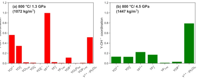
![Figure 3.11: (a-d) Comparison of the aqueous species stability derived from the AIMD simulation and HKF regression using the DEW model [Sverjensky et al., 2014] at 800 C and a fluid density of 1072 kg/m 3 and 1447 kg/m 3 .](https://thumb-eu.123doks.com/thumbv2/1library_info/3689982.1505502/71.918.145.781.142.657/figure-comparison-aqueous-species-stability-simulation-regression-sverjensky.webp)