Takeover Times of Noisy Non-Generational Selection Rules that Undo Extinction

(1)

Takeover Times of Noisy Non-Generational Selection Rules that Undo Extinction

G unter Rudolph

1 Abstract

The takeover time of some selection method is the expected number of iterations of this selec- tion method until the entire population consists of copies of the best individual under the assumption that the initial population consists of a single copy of the best individual. We consider a class of non- generational selection rules that run the risk of loos- ing all copies of the best individual with positive probability. Since the notion of a takeover time is meaningless in this case these selection rules are modied in that they undo the last selection opera- tion if the best individual gets extinct from the pop- ulation. We derive exact results or upper bounds for the takeover time for three commonly used se- lection rules via a random walk or Markov chain model. The takeover time for each of these three selection rules is O(nlogn) with population size n.

1. Introduction

The notion of the takeover time of selection meth- ods used in evolutionary algorithms was introduced by Goldberg and Deb [1]. Suppose that a nite pop- ulation of size n consists of a single best individual and n

^;

1 worse ones. The takeover time of some selection method is the expected number of itera- tions of the selection method until the entire popu- lation consists of copies of the best individual. Evi- dently, this denition of the takeover time becomes meaningless if all best individuals may get extinct with positive probability. Therefore we study a spe- cic modication of those selection rules: If the all best individual have been erased by erroneous se- lection then these selection rules undo this extinc- tion by reversing the last selection operation. Here, we concentrate on non-generational selection rules.

For such rules Smith and Vavak [2] numerically de- termined the takeover time or takeover probability based on a Markovian model whereas Rudolph [3]

oered a theoretical analysis via the same Marko- vian model. This work is an extension of [2, 3] as the modied selection rules introduced here have not been considered yet.

Section 2 introduces the particular random walk

1

Department of Computer Science, University of Dort- mund, Germany; e-mail: guenter.rudolph@udo.edu

model, which reects our assumptions regarding the selection rules, and our standard machinery for de- termining the takeover time or bounds thereof. Sec- tion 3 is of preparatory nature as it contains sev- eral auxiliary results required in section 4 in which our standard machinery is engaged to provide the takeover times for our modications of random re- placement selection, noisy binary tournament se- lection, and \kill tournament" selection. Finally, section 5 relates our ndings to results previously obtained for other selection methods.

2. Model

Let N t denote the number of copies of the best indi- vidual at step t

0. The random sequence (N t ) t

⁰

with values in S =

^f

1;2;:::;n

^g

and N

⁰

= 1 is termed a Markov chain if

Pf

N t

⁺¹

= j

^j

N t = i;N t

^;1

= i t

^;1

;:::;N

⁰

= i

⁰^g

=

Pf

N t

⁺¹

= j

^j

N t = i

^g

= p ij

for all t

0 and for all pairs (i;j)

²

S

S. Since we are only interested in non-generational selection rules the associated Markov chains reduce to par- ticular random walks that are amenable to a the- oretical analysis. These random walks are charac- terized by the fact that

^j

N t

^;

N t

⁺¹^j

1 for all t

0 as a non-generational selection rule chooses|

somehow|an individual from the population and decides|somehow|which individual should be re- placed by the previously chosen one.

Two special classes of random walks were consid- ered in [3] in this context. Here, we need another class reecting our assumption that the selection rules undo a potential extinction of the best individ- ual by reversing the last selection operation. This leads to a random walk with one reecting and one absorbing boundary which is a Markov chain with state space S =

^f

1;:::;n

^g

and transition matrix

P =

0

B

@

r

¹

q

¹

0

0 p

²

r

²

q

²

0

0 0 p

³

r

³

q

³

0

0 ... ... ... ... ... ... ...

0 0 p n

^;2

r n

^;2

q n

^;2

0 0

0 p n

^;1

r n

^;1

q n

^;1

0 0 0 1

1

C

A

1

(2)

with p i ;q i > 0, r i

0, p i + r i + q i = 1 for i = 2;:::;n

^;

1 and r

¹

= 1

^;

q

¹ ²

(0;1). Notice that state n is the only absorbing state. The expected absorption time is

^E

[T

^j

N

⁰

= k ] with T = min

^f

t

0 : N t = n

^g

and it can be determined as follows [4].

Let matrix Q result from matrix P by deleting its last row and column. If C is the inverse of matrix A = I

^;

Q with unit matrix I, then

^E

[T

^j

N

⁰

= k ] = c k

¹

+c k

²

+

+c k;n

^;1

for 1

k < n. Since N

⁰

= 1 in the scenario considered here, we only need the rst row of matrix C = A

^;1

which may be obtained via the adjugate of matrix A. This avenue was followed in Rudolph [5] for a more general situation. Using the result obtained in [5] (by setting p

¹

= 0) we immediately get

c

¹

j =

n

^;X

j

^;1

k

⁼⁰

0

@

n

^;^Y

k

^;1

u

⁼

j

⁺¹

p u

1

A

n

^Y^;1

v

⁼

n

^;

k q u

!

n

^Y^;1

k

⁼

j q k

(1) for 1

j

n

^;

1. Thus, the plan is as follows:

First, derive the transition probabilities for a non- generational selection rule that fullls our assump- tions. This is usually easy. Next, these expressions are fed into equation (1) yielding c

¹

j . The result may be a complicated formula; in this case it will be bounded in an appropriate manner. Finally, we determine the sum

E

[T

^j

N

⁰

= 1] = ⁿ

^X^;1

j

⁼¹

c

¹

j

and we are done. For the sake of notational conve- nience we shall omit the conditioning

^f

N

⁰

= 1

^g

and write simply

^E

[T ] for the expected takeover time.

3. Mathematical Prelude

In case of positive integers the Gammafunction ;(

) obeys the relationships n;(n) = ;(n+1) = n!. For later purposes we need the following results:

Lemma 1 For n

²

IN,

n

^X^;1

k

⁼⁰

;(n + k + 1)

;(k + 1) = ;(2n + 1) (n + 1);(n) :

Proof: See [3], p. 905.

Lemma 2 Let n

2 and 1

j

n

^;

1. Then S(n;j) = n

²

;(n

^;

j);(n + j)

;(j + 1);(2n

^;

j + 1)

n

^;^X

j

^;1

k

⁼⁰

d k

1 2+ 1 4n where

d k = ;(n + k + 1);(n

^;

k)

;(2n

^;

k);(k + 1) :

Proof: Due to lack of space we only oer a sketch of the proof. First show that S(n;0)

S(n;j) for j = 1;:::;n

^;

1 and n

2. Since the bound

2S(n;0) = n ;(n) ;(2n)

²

n

^X^;1

k

⁼⁰

d k

1 + 12n follows from [3], pp. 907-908, division by 2 yields the result desired.

Moreover, the nth harmonic number H n can be bracketed by

logn < H n =

^X

ⁿ

i

⁼¹

1 i < logn + 1 for n

2 and notice that

n

X

i

⁼⁰

a ⁿ

^;

ⁱ b ⁱ = a ⁿ

⁺¹^;

b ⁿ

⁺¹

a

^;

b

for a

⁶

= b. Finally some notation: The set I _nm de- notes all integers between m and n (inclusive).

4. Analysis

4.1. Random Replacement Selection

Two individuals are drawn at random and the bet- ter one of the pair replaces a randomly chosen in- dividual from the population. If the last best indi- vidual was erased by chance then the last selection operation is reversed. As a consequence, the tran- sition probabilities of the associated Markov chain are p nn = 1, p

¹¹

= 1

^;

p

¹²

,

8

i

²

I

¹

ⁿ

^;1

: p i;i

⁺¹

= in

2

^;

i n

1

^;

i n

8

i

²

I

²

ⁿ

^;1

: p i;i

^;1

=

1

^;

i n

2

i n

and p ii = 1

^;

p i;i

^;1^;

p i;i

⁺¹

. Since p i = p i;i

^;1

, q i = p i;i

⁺¹

and

n

^Y^;1

v

⁼

n

^;

k q _v = 1

n

³

^k

⁺¹

;(n + k + 1);(k + 1)

;(n

^;

k) (2)

n

^;^Y

k

^;1

u

⁼

j

⁺¹

p u = 1

n

³⁽

ⁿ

^;

^k

^;

^j

^;1)

;(n

^;

j)

²

;(j + 1) ;(n

^;

k)

;(k + 1)

²

one obtains

n

^;^X

j

^;1

k

⁼⁰

0

@

n

^;^Y

k

^;1

u

⁼

j

⁺¹

p u

1

A

n

^Y^;1

v

⁼

n

^;

k q u

!

= n

³⁽

ⁿ

^;

1 ^j

^;1)+1

;(n

^;

j)

²

;(j + 1)

n

^;^X

j

^;1

k

⁼⁰

;(n + k + 1)

;(k + 1) =

2

(3)

n

³⁽

ⁿ

^;

1 ^j

^;1)+1

;(n

^;

j)

;(j + 1) ;(2n

^;

j + 1)

n + 1 (3)

with the help of Lemma 1. Insertion of k = n

^;

j in equation (2) leads to

n

^Y^;1

v

⁼

j q v = ;(2n

^;

j + 1);(n

^;

j + 1)

n

³⁽

ⁿ

^;

^j

⁾⁺¹

;(j) : (4) After insertion of equations (3) and (4) in equation (1) we have

c

¹

_j = n n + 1

³

1 j

1 n

^;

j = n

²

n + 1

1 j + 1

n

^;

j

and nally

E

[T ] = ⁿ

^X^;1

j

⁼¹

c

¹

j = 2n n + 1 H

²

ⁿ

^;1

:

4.2. Noisy Binary Tournament Selection

Two individuals are drawn at random and the best as well as worst member of this sample is identied.

The worst member replaces the best one with some replacement error probability

²

(0;

¹²

), whereas the worst one is replaced by the best one with prob- ability 1

^;

. Again, if the last best copy has been discarded then the last selection operation is re- versed. Therefore the transition probabilities are as follows: p nn = 1, p

¹²

= s

¹

(1

^;

), p

¹¹

= 1

^;

p

¹²

and p i;i

⁺¹

= s i (1

^;

), p i;i

^;1

= s i , p ii = 1

^;

s i

for i = 2;:::;n

^;

1. Here, s i denotes the probabil- ity that the sample of two individuals contains at least one best as well as one worse individual from a population with i = 1;:::;n

^;

1 copies of the best individual, i.e.,

s i = 1

^;

i n

2

;

1

^;

i n

2

= 2 in

1

^;

i n

: According to equation (1) we need

n

^Y^;1

v

⁼

n

^;

k q v =

2(1

^;

) n

²

k ;(n);(k + 1)

;(n

^;

k)

n

^;^Y

k

^;1

u

⁼

j

⁺¹

p u =

2 n

²

2(

n

^;

j

^;1;

k

⁾

;(n

^;

k);(n

^;

j)

;(k + 1);(j + 1) leading to

n

^;X

j

^;1

k

⁼⁰

0

@

n

^;^Y

k

^;1

u

⁼

j

⁺¹

p u

1

A

n

^Y^;1

v

⁼

n

^;

k q u

!

= 2 ⁿ

^;

^j

^;1

n

²⁽

ⁿ

^;

^j

^;1)

;(n);(n

^;

j)

;(j + 1)

n

^;X

j

^;1

k

⁼⁰

ⁿ

^;

^j

^;1;

^k (1

^;

) ^k = 2 ⁿ

^;

^j

^;1

n

²⁽

ⁿ

^;

^j

^;1)

;(n);(n

^;

j)

;(j + 1)

(1

^;

) ⁿ

^;

^j

^;

ⁿ

^;

^j

1

^;

2 : (5)

Since

n

^Y^;1

v

⁼

j q v =

2(1

^;

) n

²

n

^;

j

;(n);(n

^;

j + 1)

;(j) (6)

we get by inserting equations (5) and (6) into equa- tion (1)

c

¹

j = n 2

²

;(j)

;(j + 1)

;(n

^;

j)

;(n

^;

j + 1)

(1

^;

) ⁿ

^;

^j

^;

ⁿ

^;

^j (1

^;

) ⁿ

^;

^j (1

^;

2)

= n 2

²

1 j

1 n

^;

j

1

^;

2 (1

^;

r ⁿ

^;

^j ) where r = =(1

^;

) and nally

E

[T ] = ⁿ

^X^;1

j

⁼¹

c

¹

j = n

²

2

1

^;

2 n

^;1

X

j

⁼¹

1 j

1 n

^;

j

"

1

^;

1

^;

n

^;

j

^#

= 2(1

^;

n 2)

n

^X^;1

j

⁼¹

1 j + 1

n

^;

j

"

1

^;

1

^;

n

^;

j

^#

= 1

^;

n 2

2

4

H n

^;1^;

1 2

n

^;1

X

j

⁼¹

r ⁿ

^;

^j j

^;

1

2 n

^;1

X

j

⁼¹

r ⁿ

^;

^j n

^;

j

3

5

1

^;

n 2

2

4

H n

^;1^;

1 n

n

^;1

X

j

⁼¹

r ^j

3

5

= 1

^;

n 2

H n

^;1^;

1 n

r

^;

r ⁿ 1

^;

r

nH n

^;1

1

^;

2 where r = =(1

^;

)

²

(0;1). The above bound is very accurate if is not too close to 1=2. For example, for

= 12

^;

1 2n ^k

this bound yields

^E

[T ]

n ^k

⁺¹

H n

^;1

for k

0 whereas the worst case ( = 1=2) reveals

¹

that

E

[T ]

n

²

H n

^;1

for

²

[0;1=2]. Moreover, no- tice that we get

^E

[T ] = nH n

^;1

in the best case ( = 0) [3].

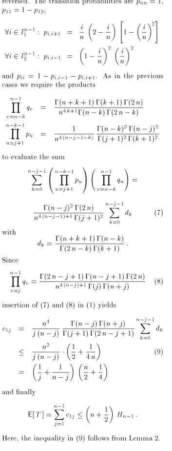
4.3. \Kill Tournament" Selection

This selection method proposed in [2] is based on two binary tournaments: In the rst tournament the best individual is identied. This individual re- places the worst individual identied in the second tournament (the \kill tournament"). If the last best copy gets lost then the last selection operation is

1

If

= 1

⁼

2 then the entire derivation collapses to simple expressions leading to

^E

[

^T

] =

ⁿ²^Hn;1

.

3

(4)

reversed. The transition probabilities are p nn = 1, p

¹¹

= 1

^;

p

¹²

,

8

i

²

I

¹

ⁿ

^;1

: p i;i

⁺¹

= in

2

^;

i n

"

1

^;

i n

2

#

8

i

²

I

²

ⁿ

^;1

: p i;i

^;1

=

1

^;

i n

2

i

n

2

and p ii = 1

^;

p i;i

^;1^;

p i;i

⁺¹

. As in the previous cases we require the products

n

^Y^;1

v

⁼

n

^;

k q v = ;(n + k + 1);(k + 1);(2n) n

⁴

^k

⁺¹

;(n

^;

k);(2n

^;

k)

n

^;^Y

k

^;1

u

⁼

j

⁺¹

p u = 1

n

⁴⁽

ⁿ

^;

^j

^;1;

^k

⁾

;(n

^;

k)

²

;(n

^;

j)

²

;(j + 1)

²

;(k + 1)

²

to evaluate the sum

n

^;^X

j

^;1

k

⁼⁰

0

@

n

^;^Y

k

^;1

u

⁼

j

⁺¹

p u

1

A

n

^Y^;1

v

⁼

n

^;

k q u

!

=

;(n

^;

j)

²

;(2n) n

⁴⁽

ⁿ

^;

^j

^;1)+1

;(j + 1)

²

n

^;X

j

^;1

k

⁼⁰

d k (7) with d k = ;(n + k + 1);(n

^;

k)

;(2n

^;

k);(k + 1) : Since

n

^Y^;1

v

⁼

j q _v = ;(2n

^;

j + 1);(n

^;

j + 1);(2n) n

⁴⁽

ⁿ

^;

^j

⁾⁺¹

;(j);(n + j) (8) insertion of (7) and (8) in (1) yields

c

¹

j = n

⁴

j (n

^;

j) ;(n

^;

j);(n + j)

;(j + 1);(2n

^;

j + 1)

n

^;X

j

^;1

k

⁼⁰

d k

n

²

j (n

^;

j)

1 2 + 1

4n

(9)

=

1 j + 1

n

^;

j

n 2 + 1 4

and nally

E

[T ] = ⁿ

^X^;1

j

⁼¹

c

¹

j

n + 12

H n

^;1

: Here, the inequality in (9) follows from Lemma 2.

5. Summary

Now we are in the position to compare the takeover times of the selection methods considered here with those examined in [3]. Table 1 oers an overview of the takeover times of replace worst selection (RW), quaternary (QT), ternary (TT) and binary (BT)

selection method takeover time

QT

¹²

nH _n

^;1

RW

¹²

nH

²

_n

^;1

TT

²³

nH _n

^;1

BT nH _n

^;1

KT _u

(n +

¹²

)H _n

^;1

BT _u (

¹⁴

)

2nH _n

^;1

RR u

²

n

⁺¹

n

²

H n

^;1

BT u (

¹²

) n

²

H n

^;1

Table 1: Survey of takeover times.

tournament selection with = 0 [3], and kill tour- nament \with undoing" (KT u ), random replace- ment selection \with undoing" (RR u ) and noisy bi- nary tournament selection \with undoing" and re- placement error (BT u ()). For xed < 1=2 the takeover times of all non-generational selec- tion rules considered here and in [3] are of order O(nlogn). Consequently, it does not matter which selection rule is used, provided that the takeover time is actually a key gure of the selection pres- sure.

Acknowledgments

This work was supported by the Deutsche Forschungsgemeinschaft (DFG) as part of the Col- laborative Research Center \Computational Intelli- gence" (

http://sfbci.uni-dortmund.de

).

References

[1] D. E. Goldberg and K. Deb, \A comparative analysis of selection schemes used in genetic algorithms," in Foundations of Genetic Algo- rithms (G. J. E. Rawlins, ed.), pp. 69{93, San Mateo (CA): Morgan Kaufmann, 1991.

[2] J. Smith and F. Vavak, \Replacement strate- gies in steady state genetic algorithms: Static environments," in Foundations of Genetic Al- gorithms 5 (W. Banzhaf and C. Reeves, eds.), pp. 219{233, San Francisco (CA): Morgan Kauf- mann, 1999.

[3] G. Rudolph, \Takeover times and probabilities of non-generational selection rules," in Proceed- ings of the Genetic and Evolutionary Compu- tation Conference (GECCO 2000) (D. Whitley et al. , eds.), pp. 903{910, San Fransisco (CA):

Morgan Kaufmann, 2000.

[4] M. Iosifescu, Finite Markov Processes and Their Applications . Chichester: Wiley, 1980.

[5] G. Rudolph, \The fundamental matrix of the general random walk with absorbing bound- aries," Technical Report CI-75 of the Collabo- rative Research Center \Computational Intelli- gence", University of Dortmund, October 1999.