Observability of Sudden Aerosol Injections by Ensemble-Based Four-Dimensional
Assimilation
of Remote Sensing Data
I n a u g u r a l – D i s s e r t a t i o n zur
Erlangung des Doktorgrades
der Mathematisch–Naturwissenschaftlichen Fakultät der Universität zu Köln
vorgelegt von
Anne Caroline Lange
aus Aachen
Jülich, 2018
Tag der mündlichen Prüfung: 02.03.2018
Die theoretische Vernunft erkennt, „was da ist“, die praktische Vernunft hingegen erschließt, „was da sein soll“.
nach Immanuel Kant [1724–1804]
Abstract
For sudden, often hazardous aerosol injections such as volcanic eruptions, wild fires, and mineral dust uplifts, uncertainties of emission source parameters impose the characterizing impediment for skillful numerical simulations. Large amounts of acci- dentally emitted aerosols can infer serious impacts on health, climate, environment, and economy. This highlights the societal need for reliable forecasts of released particulate matter. Data assimilation and inverse modeling methods incorporate the knowledge gained from both numerical modeling and observations. Applying spatio- temporal assimilation techniques, the combination of the atmospheric dynamics with observations induces constraints with potentially advantageous effects on the simu- lations. Furthermore, ensemble-based analyses provide valuable information about the skill of the forecast results. However, predictions remain uncertain in regions, where observational information is restricted. Confining factors are manifold and include the inaccessibility of observational infrastructure, limitations of measurement configurations or retrieval feasibility, as well as obstructing meteorological conditions, such as clouds, which may strongly restrict remote sensing of aerosols. The research field of observability investigates the impact of utilized observations, thus focusing on observation network optimization and information quantity specification.
Taking the most challenging case of volcanic eruption as prototype example for sudden aerosol injections, the research described in this thesis develops and investigates new methodologies to assess the impact of observations on the analysis. The emphasis is placed on assimilation-based analyses applying both initial value and emission factor optimization for volcanic ash dispersion predictions. As observational input, two entirely different satellite-borne remote sensing principles are exploited: firstly, verti- cally integrated SEVIRI (Spinning Enhanced Visible and Infrared Imager) volcanic ash column mass loadings and secondly, vertically resolved CALIOP (Cloud-Aerosol Lidar with Orthogonal Polarization) particle extinction coefficient profiles. For the assimilation within the EURAD-IM (European Air pollution Dispersion-Inverse Model) system, appropriate observation operators and their adjoint realizations are constructed. The basic theoretical principles of observability in case of volcanic ash column mass loading observations are deduced from the viewpoint of the Kolmogorov- Sinai entropy. The practical analyses are presented for the Eyjafjallajökull eruption event in April 2010. Ensemble versions of both the four dimensional variational (4D- var) data assimilation technique and the particle smoother approach are implemented and processed, able to identify regions of high and low uncertainty in the dispersion simulation results. The analyses reveal a considerable constraining impact of SEVIRI
retrievals to the ash dispersion, while CALIOP retrievals append information only on a very local scale. It is not possible to make a statement on the difference of the resulting quality of the various ensemble simulations due to the following reasons:
firstly, the differences of the assimilation approaches of 4D-var and particle smoother algorithms and secondly, the evaluation of the single Eyjafjallajökull scenario only.
The variable degree of reliability is shown as a consequence of cloud cover dependent observability from space for both quasi-continuous SEVIRI data and sparse CALIOP overpasses.
Kurzzusammenfassung
Im Falle unerwarteter und häufig auch gefährlicher Aerosolemissionen wie beispiels- weise Vulkanausbrüche, Waldbrände und Mineralstaubaufwirbelungen führen deren unsichere Quellparameterabschätzungen zu charakteristischen Schwierigkeiten bei der Erstellung geeigneter numerischer Simulationen. Große Mengen plötzlich emit- tierter Aerosole können ernsthafte Folgen für Gesundheit, Klima, Umwelt und Wirtschaft nach sich ziehen. Daraus ergibt sich die gesellschaftliche Notwendigkeit, verlässliche Ausbreitungsvorhersagen von freigesetzten Partikelansammlungen in der Atmosphäre bereitzustellen. Methoden der Datenassimilation und inversen Model- lierung verbinden die Erkenntnisse, die sowohl aus numerischer Modellierung als auch aus Beobachtungen gewonnen werden. Die Anwendung raum-zeitlicher Assimilations- techniken nutzt die Verbindung von atmosphärischer Dynamik mit unterschiedlichsten Beobachtungen. Daraus können sich Korrekturen ergeben, die potentiell vorteilhafte Effekte auf die Simulationen verursachen. Darüber hinaus erbringen ensemblebasierte Analysen wertvolle Informationen über die Güte der Vorhersageergebnisse. Diese Prognosen bleiben jedoch unsicher für Regionen, in denen Beobachtungsinforma- tionen eingeschränkt verfügbar sind. Begrenzende Faktoren gibt es viele. Zum Beispiel: Unzugänglichkeiten für Beobachtungsinfrastrukturen, Einschränkungen bei Messkonfigurationen oder eingeschränkte Retrievalumsetzbarkeiten sowie störende meteorologische Bedingungen. Zu letzteren zählen insbesondere Wolken, die Fern- erkundungsbeobachtungen von Aerosolen stark behindern. Das Forschungsgebiet der Beobachtbarkeit untersucht den Einfluss von Beobachtungen und konzentriert sich dabei auf die Optimierung von Beobachtungsnetzwerken und auf die Ermittlung des zugehörigen Informationsumfangs.
In Anwendung einer vulkanischen Eruption als besonders anspruchsvoller Proto- typ für plötzliche Aerosolereignisse entwickelt und untersucht die in dieser Arbeit beschriebene Forschung neue Methodiken, den Einfluss von Beobachtungen auf die Analyse zu bewerten. Dabei liegt der Schwerpunkt auf assimilationsbasierten Analysen unter Verwendung von Anfangswert- und Emissionsfaktoroptimierung für Vulkanasche-Ausbreitungsvorhersagen. Als Beobachtungs-Dateneingabe werden zwei völlig verschiedene Satelliten gestützte Fernerkundungsprinzipien genutzt: einerseits vertikal integrierte SEVIRI (Spinning Enhanced Visible and Infrared Imager) Vul- kanaschemassen in einer definierten Säule, andererseits vertikal aufgelöste CALIOP (Cloud-Aerosol Lidar with Orthogonal Polarization) Partikelextinktionskoeffizienten-
Profile. Für die Assimilation im EURAD-IM-System (European Air pollution Dispersion-Inverse Model) werden entsprechende Beobachtungsoperatoren und deren
adjungierte Versionen entwickelt. Die theoretischen Grundsätze der Beobachtbarkeit im Falle von Beobachtungen von Vulkanasche-Massesäulen sind aus der Perspektive der Kolmogorov-Sinai-Entropie abgeleitet. Die praktischen Analysen werden für das Eyjafjallajökull-Ausbruchsereignis im April 2010 aufgezeigt. Ensembleversionen einerseits mit vier-dimensionaler variationeller (4D-var) Datenassimilationstechnik und andererseits mit „particle smoother“-Ansatz werden implementiert und ausge- führt. Durch die Simulationsergebnisse lassen sich Regionen identifizieren, die hohe bzw. niedrige Unsicherheiten der Partikelausbreitung aufzeigen. Die vorgenommenen Analysen weisen eine deutlich beschränkende Wirkung der SEVIRI-Retrieval auf die Ascheausbreitung auf, während die CALIOP-Retrieval gewisse Informationen auf sehr lokalen Skalen beitragen. Wegen der unterschiedlichen Assimilationsan- sätze von 4D-var gegenüber „particle smoother“-Algorithmen kann auf Basis des einzigen Eyjafjallajökull-Szenarios keine Aussage über die Unterschiede der Ergeb- nisqualität von den Ensemblesimulationen getroffen werden. Der variable Grad der Verlässlichkeit resultiert aus der bewölkungsabhängingen Beobachtbarkeit aus dem Weltall sowohl seitens der quasi-kontinuierlichen SEVIRI-Daten als auch der vereinzelten CALIOP-Überflüge.
Contents
Abstract v
Kurzzusammenfassung vii
List of Figures xi
List of Tables xv
Acronyms xvii
1 Introduction 1
2 Observability of sudden aerosol injections 7
2.1 Observability . . . 7
2.1.1 Observability in atmospheric applications . . . 8
2.1.2 Analyzing observability . . . 10
2.2 Monitoring aerosols . . . 15
2.3 Special aerosol events . . . 18
3 Data Assimilation 21 3.1 Four dimensional variational data assimilation . . . 21
3.2 Ensemble data assimilation via particle smoother . . . 24
4 Observations 27 4.1 SEVIRI . . . 27
4.1.1 Instrumentation and measurement configuration . . . 27
4.1.2 Volcanic ash mass loading retrieval . . . 29
4.1.3 Advantages and disadvantages . . . 31
4.2 CALIOP . . . 32
4.2.1 Instrumentation and measurement configuration . . . 32
4.2.2 Aerosol extinction coefficient retrieval . . . 34
4.2.3 Advantages and disadvantages . . . 36
5 Modelling system 39 5.1 EURAD-IM . . . 39
5.2 ESIAS-Chem . . . 43
6 Developments 45
6.1 Model domain . . . 45
6.2 The SEVIRI observation operator . . . 46
6.3 The CALIOP observation operator . . . 47
6.4 Observability analysis with ESIAS . . . 49
7 Observability Analyses 51 7.1 General experiment setup . . . 52
7.1.1 Aerosol scenario . . . 52
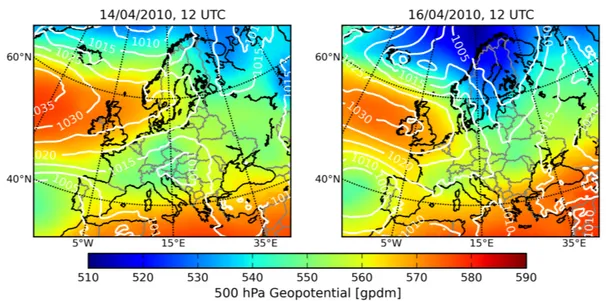
7.1.2 Meteorological conditions . . . 53
7.1.3 Ensemble generation . . . 55
7.1.4 Error assessment . . . 57
7.2 4D-var ensemble using SEVIRI retrievals . . . 58
7.3 4D-var ensemble using SEVIRI and CALIOP retrievals . . . 68
7.4 ESIAS-chem ensemble using SEVIRI retrievals . . . 75
8 Conclusion and Outlook 83 General Acknowledgments 87 A Appendix 89 A.1 Supplements to the 4D-var ensemble analysis using SEVIRI retrievals 89 A.2 Supplements to the 4D-var ensemble analysis using SEVIRI and CALIOP retrievals . . . 93
A.3 Supplements to the ESIAS-chem ensemble analysis using SEVIRI retrievals . . . 98
Bibliography 99
Personal Acknowledgments 117
List of Figures
2.1 Illustration of the Kolmogorov-Sinai entropy . . . 11
4.1 Artist’s view of Meteosat Second Generation in space . . . 28
4.2 MSG-SEVIRI’s total field of view and area of retrieved volcanic ash data set . . . 31
4.3 Artist’s view of CALIPSO in space . . . 33
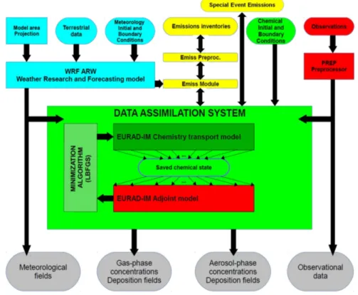
5.1 Flow chart of the EURAD-IM model system . . . 40
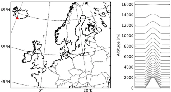
6.1 Model domain and vertical grid resolution . . . 46
7.1 Explosive eruption of the Eyjafjallajökull on 16 April 2010 . . . 52
7.2 Meteorological situation in Europe during the Eyjafjallajökull eruption 53 7.3 Cloud cover above Europe during the Eyjafjallajökull eruption illus- trated by MODIS natural color images from 14–17 April 2010 . . . . 54
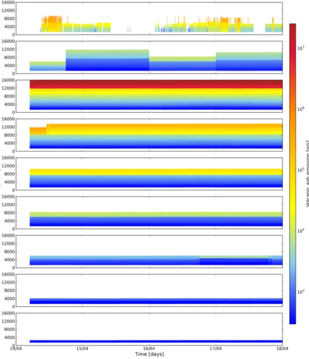
7.4 Volcanic ash emission profiles of the 4D-var ensemble . . . 56
7.5 MSG-SEVIRI volcanic ash column mass loading retrievals of the Eyjafjallajökull 2010 ash plume on 15–17 April . . . 58
7.6 Comparison of PM10 time series of the 4D-var ensemble first guesses and analyses (based on SEVIRI data) with independent observations at Schneefernerhaus on 17 April 2010 . . . 59
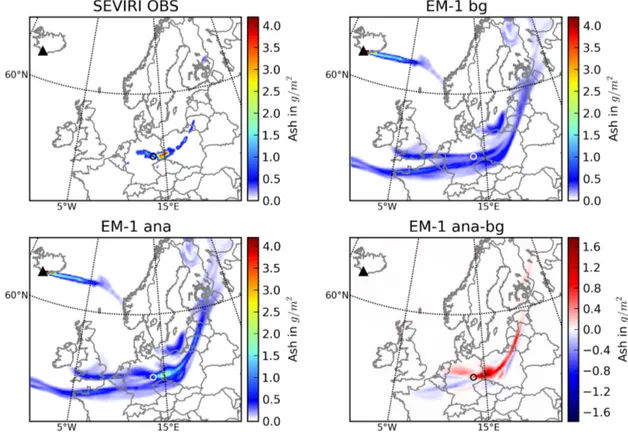
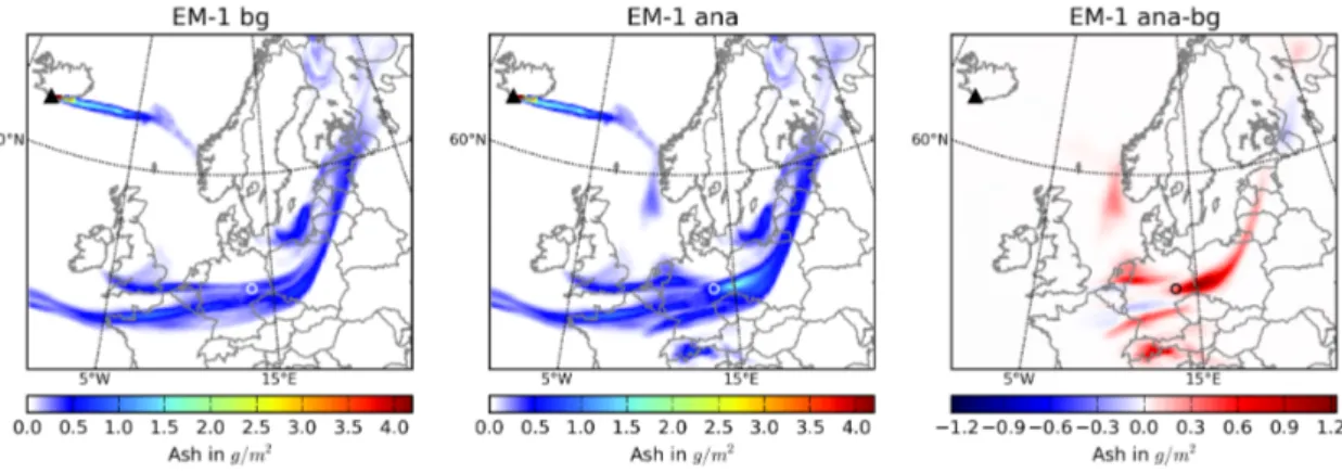
7.7 Horizontal volcanic ash distribution above Europe on 16 April at 13 UTC, as retrieved from SEVIRI observations, EM-1 background field, EM-1 analysis field applying 4D-var assimilation of SEVIRI data, and the analysis increment . . . 60
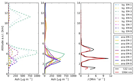
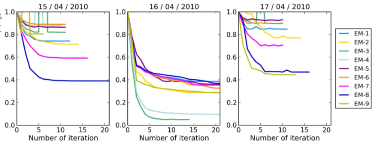
7.8 Vertical volcanic ash distribution over Leipzig on 16 April at 13 UTC: Concentration profiles of the background and analysis fields (based on SEVIRI data) of the 4D-var ensemble, as well as the lidar retrieved mean backscatter coefficient profiles of the Leipzig EARLINET station 62 7.9 Volcanic ash column mass loadings at the EARLINET station in Leipzig on 16 April at 13 UTC: background and analysis (based on SEVIRI data) of the 4D-var ensemble, the analysis ensemble mean, SEVIRI pixels and their mean, and lidar derived mass loading equivalent 63 7.10 Iterative evolution of normalized cost function for the nine members of the 4D-var ensemble, based on the assimilation of SEVIRI data . . 64
7.11 Spaghetti plots of 1.0 g m−2mass isopleths for all nine 4D-var ensemble members: first guess and analysis (based on SEVIRI data) are depicted on 15 April at 12 UTC, 16 April at 12 UTC, and 17 April at 04 UTC . 65 7.12 Spaghetti plots of 0.2 mg m−3 and 2.0 mg m−3 volcanic ash concentra-
tion isopleths as vertical cross section for all nine 4D-var ensemble members: first guess and analysis (based on SEVIRI data) on 16 April at 12 UTC . . . 67 7.13 CALIPSO ground tracks of all available overpasses in the model
domain on 15–17 April . . . 69 7.14 Comparison of PM10 time series of the 4D-var ensemble first guesses
and analyses (based on SEVIRI and CALIOP data) with independent observations at Schneefernerhaus on 17 April 2010 . . . 69 7.15 Horizontal volcanic ash distribution above Europe on 16 April at
13 UTC: EM-1 background field, EM-1 analysis field applying 4D-var assimilation of SEVIRI and CALIOP data, and the analysis increment 70 7.16 Vertical volcanic ash distribution over Leipzig on 16 April at 13 UTC:
Concentration profiles of the analysis shown in Figure 7.8 and of the analysis applying combined SEVIRI and CALIOP retrievals, as well as the mass equivalent derived from the lidar profile of the Leipzig EARLINET station . . . 71 7.17 Volcanic ash column mass loadings at the EARLINET station in
Leipzig on 16 April at 13 UTC: analysis ensemble mean (based on SE- VIRI data), analysis ensemble mean (based on SEVIRI and CALIOP data), SEVIRI observation mean, and lidar derived mass loading equivalent . . . 71 7.18 Spaghetti plots of 1.0 g m−2mass isopleths for all nine 4D-var ensemble
members: first guess and analysis (based on SEVIRI and CALIOP data) are depicted on 15 April at 12 UTC, 16 April at 12 UTC, and 17 April at 04 UTC . . . 73 7.19 Comparison of assimilated CALIOP particle extinction retrievals with
spaghetti plots of 0.2 mg m−3 volcanic ash concentration isopleths as vertical cross section along the 16 April 01:20 UTC CALIPSO overpass.
The mass isopleths are depicted for the first guess, the analysis (based on SEVIRI data), and the analysis (based on SEVIRI and CALIOP data) on 16 April at 01 UTC . . . 74 7.20 Spaghetti plots of 1.0 g m−2 volcanic ash column mass loadings for
the PS ensemble analysis with 60 ensemble members on 15 April at 12 UTC, 16 April at 12 UTC, and 17 April at 04 UTC . . . 76 7.21 MSG-SEVIRI volcanic ash column mass loading retrievals on 16 April
at 00 UTC . . . 77 7.22 Spaghetti plots of 1.0 g m−2 volcanic ash column mass loadings of
with 60 ensemble members on 16 April at 00 UTC: the PS ensemble analysis based on the assimilation of all available SEVIRI data and SEVIRI retrievals higher than 0.45 g m−2 . . . 78
LIST OF FIGURES xiii
7.23 Ensemble mean and ensemble spread for the PS ensemble analyses SEVIRI-1 and SEVIRI-2 on 16 April at 00 UTC . . . 78 7.24 Comparison of PM10 observations with the PS ensemble analysis
SEVIRI-2 of volcanic ash concentrations at Schneefernerhaus on 17 April 2010 . . . 79 7.25 Analyzed volcanic ash emission profiles of PS ensemble member 30
between 14 April at 06 UTC to 15 April at 12 UTC . . . 80 A.1 Horizontal ash distribution above Europe on 16 April at 13 UTC as
displayed in Figure 7.7 but for EM-2 (analysis based on SEVIRI data) 89 A.2 Horizontal ash distribution above Europe on 16 April at 13 UTC as
displayed in Figure 7.7 but for EM-3 (analysis based on SEVIRI data) 90 A.3 Horizontal ash distribution above Europe on 16 April at 13 UTC as
displayed in Figure 7.7 but for EM-4 (analysis based on SEVIRI data) 90 A.4 Horizontal ash distribution above Europe on 16 April at 13 UTC as
displayed in Figure 7.7 but for EM-5 (analysis based on SEVIRI data) 91 A.5 Horizontal ash distribution above Europe on 16 April at 13 UTC as
displayed in Figure 7.7 but for EM-6 (analysis based on SEVIRI data) 91 A.6 Horizontal ash distribution above Europe on 16 April at 13 UTC as
displayed in Figure 7.7 but for EM-7 (analysis based on SEVIRI data) 92 A.7 Horizontal ash distribution above Europe on 16 April at 13 UTC as
displayed in Figure 7.7 but for EM-8 (analysis based on SEVIRI data) 92 A.8 Horizontal ash distribution above Europe on 16 April at 13 UTC as
displayed in Figure 7.7 but for EM-9 (analysis based on SEVIRI data) 93 A.9 Horizontal ash distribution above Europe on 16 April at 13 UTC as
displayed in Figure 7.15 but for EM-2 (analysis based on SEVIRI and CALIOP data) . . . 93 A.10 Horizontal ash distribution above Europe on 16 April at 13 UTC as
displayed in Figure 7.15 but for EM-3 (analysis based on SEVIRI and CALIOP data) . . . 94 A.11 Horizontal ash distribution above Europe on 16 April at 13 UTC as
displayed in Figure 7.15 but for EM-4 (analysis based on SEVIRI and CALIOP data) . . . 94 A.12 Horizontal ash distribution above Europe on 16 April at 13 UTC as
displayed in Figure 7.15 but for EM-5 (analysis based on SEVIRI and CALIOP data) . . . 94 A.13 Horizontal ash distribution above Europe on 16 April at 13 UTC as
displayed in Figure 7.15 but for EM-6 (analysis based on SEVIRI and CALIOP data) . . . 95 A.14 Horizontal ash distribution above Europe on 16 April at 13 UTC as
displayed in Figure 7.15 but for EM-7 (analysis based on SEVIRI and CALIOP data) . . . 95 A.15 Horizontal ash distribution above Europe on 16 April at 13 UTC as
displayed in Figure 7.15 but for EM-8 (analysis based on SEVIRI and CALIOP data) . . . 95
A.16 Horizontal ash distribution above Europe on 16 April at 13 UTC as displayed in Figure 7.15 but for EM-9 (analysis based on SEVIRI and CALIOP data) . . . 96 A.17 Iterative evolution of normalized cost function for the nine members
of the 4D-var ensemble, based on the assimilation of SEVIRI and CALIOP data . . . 96 A.18 Spaghetti plots of 0.2 mg m−3 and 2.0 mg m−3 volcanic ash concentra-
tion isopleths as vertical cross section for all nine 4D-var ensemble members: first guess and analysis (based on SEVIRI and CALIOP data) on 16 April at 12 UTC . . . 97 A.19 Spaghetti plots of 1.0 g m−2 volcanic ash column mass loadings for
the PS ensemble analysis SEVIRI-2 with 60 ensemble members on 15 April at 12 UTC, 16 April at 12 UTC, and 17 April at 04 UTC . . . . 98 A.20 Comparison of PM10 observations with the PS ensemble analysis
SEVIRI-1 of volcanic ash concentrations at Schneefernerhaus on 17 April 2010 . . . 98
List of Tables
4.1 Characteristics of SEVIRI’s spectral channels . . . 28 5.1 Trimodal log-normal representation in MADE . . . 42
Acronyms
AOD Aerosol Optical Depth
ARW Advanced Research WRF
A-train Afternoon Train
BLUE Best Linear Unbiased Estimation
CALIOP Cloud-Aerosol Lidar with Orthogonal Polarization
CALIPSO Cloud-Aerosol Lidar and Infrared Pathfinder Satellite Observa- tion
CATS Cloud-Aerosol Transport System
CCN Cloud Condensation Nuclei
CNES Centre National d’Études Spatiales
CTM Chemistry Transport Model
EARLINET European Aerosol Research Lidar Network EarthCARE Earth Clouds, Aerosols and Radiation Explorer
ECMWF European Centre for Medium-Range Weather Forecasts
EEM EURAD Emission Model
EM Ensemble Member
EMEP European Monitoring and Evaluation Programme
ESA European Space Agency
ESIAS Ensemble for Stochastic Integration of Atmospheric Simulations ESIAS-chem Ensemble for Stochastic Integration of Atmospheric Simulations
– Atmospheric Chemistry
ESIAS-met Ensemble for Stochastic Integration of Atmospheric Simulations – Meteorology
EUMETSAT European Organisation for the Exploitation of Meteorological Satellites
EURAD-IM European Air pollution Dispersion–Inverse Model EUROCONTROL European Organisation for the Safety of Air Navigation FASTEX Fronts and Atlantic Storm Track Experiment
FLEXPART Flexible Particle dispersion model
4D-var Four Dimensional Variational data assimilation FSO Forecast Sensitivity of Observations
GOME-2 Global Ozone Monitoring Experiment-2 GMAO Global Modeling and Assimilation Office HERA Hybrid Extinction Retrieval Algorithm
IAGOS In-Service Aircraft for a Global Observing System IASI Infrared Atmospheric Sounding Interferometer IFS Integrated Forecasting System
IIR Imaging Infrared Radiometer
IN Ice Nuclei
IPCC Intergovernmental Panel on Climate Change
KSE Kolmogorov-Sinai Entropy
L-BFGS Limited-memory Broyden-Fletcher-Goldfarb-Shenno algorithm LETKF Localized Ensemble Transform Kalman Filter
Lidar Light Detection and Ranging
LOTOS-EUROS Long Term Ozone Simulation – European Ozone Simulation MADE Modal Aerosol Dynamics model for Europe
MISR Multi-angle Imaging Spectroradiometer
MODIS Moderate Resolution Imaging Spectroradiometer
MSG Meteosat Second Generation
NAME Numerical Atmospheric dispersion Modeling Environment NASA National Aeronautics and Space Administration
NetCDF Network Common Data Form
NWP Numerical Weather Predication
OMI Ozone Monitoring Instrument
OSEs Observing System Experiments
OSSE Observing System Simulation Experiment
PAN Peroxyacetyl Nitrate
PDF Probability Density Function
PS Particle Smoother
Radar Radio Detection and Ranging SCA Scene Classification Algorithm
SEVIRI Spinning Enhanced Visible and Infrared Imager SIBYL Selective, Iterated Boundary Location
SORGAM Secondary Organic Aerosol Model
SVA Singular Vector Analysis
VOCs Volatile Organic Compounds
WFC Wide Field Camera
WMO World Meteorological Organization WRF Weather Research and Forecasting Model
WRF-Chem Weather Research and Forecasting model coupled to Chemistry
1 | Introduction
The Earth’s atmosphere transports and transforms many different aerosols originating from natural and anthropogenic emission sources, which are often dependent on hardly predictable processes. Special aerosol events include for instance wildfires, mineral dust storms, or accidental aerosol releases resulting from damage of industrial plants or reactors. Their sudden appearance in combination with their potential hazards is the reason that skillful predictions of the succeeding aerosol dispersion are indispensable. However, the assessment of meaningful predictions has a major associated challenge: emission parameters and observability, which analyzes the impact of observations on the value of the forecast in a probabilistic manner, must first be adequately quantified. This work particularly focuses on sudden aerosol events, which are characterized by the release of enormous amounts of special aerosol emissions that can cause hazardous outcomes for humans’ health (Pöschl [2005]), and that can negatively affect society (e. g. Chester [2005]) and the environment (e.
g. Thordarson and Self [2003]).
To simulate the aerosol dispersion, numerical models are used. They primarily rest on theoretical knowledge of the atmosphere system. This knowledge generally encompasses the meteorological fields as a basis for the main dynamic terms of advection, dispersion, and deposition. In case of sudden aerosol injections, dispersion models often rely on poorly known emission source describing input parameters, including emission location, emission start and end time, emission mass rate and composition, plume height, and particle size distribution. Consequently, the sum of all these uncertainties involved in the input estimations can lead to large forecast inaccuracies, such that hazard assessments might fail with fatal consequences.
The eruption of the Icelandic volcano Eyjafjallajökull in April and May 2010 can be considered as a prototype exceptional aerosol event. This incident caused a wide-reaching closure of the European air space. The temporary air traffic shutdown resulted in global economical losses of 4.7 billion US-Dollars (Oxford Economics [2010]). The decision to keep airplanes grounded during the volcanic ash dispersion above Europe was mainly based on simulation results of ash dispersion models. Thus in 2010, it was debated if dispersion models even approximate the true atmospheric state, and how reliable these dispersion forecasts are. Explosive volcanic eruptions are aerosol events that are particularly challenging to predict, since their emissions behave in an erratic manner. This is especially momentous because the emission plume height can change drastically within short periods over hundreds to thousands of meters altitude, and the mass eruption rate can vary from kilograms to several
tons of particulate matter per second. This thesis emphasizes the examination of volcanic aerosol events being selected as a paradigm, since it compromises these special challenges. For most considerations related to volcanic eruptions scenarios, analogical characteristics and methods can be identified for other sudden aerosol events.
To estimate the source term of volcanic ash emissions, two approaches are common.
With heuristic emission modules, which rest on statistical analyses of historical eruptions, the total mass emission of the fine ash fraction can be roughly derived from emission plume height information (Mastin et al. [2009]; Suzuki et al. [1983]).
The other procedure includes additional information on the eruption plume’s charac- teristics caused by the prevailing meteorological conditions (Woodhouse et al. [2013];
Folch et al. [2016]).
Observations obtained from a wide range of different sensors can contribute valuable information about the aerosol scenario. Ground-based observations performed near the emission source can directly explore many important source parameters. Cameras observing within the infrared spectral range enable the derivation of microphysical quantities of the ash particles within the eruption plume (Prata and Bernardo[2009]).
Ultraviolet cameras detect sulfur dioxide contained in the plume, such that the precursor amount of sulfate aerosol can be retrieved (Burton et al. [2015]). However, recent studies like Burton [2016] also apply ultraviolet imaging for volcanic ash monitoring. Stohl et al. [2011] used webcam observations to estimate the eruption column top heights of the 2010 Eyjafjallajökull eruption. Weather radar (radio detection and ranging) instruments are capable of capturing volcanic ash plume heights within their detection area during the normal operation of the system, as realized by Arason et al. [2011].
Since volcanic eruptions often occur in remote regions on Earth, where such ob- servational infrastructure is not readily available, observations of volcanic clouds in places remote to the emission source can provide important information about the scenario. Accordingly, Flentje et al. [2010] performed among other observations in situ measurements of particle number concentrations of the volcanic ash that initially arrived in Southern Germany two and a half days after the eruption start of the Eyjafjallajökull. Aircraft based measurements performed on specially equipped research airplanes obtain an unique insight into the transported ash cloud (e. g.
Schumann et al. [2011]). Remote sensing instruments are able to capture a broader picture of the volcanic ash cloud, retrieving ash characteristics from their spectral signature. With lidar (light detection and ranging) measurements, spectral and vertically resolved optical properties of the transported ash were obtained in central Europe during the Icelandic eruption in 2010, and attempts to retrieve the mass concentration within the ash clouds were carried out for instance by Ansmann et al.
[2011] and Gasteiger et al. [2011]. The organization of ground-based instruments in networks is advantageous to attain the four dimensional distributions of volcanic clouds, as realized by Pappalardo et al. [2013] in the framework of EARLINET (European Aerosol Research Lidar Network).
Satellite sensors generally observe the horizontal distribution and extension of vol-
3
canic ash clouds. Here, also infrared instrumentations are primarily favorable to derive ash optical properties and estimates of mass loadings. This has been carried out by e. g. Prata and Prata [2012] using SEVIRI (Spinning Enhanced Visible and Infrared Imager) data and Dubuisson et al. [2014], who applied their retrieval algo- rithm to analyze near simultaneously infrared measurements from SEVIRI, MODIS (Moderate Resolution Imaging Spectroradiometer), and IASI (Infrared Atmospheric Sounding Interferometer). Volcanic ash AOD (aerosol optical depth) and microphys- ical properties observed by MISR (Multi-angle Imaging Spectroradiometer) even indicate aging processes of the ash plume during its transport (Kahn and Limbacher [2012]). Space borne lidar instruments, such as CALIOP (Cloud-Aerosol Lidar with Orthogonal Polarization) or CATS (Cloud-Aerosol Transport System) allow for the determination of the ash cloud height and thickness in addition to optical properties (Winker et al. [2012]), but the assessment is restricted to the re-visitation times and narrow swath of the lidar beam. A full overview of volcanic emission monitoring from space is provided byThomas and Watson [2010].
In principle, observations are subject to limitations that must be considered. In particular, remote sensing retrievals are restricted to cloud clear areas. Furthermore, the discrimination of different aerosol species, and the retrieval of one certain aerosol type are challenging. Vertically integrated measurement quantities are restricted in the way that the three dimensional dispersion within the atmosphere cannot be identified. Consequently, all these limitations add up to initial measurement uncertainties.
The combination of volcanic ash transport and dispersion models with observations can be accomplished by the comparison of model results with measurements or retrievals. For instance,Webley et al. [2012] validated their WRF-Chem (Weather Research and Forecasting model coupled to Chemistry) ash dispersion simulation by means of different observational data from satellite and ground-based platforms.
Another approach to connect models with observations is by inverse modeling and data assimilation. Thus, models can be well constrained in terms of adjusting model states, or in an enhanced way with respect to initial value or emission factor optimization (Elbern et al. [2007], Chap. 2 of Zehner [2010]). This leads to more reliable and more accurate dispersion forecasts, such that the scenario, the associated mechanisms, and subsequent hazards can be assessed. A review of how observations of airborne ash from space are exploited by volcanic ash dispersion modelers is given byWilkins et al. [2016a].
Wilkins et al. [2016c] presented their results of the volcanic ash transport connected with the 2011 Grímsvötn eruption in Iceland using the novel technique of data inser- tion. Further related studies with a focus on the Eyjafjallajökull eruption are given by Wilkins et al. [2014; 2016b]. They initialized NAME (Numerical Atmospheric dispersion Modeling Environment) with SEVIRI ash cloud heights and column ash mass loadings retrieved with the algorithm ofFrancis et al.[2012]. Later on, they up- dated the model state using this retrieved data in addition to probabilistic estimates of ash, cloud, and clear sky classifications described byMackie and Watson [2014].
Assuming an ash layer thickness of 1.0 km and applying satellite retrieved ash cloud heights was demonstrated as most beneficial with respect to the ash transport, while
ash concentrations were predominantly under-predicted. Further, the dynamical system evolution of the model was not appropriately considered. The method can not be applied before retrieved remote sensing data for the initialization is provided.
In that work, the estimation of actual emissions was neglected, as well as observation and model errors.
Eckhardt et al. [2008] and Kristiansen et al. [2010] developed an analytical inversion method in FLEXPART (FLEXible PARTicle dispersion model) to estimate vertical profiles of sulfur dioxide emissions and tested it on the basis of the 2007 Jebel at Tair and the 2008 Kasatochi eruption, respectively. Using satellite-borne total column retrievals, the vertical wind shear of horizontal winds was exploited to extract the emission heights. Stohl et al. [2011] improved this method by extracting vertically and temporally resolved a posteriori emissions, as a linear combination of the best fitting a priori emission scenarios. Model errors derived from the difference of two different meteorological input data sets, and observation errors were taken into account to determine the ash emissions of the Eyjafjallajökull eruption. Kristiansen et al. [2012] and Steensen et al.[2017] applied further configurations, alternatively testing the algorithm with NAME and EMEP (European Monitoring and Evaluation Programme) dispersion models, respectively. Furthermore, Steensen et al. [2017]
explored how different satellite data and uncertainty assumptions affect the volcanic ash emission estimates. To quantify the uncertainties of volcanic ash emissions, Kristiansen et al. [2012] advise an ensemble approach.
Since in the year 2010 the ECMWF’s (European Centre for Medium-Range Weather Forecasts) IFS (Integrated Forecast System) did not contain a volcanic ash aerosol variable,Benedetti et al. [2011] initialized the volcanic emissions applying the emis- sions from Stohl et al.[2011] to the sulfate, black carbon and dust variables. The four dimensional variational (4D-var) analysis of MODIS AOD constrained the volcanic ash plume, especially in regions remote to the source. Regarding volcanic sulfur diox- ide emissions, Flemming and Inness[2013] suggest to combine emission parameter initialization with 4D-var assimilation, both on the basis of satellite retrievals. The initialization was based on an ensemble of test tracers injected in different heights to estimate the plume height for the assimilation. Among other methods, the 4D-var approach provides the best linear unbiased estimate (BLUE, Talagrand[1997]) as optimality criterion, such that the results consider the uncertainties of the model as well as the observations.
Lu et al. [2016] set up an ensemble, where each member was assigned to a specific emission profile. With an adjoint-free trajectory based 4D-var method, the best emission estimation resulted from the weighted ensemble mean. The weights were determined by cost function minimization considering synthetic observations of ash column mass loadings in identical twin experiments. Yet, analysis uncertainty assess- ments were not provided in the article.
Fu et al. [2016] and Fu et al. [2017] assimilated aircraft based measurements and SEVIRI ash column mass loadings, respectively, obtained during the Eyjafjallajökull eruption. They applied an Ensemble-Kalman Filter to the stochastic version of the LOTOS-EUROS (Long Term Ozone Simulation – European Ozone Simulation)
5
model. Thereby, they improved the estimation of the volcanic ash state and argued that the aviation advice could be improved. Nonetheless, this is only justifiable for forecast regions downwind of the assimilated observations and later forecast times.
To assess the hazards associated with volcanic ash clouds, probabilistic methods estimating the forecast uncertainties are applied. For instance,Denlinger et al.[2012]
performed a Bayesian analysis to determine initial conditions and uncertainties with satellite and ground-based observations. In this way, the posterior probability could be derived and proofed as robust, while Gaussian distributed uncertainties were considered.
All these studies demonstrate that inverse modeling and data assimilation overcome the limits of simple forward modeling. Therefore, model calculations are benefi- cially constrained by the observational data. However, the question where and to what extend observations reduce uncertainties is not directly answered, but of high practical interest. Flight route planning in aviation is a striking, yet by far not the only example. Evaluation of improvements regarding analysis quality as a product of observation configurations and data assimilation is the main subject in the research topic of observability (Majumdar[2016]). Interests in this research field include the optimization of observation networks, the evaluation of the quality gain in the analysis due to individual or types of observations, and the appraisal to what extend the analysis can be influenced by observations. A detailed literature review of meteorological and atmospheric chemistry related studies is provided in Chapter 2.1.1.
Regarding special aerosol events, targeted observations can be expected to contribute valuable information about the scenario. Additional information can be gained from the dynamics of the system, such as when taking advantage of the vertical wind shear to estimate the horizontal distribution. However, it has rarely been evaluated which simulated temporal and spatial concentration patterns are actually controlled by observations. This might be an important aspect in consideration of a strong basis for decision making.
This work aims to develop and validate observability methodologies, which identify those areas in the analysis that are well constrained by the information content provided by observations. A related objective is to assess the limits of observability in the analyses obtained. These objectives are pursued with the application of two competing approaches:
• The analysis uncertainty is assessed with an ensemble setup of EURAD-IM (European Air pollution Dispersion – Inverse Model,Elbern et al. [2007]) using the 4D-var data assimilation technique in terms of initial value optimization.
• An ensemble of major size defined with ESIAS-chem (Ensemble for Stochastic Integration of Atmospheric Simulations – atmospheric chemistry part,Franke [2018]) is processed to perform emission factor optimization by means of non-linear particle smoother data assimilation.
These approaches are combined with the employment of two fundamentally different satellite-borne observation principles. On the one hand, SEVIRI retrievals of total ash column mass loadings are used, which are confined to capture the horizontal ash
distribution only. On the other hand, CALIOP retrieved profiles of aerosol extinction coefficients contribute with sparse, but precise vertically resolved data.
This thesis is organized as follows: in the subsequent Chapter 2, a detailed insight into the research field of observability is given. Thereby, particular attention is given to the theory of obtaining the observability of exclusively horizontally resolved observation data. Further, aerosol monitoring and the challenges of sudden aerosol injection dispersion modeling are discussed in Section 2.2 and Section 2.3, respectively.
Chapter 3 introduces the concept of data assimilation, particularly focusing on the applied methods of the 4D-var approach and ensemble-based particle smoother. The aim of Chapter 4 is to introduce the observation systems of CALIOP and SEVIRI including the retrieval description and a discussion of their skills. Chapter 5 describes the modeling system of EURAD-IM as well as the ensemble environment of ESIAS.
In the sequel, Chapter 6 presents the main developments achieved, to properly assimilate the selected remote sensing data and to evaluate the ensemble analysis in terms of observability. In Chapter 7, at first the selected aerosol scenario of the 2010 Eyjafjallajökull eruption and the experiments’ setups are explained, before all performed experiments are analyzed and their results are summarized. The observability of SEVIRI data is investigated with both data assimilation techniques, while the additive information gain due to CALIOP data is at first examined with the 4D-var ensemble. Finally, conclusions are drawn in Chapter 8 and a perspective with suggestions for further investigations and improvements is given.
2 | Observability of
sudden aerosol injections
Within this chapter, the theoretical approach to the term of observability is intro- duced. Applications in atmospheric research are reviewed and analysis theories and techniques related to the question of this thesis are discussed. The subsequent exposition gives a closer insight to the subject of aerosol monitoring. The defini- tion of sudden aerosol injections, the presentation of different scenario types, their characteristics, and their special role in model predictions is of further concern.
2.1 Observability
Observability is a technical term, which originates from control theory, and has application in many different areas. For example, it is used to find the optimal sensor placement in chemical processing plants (Brewer et al. [2007]), to analyze navigation systems (Batista et al. [2011]), for water resource planning (Xun-Gui et al. [2012]), and in many other industrial applications. Observability describes the ability to estimate the state of a system through observations. A dynamic system is called observable if its statex(t) can be uniquely determined by the inputs and the measurementsy(t) for all times t >0. Nakamura and Potthast [2015] introduced a general definition of observability in inverse modeling: applying a linear modelM and observations yi =HMix0 for i= 0, ..., N, the linear problem can be written as
y0 y1 ... yN
=H
M0 M1 ... MN
x0 =:Ax0 . (2.1)
Here, x0 describes the initial system state, H is the observation operator that maps the model state into observation space, and Mi is the composition of M defined by M0 = I,Mi = M◦Mi−1. By this definition, I denotes the identity matrix.
Accordingly, observability of x0 is given for the observations yi, if the operator A is injective.
In the following section, atmospheric studies on observability analysis are first summarized to give an overview on the current research status. Subsequently, analysis techniques are introduced with a focus on the investigation of initial value and emission factor optimization during sudden aerosol events.
2.1.1 Observability in atmospheric applications
In atmospheric sciences, observability studies are performed in the context of targeted observations. According to Majumdar [2016], the question to be investigated with respect to targeted observations is ”Where and when should one deploy and assimilate observations, in order to improve a numerical forecast of a weather event that is important to society?”. Optimized configurations of available observation capabilities and the adaptive selection of measured parameters lead to decreased uncertainties, and a reduction of the relative forecast error (Buizza et al. [2007]). However, if initial values and other input variables are ineligibly chosen, the forecast system can react very sensitively and result in rapidly growing forecast errors. Through data assimilation, observations can constrain the considered input parameters. Targeting observations must consequently be placed into these areas, where analysis errors reinforce large forecast errors.
The earliest application to numerical weather prediction (NWP) was provided by Lorenz [1965], who investigated the predictability of an idealized atmospheric model determining the largest error growth due to the choice of initial conditions. Within the last decades, several field campaigns have been performed relating to the issue of targeting observations. Langland [2005] described successes and limitations of targeting observations experienced from the FASTEX1 in 1997. Here, the life cycle of typical Atlantic mid-latitude cyclones was explored, which is important to the short range European weather forecast (Joly et al.[1999]). Many other campaigns followed, including NORPEX2 (Langland et al. [1999]) in 1998, and WSR99 and WSR003 (Szunyogh et al. [2002]) in 1999 and 2000, respectively. From 2003 to 2014, different campaigns were conducted in the framework of THORPEX4 (e. g. Majumdar et al.
[2011], Fourrié et al. [2006], Bielli et al. [2012]) by WMO (World Meteorological Organization). For all analyses, mathematical techniques were developed to identify the targeted regions, where the assimilation of observations yields to the largest forecast improvements. The impact of targeted observations was generally small but positive, and it was found that the impact is dependent on the region, the season, and the observation system (Buizza et al.[2007]). Considering the characteristics of the applied data assimilation system, Baker and Daley [2000] directly obtained the forecast sensitivity to the observations and to the background field.
To evaluate the impact of assimilating targeted observations and to assess the value of observational networks, observing system experiments (OSEs) were executed from the late 1990s. By adding single components of the observational data to the analysis, or by removing observational subsets, the forecast quality changes. Thus, the tar- geted observation impact can be rated, comparing the forecast results with a control experiment that includes all observations. The study of Bouttier and Kelly [2001], for example, investigated the impacts of observing systems composed of different satellite observations, radiosondes, aircraft, and drifting buoys on the ECMWF
1Fronts and Atlantic Storm Track EXperiment
2NORth-Pacific EXperiment
3Winter Storm Reconnaissance programs
4THe Observing system Research and Predictability EXperiment
2.1 Observability 9
forecast system. In contrast to these real data experiments, observation system sensitivity can also be studied by observing system simulation experiments (OSSEs), where ”synthetic” observations that are artifically generated, are assimilated. OSSEs relate to observing systems of potential networks or satellite missions for strategic planning of observations to provide most improvements to the respective forecast (Hoffman and Atlas [2016]). Thus, strategic planning of appropriately designed observation platforms can be ensured. For instance, King et al. [2015] developed a method finding optimal sensor locations and maximized the partial observability of the dynamical system. These methods are suitable for stationary observation platforms. The forecast sensitivity to observations (FSO) method investigates which observation types or systems contribute beneficial information content most efficiently to the forecasting system. Here, the adjoint of the data assimilation system is utilized to measure the contribution of different observation subsets to the reduction in the forecast error, averaged over a certain period (e. g. Langland and Baker [2004], Cardinali [2009], Gelaro et al. [2010]). Based on ensemble data assimilation, Kalnay et al. [2012] and Sommer and Weissmann [2016] implemented a localized ensemble transform Kalman filter (LETKF,Hunt et al. [2007]) to approximate the observation impact. Hereby, targeted observations effectively constrain forecast uncertainties and the probability density function (PDF) can be optimized.
For all observability studies, it should be mentioned that the results are strongly dependent on different factors including the model applied, the forecast horizon, the analysis region, and the data assimilation scheme. Variational and ensemble-based assimilation appears to be most beneficial with regards to observability assessments.
However, forecast improvements shown by the evaluation of one variable do not necessarily imply improvements of other predicted variables. Accordingly, the inter- pretation of observability analyses is challenging and rarely generalizable (Majumdar [2016]).
In the research area of air quality and atmospheric chemistry, the observability problem is less examined and rather novel. One of the first studies is performed by Khattatov et al. [1999], who applied a variational assimilation method and an extended Kalman filter to photochemistry. They determined that the linear combina- tion of initial concentrations of a few long-lived atmospheric constituents is sufficient to additionally forecast a larger number of short-lived species. Sandu [2006] first studied targeted observations in terms of atmospheric chemistry and determined the optimal placement of measuring sensors to minimize forecast uncertainties. Also focusing on sensor placement, Liao et al. [2006] applied singular vectors for the analysis of East Asian air pollution and considered stiff chemical interactions between the constituents. Goris and Elbern [2013] examined the most sensitive chemical compound within a certain time window and stated strategies for measurement configurations. Adapting singular vector analysis (SVA), the targeted variables were described by the chemical initial values and emissions. Thereby, they used a chemical box model to analyze the formation of ozone (O3) and peroxyacetyl nitrate (PAN) dependent on individual volatile organic compounds (VOCs). As extended work, Goris and Elbern [2015] implemented the SVA algorithms in EURAD-IM and identified, which chemical compounds must be preferably observed at the optimal
observation placement. In the framework of the zeppelin campaign ZEPTER-25, they enlarged the number of considered atmospheric compounds, looking at O3, NOx (nitrogen oxides), HCHO (formaldehyde), CO (carbon monoxide), HONO (nitrous acid), and OH (hydroxil). As another aspect in atmospheric chemistry, Wu et al.
[2017] identified the sensitivity of the observation network configurations with respect to initial value and emission rate optimization. The authors performed this study by combining ensemble Kalman filter and smoother with singular value decomposition, after clarifying issues on the formal existence and convergence of optimal observation locations on a finite time horizon (Wu et al. [2016]).
In a related context to sudden substance releases into the atmosphere, targeting observations appropriate to a nuclear power plant accident were investigated by Abida and Bocquet[2009]. Using sequential data assimilation, the information content of mobile observation stations appeared to be more efficient for the source term estimation, in contrast to locally fixed measurements. Examining the information content about aerosol physical and chemical properties, Kahnert [2009] obtained the observability of size-dependent aerosol compositions by ”synthetic” remote sensing observations. The analysis showed that the assimilation of AOD, and vertical pro- files of backscatter and extinction coefficients significantly improves the background estimate and the total mass mixing ratio, while the size-resolved aerosol composition cannot be derived sufficiently well.
2.1.2 Analyzing observability
There are many different approaches to investigate observability. In this section, the aim is to describe approaches that focus on the identification of system state sensitivities to observation impacts. For a deterministic atmospheric chemistry forecast, the discrete temporal evolution of the system state x∈Rn can be described by
x(ti+1) =Mx(ti) +e(ti), (2.2) considering a time interval [t0, t1, ..., tN] after a fixed initial state x(t0). Here, M is the nonlinear model operator including prognostic equations, and e denotes the vector of emissions. The state variablex(t) is controlled by the initial statex(t0) and the emission rates e(ti), ti ∈[t0, tN]. The system is constrained by the assumption that the model error is set to zero. Generalizing all m observations at time ti to an observation vector y(ti)∈Rm, the observation system can be written as
y(ti) = Hx(ti) +(ti) . (2.3) Here, H is the nonlinear forward observation operator that mapsx(ti) from model space into observation space, and denotes the observation error.
For volcanic ash dispersion forecasts, only at a few locations is the ash height directly observable by lidars or ceilometers. Large areas, especially over sea, are exclusively observed by passive satellite sensors like SEVIRI, only giving evidence of horizontal ash cloud extension, if not occluded by clouds. In the following discussion, this
5ZEPpelin based Troposheric photochemical chemistry expERiment-2
2.1 Observability 11
situation is taken as the standard situation to expose observability, which is finally indicated by ensemble runs and presented in spaghetti plots. This is described in three steps, starting from the theory of Kolmogorov-Sinai entropy, the Lyapunov exponents, and finally arriving at the spaghetti plots.
To introduce the concept of quantitative information gain by a stream of observations, the idea of the Kolmogorov-Sinai entropy (KSE) is introduced following Argyris et al. [2010]. KSE considers the dynamic evolution of the system and measures the information that is gained during every discrete time step with observations.
The accuracy of the observations defines a partition of the phase space with L possible system states. Let these partitions be termedXk(1), Xk(2), ..., Xk(L). At first, observationsy0 = {y0(i);i= 1, ..., L}are accomplished at the initial time stept0 within X0(i). This allows a certain localization of the initial condition in phase space. On fixed time intervals ∆t, the mapping ofy0 withinX1(i), X2(i), ...is observed asy1,y2, .... Here, the upper index is assigned to the phase space partition i ∈[1,2, ..., L], the lower index designates the time step tk :=k withk ∈[0,1,2, ..., N]. The mapping is defined as M∆t: Xk(i) →Xk+1(i) ,yk 7→ yk+1. Since the system develops according to deterministic laws, the inverse images of the partitions Y0,k(i) =M−k∆t(Xk(i)) can be arithmetically determined. Every observation yk provides additional information about the situation of the initial observation y0, which must be placed in the intersection of X0(i)∩Y0,k(i).
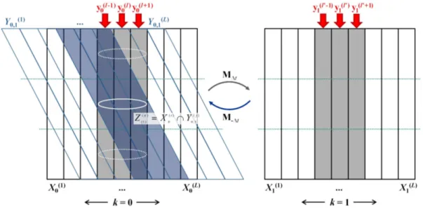
Figure 2.1: Illustration of the Kolmogorov-Sinai entropy for the first time step k= 0,1.
Xk(i)denotes the different partitions of the pseudo-phase space,y(l)k defines the observations, here column mass loadings. l andl0 state the indices of observed ash containing partitions, andM∆t andM−∆t describe the deterministic forward model and the backward in time model, respectively. The inverse image Y0,1(j) is depicted in blue. Assuming a horizontally layered structure of the ash, the white ellipses denote possible realizations of the location of the observed quantity, whereas the dotted horizontal lines indicate additional background knowledge about the partitions.
Figure 2.1 illustrates schematically the KSE for the first time step. In this work, the aim is to interrelate the theory of KSE with the information content that can be gained from volcanic ash column mass loadings from SEVIRI, which are only horizontally resolved observations. Hence, Figure 2.1 shows the different partitions of the pseudo-phase space Xk(i) arranged within columns next to each other (white and grey), at time step k = 0 on the left, and on the right at k= 1 after applying the forward model M∆t. The accuracy of the partitions can be seen as analogous to the horizontal resolution of the satellite retrieval. The grey columns picture the partitions, which include observations yk of volcanic ash content, whereas the white columns are observed to have no mass load of the observed variable. Running the backward model M−∆t starting from the phase space partitions atk = 1, the inverse imagesY0,1(i) are depicted in blue atk = 0. Within the example of volcanic ash column mass loads, the deformation of the vertical columns are taken to be caused by vertical wind shear. Looking now at the information content attained by the observations, the shaded columns all include once observed volcanic ash mass, the empty columns contain the information that no ash was observed. For a comprehensive description of the KSE, see Argyris et al. [2010].
To evaluate the information gain, the initial system state is examined. Now, let X0 be the complete set of the partitionsX0(i) andY0,1 be the set of all backward pictures Y0,1(i), such that
X0 =nX0(i);i= 1, ..., Lo, and (2.4) Y0,1 =M−∆tX1 =nY0,1(i);Y0,1(i) =M−∆tX1(i);i= 1, ..., Lo. (2.5) The intersection off all possible subsets ofX0 and Y0,1 is called first refinement of partitioning and it is defined as
Z(1) :=X0∧Y0,1 :=nZ(1)(ij);Z(1)(ij) =X0(i)∩Y0,1(j),with i, j = 1, ..., Lo. (2.6) The refinement enables a more precise localization of the initial state. Regarding the probability p(Z(1)(ij)), that a certain system state can be captured within a cell of the first partitioning refinement, the information gain is then given by
I(Z(1)) =−
L
X
i,j=1
p(Z(1)(ij)) lnp(Z(1)(ij)). (2.7) Proceeding with the application example of Figure 2.1, the information content of the volcanic ash position gained from the observations can be analyzed as follows: the areas, where white columns of X0(i) are overlaid by empty columns of Y0,1(j), have an absolute likelihood to not contain any ash, as neither at k = 0 nor at k= 1 was any ash observed. The sections that show shaded areas of X0(i) or Y0,1(j) overlapping empty columns of Y0,1(j) or X0(i), respectively, are equally probable to contain volcanic ash.
Subsequently, the regions characterized by the intersection of two shaded partitions have the highest likelihood to contain volcanic ash. Upon the hypothesis that the horizontally dotted lines display the boundaries of vertical model layers and the white ellipses describe different ensemble member realizations of the ash cloud, it becomes
2.1 Observability 13
clear that the intermediate layer is most probable to comprise the ash cloud. Thus, the location of the volcanic ash can be constrained from the full vertical column extension to the area, which is indicated by manifold observations.
Forward and backward integration over more than one time interval ∆t results in an increased refinement. Thek-th refinement is accordingly denoted as
Z(k) :=X0∧M−∆tX1∧M−2∆tX2 ∧...∧M−k∆tXk, (2.8) with the result that the total information gain of k refinements can be calculated asI(Z(k)). Longer integration times allow for better separation of the quantities in the dynamical system, such that regions of high probability emerge to be localized more precisely. In this way, correlations between the individual measurements can be identified, as the likelihood for a particular observation value depends on previous observation values. Finally, the KSEh(µ) is defined as the least upper bound of the average information gain per time unit, which is evoked by the dynamical system, with
h(µ) = sup
X,∆t k→∞lim
I(Z(k)) k∆t
!
. (2.9)
Hereby, the supremum refers to all possible partitions of the phase space X and additionally to all considered time increments ∆t. Parameter µdescribes an invariant natural probability measure, since I(Z(k)) is determined using probability density functions. In conclusion, the KSE measures the information gain per time unit one can achieve, applying a series of sequentially taken observations in combination with a model, which well characterizes the dynamical system. For regular attractors h(µ) = 0, for strange attractors h(µ) generally is > 0, whereas for random and chaotic systemsh(µ)→ ∞ for k → ∞. Due to the supremum, the computation of h(µ) is hardly achievable. Therefore, the KSE is rather utilized for a theoretical or qualitative characterization of the dynamical system.
Pesin [1977] investigated a connection between the KSE and Lyapunov exponents, so thath(µ) is numerically computable. Lyapunov exponents provide information about the stability of given trajectories in phase space, exploiting the exponential divergence or convergence of neighboring trajectories. According to Argyris et al.
[2010], the maximal Lyapunov exponent is defined as α(˜x0) = lim
k→∞sup 1
k ln |˜xk|
|˜x0|
!
, (2.10)
where ˜x0 describes the initial perturbation of the state vector x and ˜xk denotes the resulting perturbation of the reference trajectory after k time steps. Since CTMs are based on initial values that hardly match the true atmospheric state exactly, the initial deviations represent the initial value errors and uncertainties. If at least one αi >0, the model described system is called unstable, whereas negative Lyapunov exponents characterize stability and a well predictable system. As a result, it is possible to conclude how sensitive the system is to small perturbations of the initial conditions. Within a certain accuracy of observations, two initial states might not be distinguishable, although their trajectories are clearly diverse after a finite time
interval. Hence, the dynamical system acts as an information source.
Pesin [1977] found that for n-dimensional systems, Lyapunov exponents and the KSE of a subset V of the phase space are connected on certain conditions by
h(µ) =
Z
V
X+
αi(x)µ(x)dx. (2.11)
Here, the index + symbolizes that the sum only consists of positive Lyapunov exponents.
The concept of finding the most unstable initial perturbation, is considered in the theory of singular value decomposition. The emission term e of Eq. (2.2) is neglected, such that the model solution only depends on the initial condition with x(t) =M[x(t0)]. Adding small perturbations and applying a first-order Taylor series approximation, the model integration results in
M[x(t0) + ˜x(t0)] =M[x(t0)] + ∂M
∂x x(t˜ 0) +O[˜x(t0)2]. (2.12) Following Kalnay [2003], let the matrix L(t0, t) =∂M/∂x be the propagator of the tangent linear model. It is linearized at a reference trajectory x(t), which is the solution of the nonlinear model, and does not depend on ˜x(t), although it propagates the initial uncertainty to a final perturbation. Assuming the initial perturbation to be sufficiently small to evolve linearly, quadratic and higher order terms of Eq. (2.12) can be neglected. The evolution of the initial perturbation between t0 and t can be written as
˜
x(t) =L(t0, t)˜x(t0). (2.13) The model’s adjoint is equivalent to the transpose of the tangent linear modelLT and propagates the system backward in time. Singular value decomposition denotes that for the matrix L, there exist two orthogonal matricesUand V such that
UTLV =S. (2.14)
Here, UUT =Iand VVT =I, where Iis the identity matrix, and S is a diagonal matrix with the singular values σi of L as diagonal elements. The singular vectors ui and vi are the column vectors of Uand V and it can be derived that
LTLvi =σiLTui =σi2vi. (2.15) Kalnay [2003] declare vi to be the initial and ui to be the final singular vectors. The vi vectors can be determined as the eigenvectors of LLT and the squared singular values σ2i concur with the eigenvalues λi of LLT. Since vi and ui span orthonormal bases in the n-dimensional tangent linear space, they facilitate the identification of the modes, which mainly determine the linearized evolution of the system. Even if the treated system is described by differential equations with infinite degrees of freedom, the dynamic can be described by a finite number of modes by lower dimensional attractors. Accordingly, instabilities within the tangent linear model can be diagnosed as each initial singular vector component expands or contracts
![Figure 7.3: Cloud cover above Europe during the Eyjafjallajökull eruption illustrated by daily MODIS (Terra) natural color images of morning overpasses from 14 to 17 April 2010 (source: NASA [2010]).](https://thumb-eu.123doks.com/thumbv2/1library_info/3692500.1505650/72.892.120.732.660.1053/figure-europe-eyjafjallajökull-eruption-illustrated-natural-morning-overpasses.webp)