Investigation of electronic order using resonant soft x-ray diffraction
Inaugural–Dissertation zur
Erlangung des Doktorgrades
der Mathematisch–Naturwissenschaftlichen Fakult¨at der Universit¨at zu K¨oln
vorgelegt von Justina Schlappa aus Oppeln (Opole)
K¨oln 2006
Berichterstatter:
Prof. Dr. L. H. Tjeng Prof. Dr. J. R. Schneider
Vorsitzender der Pr¨ufungskomission:
Prof. Dr. L. Bohat´y
Tag der m¨undlichen Pr¨ufung: 1. Dezember 2006
Contents
Introduction 5
1 Resonant soft x-ray diffraction 9
1.1 X-ray diffraction . . . . 9
1.1.1 Geometry . . . 11
1.1.2 Structure factor . . . 12
1.1.3 Scattering volume . . . 13
1.2 Atomic form factor . . . 13
1.2.1 Isotropic terms . . . 14
1.2.2 Resonant terms . . . 15
1.3 X-ray optics . . . 16
1.3.1 Refraction . . . 17
1.3.2 Reflectivity . . . 19
1.3.3 Absorption . . . 19
1.4 Spectroscopic analysis . . . 20
2 Experimental 25 2.1 Instrumental . . . 26
2.2 Sample alignment . . . 28
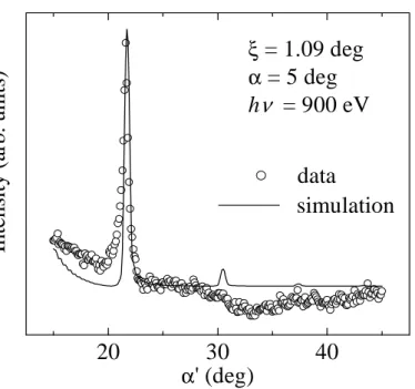
3 Diffraction from a stepped surface of SrTiO3 31 3.1 SrTiO3 . . . 32
3.2 Experimental . . . 32
3.3 Diffraction data . . . 33
3.4 Optical constants . . . 36
3.5 Modelling of the spectra . . . 42
3.6 Results and discussion . . . 44
4 Spectroscopy of stripe order in La1.8Sr0.2NiO4 47 4.1 La2−xSrxNiO4 system . . . 47
4.2 Experimental . . . 48
4.3 Bulk sensitivity . . . 50
4.4 Spectroscopic analysis . . . 52
4.4.1 Microscopic modeling . . . 55
4.5 Temperature dependence . . . 60
4.6 Discussion . . . 66 3
5 Spectroscopy of charge and orbital order in Fe3O4 67
5.1 Magnetite (Fe3O4) . . . 67
5.2 Experimental . . . 69
5.3 Diffraction data . . . 71
5.4 Spectroscopic analysis . . . 71
5.5 Conclusions . . . 75
Summary 77
Introduction
Correlated electron systems, like transition metal oxides (TMO) and rare earth (RE) systems, often display phases of spatially ordered electronic degrees of free- dom. The most known one is magnetic order, which is a periodic arrangement of magnetic moments, occurring mostly if atomic sites with partly occupied d- or f- shells are present. A non-ferromagnetic magnetic structure leads to the appearance of additional diffraction peaks (in the magnetic scattering signal), since the unit cell is effectively enlarged. This is the case for instance for various antiferromag- netic structures, including helical magnetic structures in e.g. Dy and Ho metals and multiferroic oxides and can be regarded as the formation of a superstructure with respect to the crystal lattice. Not only direction and size of magnetic moments, but also the valence or orbital occupation can be spatially modulated, leading to the formation of a long-range charge or orbital order. Systems, where such kind of orders have been predicted first are Fe3O4 (magnetite) and La1−xCaxMnO3. Both compounds are mixed-valent systems, where transition-metal ions have a formally fractional oxidation state; Fe2.5+ on octahedral sites in magnetite and Mn(3+x)+ in La1−xCaxMnO3. The occurrence of charge order has been predicted in magnetite by Verwey in 1939 [1]. He explained the sudden drop of electric conductivity in Fe3O4, when cooled below 122 K (the Verwey transition), by the occurrence of charge order, i.e., a periodic arrangement of Fe2+and Fe3+ions leading to the localization of charge carriers. Later, Goodenough demonstrated the complicated interplay between mag- netic, orbital and charge degrees of freedom for the La1−xCaxMnO3 system [2], where strong variations of magnetic properties with Ca doping were observed [3], suggesting for the first time the existence of orbital order.
Understanding of the ordering of electronic degrees of freedom is important for the study of many of the often spectacular properties in correlated systems, including high-temperature superconductivity and metal-insulator transitions. One famous example for a possible interplay between different electronic degrees of freedom is the so-called stripe order in superconducting cuprates. The strong dependence of magnetic correlation length of La2−xSrxCuO4 on doping with Sr, and above all the observation of modulation of the antiferromagnetic structure for x > 0.05 [4–7], led to the assumption of a stripe-like superstructure in the system [8–11]. In this model the doped holes form linear charge stripes in the CuO2-plane, which work as antiphase domain-walls for the antiferromagnetic order on the Cu2+-sites. The first structural evidence for the existence of such a charge-spin stripe order was found for the closely related Ni compound La2−xSrxNiO4, where mutually commensurate charge and spin modulations were observed [12–14].
While magnetic properties of a bulk material can be investigated using neutron 5
6 Introduction
diffraction, an appropriate technique for the identification of orbital and charge order was lacking for a long time. Neutrons interact directly with the atomic nuclei and with magnetic moments. Neutron diffraction is therefore the appropriate technique for investigation of crystalline and magnetic structures. However, since neutrons do not interact with electrons, they cannot reveal phenomena involving charge distribu- tion, as charge and orbital order directly, but only via effects on the crystal structure such as changed bond lengths. Therefore, superstructure reflections observed with neutrons can serve only as indication for the existence of a charge or orbital order, but cannot deliver the direct proof.
Conventional x-rays are directly sensitive to charge, but they interact with all electrons in the material in the same manner. Thus the technique is hardly sensitive to small changes involving only outer-shell electrons of heavier atoms, which are those electrons that determine the electronic properties of a solid, and the only electrons that will participate in the formation of an ordered state. The contrast created by the order may be too small, compared to the core-electrons background, to be detected. For this reason, a diffraction method is needed, which is sensitive to small changes in the configuration of valence electrons, as it is resonant x-ray diffraction.
The first attempt to study orbital order by resonant x-ray diffraction in mangan- ites was made by Murakami et al., at the Mn K-edge (1s → 4p transition) in the conventional x-ray range (6540 eV) [15, 16]. They observed a pronounced depen- dence of the scattered intensity of a ”forbidden“ reflection on the azimuthal angle of the sample, which they identified with the direct observation of orbital order.
This interpretation however received criticism from theory [17, 18], which demon- strated that diffraction studies at the Mn K-edge are not suitable to detect orbital order directly, since the method is predominantly sensitive to lattice distortions, like the accompanying collective Jahn-Teller distortion. In the following Castleton and Altarelli [19] showed that in order to probe the orbital order directly, the scattering process has to involve an excitation into a Mn 3d orbital, as is the dominant exci- tation in resonant diffraction at the Mn L2,3 edge (2p → 3d transition) in the soft x-ray range (650 eV) . The energy dependence of the scattered intensity across the resonance turns out to be so extremely sensitive to the order that no recording of the azimuthal dependence is required to identify it.
Resonant soft x-ray diffraction is therefore a method that has the potential to combine diffraction with spectroscopy. The signal is here sensitive to both; to a long-range order (structure) with a certain periodicity and to the electronic state of the TM-ions. This fact can be used to perform either spectroscopically-resolved structure study; through selecting diffraction intensity due to a certain electronic order - or to perform structurally-resolved spectroscopy study; since in combination with the appropriate microscopic model the technique is able to reveal the electronic structure of the ordered part of the system.
The first experimental study, applying resonant soft x-ray scattering at transition- metal oxides, was published in 2002 by Abbamonte et. al. [20]. Already before that, Sch¨ußler-Langeheine et al. published soft x-ray diffraction results from a single crys- talline Ho metal film at the Ho M5 resonance [21]. Experimental diffraction studies on electronic order in various transition-metal oxides followed; in manganese-oxides
Introduction 7
at the Mn L2,3 edge [22–28], copper-oxides at the Cu L2,3 and O K edge [29–31], nickel-oxides at the Ni L2,3 edge [32, 33], ruthenium-oxide at the Ru L2,3 edge [34]
and in Fe3O4 at the oxygen K edge [35]. Also the magnetic structure of thin films of Ho and Dy metals was studied at the rare earth M4,5 resonance [36–38]. Despite the fact that most of these studies use the shape of the spectra for the interpretation of their data, a full spectral analysis of the data in terms of a realistic microscopic theory - as it is state of the art in the closely related x-ray absorption spectroscopy (XAS) - is very rare, showing that the technique is still in its infant state.
This thesis deals with the application of resonant soft x-ray diffraction technique for the investigation of electronic order in transition metal oxides at the TM L2,3
edge, trying to obtain a quantitative understanding of the data. The method was therefore first systematically explored through application to a model system, with the emphasis on understanding of how x-ray optical effects have to be taken into ac- count. Two more complex systems were investigated; stripe order in La1.8Sr0.2NiO4 and charge and orbital order in Fe3O4. The main focus of the work is on the spectroscopic potential of the technique, trying to obtain a level of quantitative description of the data. For x-ray absorption spectroscopy (XAS) from transition metal oxides, cluster configuration interaction calculation provides a powerful and realistic microscopic theory. In the frame work of this thesis this cluster theory, which also considers hybridization effects between the TM-ion and the surrounding oxygen ligands, has been applied for the first time to describe resonant diffraction data; previous publications confined themselves to a pure ionic picture in their model calculations [19, 24, 25]. Results of our calculations show indeed that hybridization plays an important role for TMO, due to the strong delocalization of charges over the (TM)O6 cluster.
In the first chapter of this thesis the principles of resonant soft x-ray diffraction (RSXD) is described, including a description of the optical properties of materials for x-rays. Furthermore the spectroscopic analysis of resonant diffraction data at TML2,3 edges is explained.
The second, experimental chapter describes the experimental setups used within this thesis and gives technical details about the sample preparation.
The third chapter presents diffraction and optical data of the model systems, which were SrTiO3 single crystals with terraced surfaces. The feasibility and sen- sitivity of the technique is investigated. The optical constants are obtained across the Ti L2,3 resonance. It is shown how optical and diffraction-spectroscopy data are related in an ordered system consisting of electronically identical transition met- all ions, serving as a reference for a charge or orbitally ordered system built up of electronically inequivalent TM ions.
In the fourth chapter resonant soft x-ray diffraction data from charge and spin order in La1.8Sr0.2NiO4are presented. The existence of charge order in La1−xSrxNiO4 systems is directly confirmed. From the scattering data the spin canting and the energy splitting between the partially un-occupied eg states can be determined. A quantitative microscopic analysis of the spectral data delivers a complete picture of the electronic states involved in the stripe structure in nickelates, revealing similar- ities to cuprates, which appeared absent in XAS data [39].
8 Introduction
The fifth chapter presents the results of a resonant soft x-ray diffraction study on magnetite (Fe3O4) at the ironL2,3 edge. Two reflections are observed, (0 0 1/2) and (0 0 1). The (0 0 1/2) reflection can be clearly assigned to orbital order involving the octahedral Fe2+ sites, whereas the (0 0 1) reflection is due to charge order of the octahedral Fe2+ and Fe3+ sites.
Chapter 1
Resonant soft x-ray diffraction
Resonant soft x-ray diffraction is an experimental method combining diffraction with spectroscopy. The diffraction signal of a periodic structure is investigated, probing its energy dependence across a selected absorption edge. Due to the strong sensitivity of the spectral shape, very detailed information about the form and the electronic properties of the investigated structure can be obtained.
The energies of soft x-rays lay in the range of 200 - 2000 eV. Resonant excita- tions taking place in this region are for instance: the oxygen 1s → 2p (K edge), the transition-metal 2p →3d (L2,3 edge) and the rare-earth 3d →4f (M4,5 edge) transition. The energy range is therefore particularly suitable for investigation of transition-metal oxides and rare-earth materials, which display a rich variety of long period electronic superstructures (charge, magnetic and orbital order) match- ing the soft x-ray wavelengths [40, 41]. The structures investigated in this work were: stepped-surface SrTiO3 as a model system, charge and spin stripe-order in La1.8Sr0.2NiO4 and charge and orbital order in Fe3O4.
This chapter describes the principles of resonant soft x-ray diffraction. In the first part a few general aspects of x-ray diffraction are outlined, relevant for the technique. The second part treats the resonant interaction of x-rays with atoms. In the third part the optical properties of soft x-rays are described. The connections is made between this macroscopic reaction of matter to x-rays and the atomic picture given in part two. The last part discusses the rich information one can obtain from the spectroscopic analysis of the soft x-ray diffraction signal.
1.1 X-ray diffraction
All experiments were carried out at synchrotron-radiation sources, which provide well-focused, monochromatic and polarized photon beams of very high intensity. A monochromatic electromagnetic wave with a defined polarization direction~εcan be described, for any fixed moment in time, by the plane waveE(~r) =~ ~ε·E0·ei~k~r, where
~k is the wavevector and~rthe position vector. If such a wave hits a target potential, it can generate a non-homogeneous spherical wave, which will propagate away from the center of collision. At sufficiently large distance it will have the formf(Ω)·eikr0r. The non-scattered part of the incoming wave will be transmitted, continuing its
9
10 Resonant soft x-ray diffraction
a a
W d
k k’
q
Figure 1.1: Bragg diffraction on a set of parallel crystal planes.
propagation in the direction of incidence. The resulting wave after the scattering process can be approximated through: ψ(r) ∼ ei~k~r +f(Ω)· eikr0r. All information about the target potential is contained in the scattering amplitude f(Ω), which is a complex quantity and depends on the angle between the direction of incidence and observation Ω. The quantity accessible through the experiment is | f(Ω) |2, known as the differential cross-section. Its integration over the solid angle gives the total scattering cross-section σtot.
In a crystal the x-ray photon beam is scattered on a periodic potential, which is formed by the atomic lattice. Here each electron can be a center of collision and a source of a propagating spherical wave. The scattering amplitude of an elas- tic process involving a free electron (Thomson scattering) is equal to the classical electron radius r0 = 4πmµ0e2e = 2.82·10−5˚A , also named Thomson scattering length (me denotes here the electron mass), multiplied with a polarization factor, namely:
f(Ω) =−|ε~0†·~ε|·r0, where~εand ~ε0 represent the polarization vectors of the incoming and scattered photon (the dagger denotes the complex conjugate). The minus sign indicates that the scattering process involves a phase shift of π.
When the atomic distances in a crystal are comparable with the wavelength of x-rays, the single scattering waves can interfere constructively. Often the so-called kinematical model, which considers only interaction between the spherical parts of the waves is sufficient to describe this process, while interferences between these waves and the incident and transmitted wave are neglected. The later effects need to be included only for extremely good crystals. [42].
Constructive interference occurs when the well-known Laue-condition, or for an elastic process the equivalent Bragg’s law, is fulfilled. Both conditions can be for- mulated in terms of the so-called scattering vector~q. The scattering vector gives the momentum transfer of a photon on the crystal lattice and is defined as ~q=k~0−~k, with~k andk~0 being the wave vectors of the incident and scattered beam respectively
1.1 X-ray diffraction 11
k
k’
W
q
q
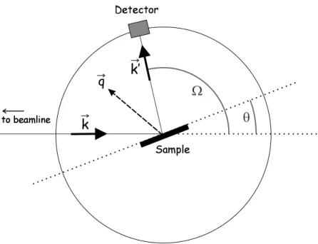
Figure 1.2: Geometry of a two-circle diffractometer.
(see Fig. 1.1 and 1.2). The Laue-condition is fulfilled when~qis equal to a reciprocal lattice vector G, so that:~ ~q=G.~
1.1.1 Geometry
Bragg diffraction is an elastic process, where the incident beam can be considered as reflected on a set of crystal planes (Fig. 1.1). For certain Bragg-angles α, the reflected waves interfere constructively. When the energy of the photons is conserved (k = k0 = 2πλ ), the absolute value of ~q is equal: q = 4πλ sin(Ω2), with Ω being the already introduced scattering angle ^(~k, ~k0). Applying the Laue condition and d being the distance between the crystal planes:
mλ= 2dsin(Ω
2), m ² N, (1.1)
This is the well-known Braggs law, here expressed in terms of the scattering angle Ω. The scattering angle is related to the Bragg-angle α (the angle between the incident/diffracted beam and the crystal plane) as follows: Ω = 2·α. The quantity Ω is directly accessible by the experiment.
The geometry used in x-ray diffraction experiments is shown in Fig. 1.2. The incident beam is fixed by the position of the beamline. To find a Bragg reflection, the sample and the detector are rotated. In the simplest set-up, there is one axis of rotation for both, the sample and detector, which is oriented perpendicularly to the direction of incidence. The angle between the incident beam and the sample surface is named θ and the angle between the incident beam and detector is exactly equal the scattering angle Ω. The scattering vector ~q points in between the direction of incidence and diffraction. The surface of the sample is placed in the center of rotation.
12 Resonant soft x-ray diffraction
1.1.2 Structure factor
The Laue or Bragg conditions give the angle, under which constructive interferences might occur. The intensity of the diffraction peak, and whether a peak is actually observed or not, depends on the structure of the unit cell of the crystal and is described in terms of the form factor fS.
The electric fields of the incident and diffracted beam are related through the scattering amplitude: Eout ∝ F · Ein. In the kinematical approximation F is a superposition of the scattering amplitudes of the single spherical waves, weighted with the appropriate phase factors. The phase relation between two coherently scattered spherical waves is given through the scattering vector ~q and the distance between their origins~r, namely: 4φ=~q·~r. Since any point in space can be chosen as the reference point, also the positions of the two points ~r1,2 can be directly used (this will have no influence on the intensity). The total scattering amplitude is then equal: f1·ei~q~r1 +f2·ei~q~r2, where f1,2 are the scattering amplitudes of the two sites.
An analogous sum can be formulated for the crystal lattice. The summation is performed over the atomic sites, the scattering amplitude of each atom being expressed through r0·f, wheref is here the atomic structure factor.
The scattering amplitude of a crystal is equal:
F =r0X
j
fj ei~q~rj
| {z }
all atoms
=r0 X
n
ei~q ~Rn
| {z }
lattice points
X
l
fl ei~q~rl
| {z }
1 unit cell
, (1.2)
The summation is performed either over all coherently scattered atoms, or by making use of the periodical structure of the crystal, first over one primitive unit cell of the crystal and then over the lattice points. The vectors ~rj in the first sum represent the positions of the atoms with respect to an origin in the crystal. In the right-hand side expression R~n represent the crystal lattice vectors and ~rl the positions of the atoms with respect to an origin in the unit cell. The Laue-condition is fulfilled when ei~q ~Rn =e2πi = 1 and:
F =N r0X
l
fl ei~q~rl ≡N r0 fS , (1.3) fS is the already mentioned structure factor, the q-dependent scattering amplitude of one unit cell and N the number of coherently scattering unit cells.
Here are some examples for the structure factor:
1. If the primitive unit cell consists of only one atom, the structure factor will be equal to the form factor f, independent on the scattering vector ~q(as long as the Laue condition applies).
2. If the unit cell consists of two atoms of the same kind, spaced half a lattice vector apart, e.g. a/2, the structure factor will be equal tofS =f(1 +ei·qa·a2).
If the component ofq along thea-direction is exactly equal 2πa, than the phase factor of the second atom will be shifted by 180 in respect to the first atom and the sum will disappear, producing no diffraction signal.
3. If the unit cell consists of two different atoms, A and B, spaced as in the example above; a/2 apart, and if againqa= 2πa, then: fS =fA+fB·ei·qa·a2 =
1.2 Atomic form factor 13
fA−fB. In this case the structure factor is equal to the difference of the two atomic form factors.
The aim of this work is the investigation not of crystal structures, but of super- structures formed within the chemical crystal structure. For the systems we inves- tigated the crystal unit cells show a periodical spacial variation of their structure factors, due e.g. to a magnetic order within the system, or generally to differences in the electronic state of the corresponding atoms. In this case the real unit cell of the crystal is effectively enlarged. Since the above notation is universal, it can be also adopted to describe the scattering amplitude of such superstructures, as well.
1.1.3 Scattering volume
According to Eq. (1.2), the diffraction amplitude is proportional to the number of coherently scattering unit cells: N = nxnynz (nx,y,z denoting the number of coherently scattering unit cells along one crystal direction). If the entire scattering volume scatters coherently, the height of a diffraction peak will grow withN2 (while the width along one direction will decrease with 1/nx,y,z). This is the case if the correlation length of the ordered system extends over the investigated scattering volume. Otherwise the peak height will be proportional to the number of domains in the volume.
In bulk samples, due to change of penetration depth of photons with energy, the scattering volume varies across the resonance. Stronger absorption leads here to a smaller N and a decrease of the diffraction signal. For non-specular geometry the probed volume depends additionally on the relation between the angle of incidence and diffraction, since the incident and diffracted beam have to cover unequal dis- tances in matter. Is θ0 ≡ Ω−θ, the angle between the diffracted beam and the sample surface, smaller than the incidence angle θ, then the path of the scattered photons in matter will be on average larger than the path for the incoming photons - and vice versa. The effective volume is proportional to [43]:
Vef f ∝ 1 σtot
sinθ0
sinθ0+ sinθ (1.4)
where σtot denotes the total scattering cross-section.
The scattering volume of thin films is limited by the sample thickness and there- fore does not change much across a resonance [38].
1.2 Atomic form factor
The atomic form factors describe the response of atoms to the electromagnetic x-ray field and depend on the kind of interaction between the electrons and photons. In a general expression they can be written as [42]:
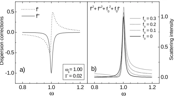
fˆ(~q, ω) = f0(~q) + ˆf0(ω) +ifˆ00(ω) (1.5) f0(~q) is an isotropic, non-resonant term. The resonant contributions; ˆf0(ω) and fˆ00(ω), also known as dispersion or anomalous corrections, are (3×3) tensors [44, 45].
14 Resonant soft x-ray diffraction
Their symmetry is given by the local symmetry at the scattering atom.
The isotropic and resonant contributions in (1.5) can be derived through solving the equation of motion of bound electrons in an alternating electromagnetic field.
The Hamiltonian of the system consists of an unperturbed term ˆH0 = ˆp2/2m+ ˆU(~r), and of interaction terms with the x-ray field, which are either linear or quadratic in the vector potential of the photon fieldA, so that: ˆ~ H = ˆH0+ ˆH1(A)+ ˆ~ H2(A~2) [46, 47].
SinceA~ is linear inc†(~k) andc(~k); the operator of photon creation and annihilation, perturbation theory yields for the scattering probability of a photon:
w=hf|H2|ii+X
m
hf|H1†|mihm|H1|ii Ei+~ω−Em
δ(Ef −Ei) (1.6)
|ii,|mi,|fi denote the initial, intermediate and final states of the electron system and Ei, Em, Ef the corresponding energies. The first order term, corresponding to the isotropic, non-resonant contribution in (1.5), is determined by the Fourier transforms of the charge and spin distribution [46]. The resonant contributions ˆf0 and ˆf00 are given by the second order terms.
1.2.1 Isotropic terms
According to Ref. [46], the first order term in (1.6) can be split into a charge and magnetic contribution. In the same way f0 in (1.5) can be separated into a charge:
fC0 and magnetic: fM0 term. The charge term is the basis of e.g. hard x-ray scattering experiments. The photons interact here with the charge density ρ(~r) at the atomic site [42]:
fC0(~q) = Z
Atom
ρ(~r)ei~q~rdr3 (1.7) The electrons are accelerated by the photon field as if they were free; like in the case of Thomson scattering. The ~q-dependence is given through the phase relations between the charges. The interaction is of a pure electric nature, and is further due in the first order to the dipole field term: E1. Without any momentum transfer (if
~q= 0), fC0 is equal to the total number of electrons on the atomic site; N =Z−V (Z ordination number and V valence). The values of fC0 for free atoms and ions are tabulated in the International Tables of Crystallography [48]. The polarization dependence of the scattering process is the same one, as for a free electron (Section 1.1): I ∝ |ε~0†·~ε|2.
The expression for the non-resonant magnetic term is analogous to (1.7), but here the density of the magnetic moments µ(~r) is considered:
fM0 (~q) = ~ω mec2
Z
Atom
µ(~r)ei~q~rdr3 (1.8) This interaction is of magnetic nature, since the spin density interacts with the magnetic field of the photon field (in the first order B1). The factor m~ωec2 (∼ 10−4) makes the scattering process very weak. The different polarization dependence from
1.2 Atomic form factor 15
charge-density scattering: I ∝ |(ε~0†×~ε)·~µ|2, provides however a way to separate the magnetic-density signal from the charge-density signal [49].
In the following; only the charge density term (fC0) will be considered when referring to f0.
1.2.2 Resonant terms
The resonant terms take into account the bounding of electrons to atoms. To under- stand their energy dependence, we look directly at the electronic state of the entire atomic site. If ψ and ϕ are two electronic states, then under the influence of an x-ray electric field a transition ψ À ϕ can be stimulated. The probability for the ψ → ϕ transition is equal to hϕ|O|ψi, with ˆˆ O being the transition operator. For resonances in the soft x-ray range, the dominating channel is the electric dipole- allowed E1 process. Therefore in the following we confine ourselves to electric dipole (E1) transitions, neglecting all other excitations, including the magnetic dipole (B1).
The electric dipole operator is defined as: ˆP =−eP
nrˆn =−eP
n(ˆxn+ ˆyn+ ˆzn), with e being the elementary charge and ˆrn the position operator for all charges in respect to the atomic nucleus. The transition probability hϕ|Pˆ|ψi corresponds to the spatial overlap of the wave functions ψ and ϕ. According to (1.6), the reso- nant diffraction term is described by a second order perturbation processes, where the atom is virtually excited into an intermediate state. In our case the occurring transition is ψ → ϕ → ψ, with ϕ being the intermediate state and ψ both; the initial and the final state. This process is coherent and therefore an observation of a Bragg-reflection is possible.
Since the functionsψ and ϕdescribe the entire electronic state of the atom, the transition probability at resonance is sensitive to both, to the charge distribution;
including the valence and orbital orientation, and to the magnetic (spin and orbital) moments at the atom [50]. This is in a clear contrast to E1-scattering outside reso- nance, where the signal is sensitive only to charge density.
The interaction between an electron and the electric part of the photon beam is given through: −e ~mA~epc , with ~p the momentum operator. If we use an adequate set of basis functions, the expression for the resonant term ˆf(ω) = ˆf0(ω) +ifˆ00(ω) becomes:
f(ω) =ˆ k2X
m
hn|Pˆt|mihm|Pˆ|ni
En+~ω−Em δ(En−Em), (1.9)
|niis the electronic ground state with energy En, ~ω the photon energy,|miare the intermediate states with energies Em and ˆPtthe inverse of the dipole operator. The summation is performed over all transition-allowed states (see Section 1.4). The expression can be also written as [51]:
f(ω) =ˆ k2hn|Pˆt 1 En+~ω−P
mHˆm+iΓˆm/2 Pˆ|ni, (1.10)
16 Resonant soft x-ray diffraction
Here ˆHm represent the Hamiltonian-operators of the intermediate states and ˆΓm the lifetime-broadening operators.
As already mentioned above, the scattering process at resonance is anisotropic.
The anisotropy is determined by the symmetry of the unoccupied atomic states, involving charge and magnetic degrees of freedom, which can be connected to / or accompanied by an anisotropy of the environment at the atomic site, e.g. due to crystal field and exchange couplings [44]. During the scattering process the polar- ization of the photon might be also changed, leading to non-diagonal elements in the transition matrix. The different anisotropy factors, and especially the charge and magnetic properties of the scattering ions, will contribute in a different way to the symmetry of ˆf(ω) [47, 50, 52–54] and can be therefore in principle separated.
The total scattering intensity of a resonant E1-process is proportional to:
I(ω, ~ε, ~ε0)∝ |ε~0†·fˆ(ω)·~ε|2 (1.11)
1.3 X-ray optics
The macroscopic optical properties of a material are described in terms of the di- mensionless refractional index n. Since the index of refraction in the x-ray regime is very close to unity, the following expression is normally used:
n= 1−δ+iβ (1.12)
The quantities δ and β are referred to as optical constants and in the conventional hard x-ray regime they are of the order 10−5 −10−8. In the soft x-ray range they can reach values up to 10−2 at resonance (Chapter 3.4). It is interesting to notice that in the hard x-ray regime - where the energy of photons lies above the most transition edges - δ is always positive, causing the real part ofn being smaller than one. In the optical regime, on the contrary, the refractional index is always larger than one, since the photon energy is lower than any transition edge.
The atomic form factors describe the response of atoms to the electromagnetic x-ray field. The scattering amplitudes in the forward scattering direction (without momentum transfer; ~q= 0) of an atomic system can be therefore used to describe the optical properties of the system at the atomic level. For a material consisting of one kind of homogeneously distributed non-magnetic atoms, with the form factor f, the refractional indexn would be [42]:
n(ω)≡1− 2πρa
k2 r0f(ω)q=0= 1− 2πρa
k2 r0{fq=00 +f0(ω) +if00(ω)} (1.13) Here ρa = ρNMA is the atomic mass density (ρ mass density, NA Avogadro-constant, M atomic mass), r0 the Thomson scattering length and k = 2πλ = ωc the wave number in vacuum. Like the scattering amplitude, the index of refraction, n, is strongly energy dependent across a resonance. For a non-isotropic system, where the optical properties are polarization-dependent, it has to be expressed through a
1.3 X-ray optics 17
a
a
n
n
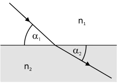
Figure 1.3: Refraction at the border of two media. When x-rays enter matter, the propagation angle becomes usually more shallow.
(3×3) tensor. δ corresponds to the real part of the scattering amplitude of the homogeneous system:
δ(ω)≡ 2πρa
k2 r0(f0+f0(ω)) (1.14) and β relates to its imaginary part:
β(ω)≡ − 2πρa
k2 r0f00(ω). (1.15)
For conventional x-rays outside resonance f0 and f00 are negligible small and thereforen is approximately equal:
n ≈1−δ ≈1− 2πρa
k2 ·r0f0. (1.16)
The index of refraction depends here only on the average number of electrons pro atomic site (or volume element), since δ ∼ N = Z − V (Z: ordination number and V: valency). The propagation direction of the x-ray beam in the material is more shallow than in vacuum, sincen is smaller than unity (the medium is optically less dense than vacuum). This leads to the occurrence of total external reflection for angles smaller than the critical angle: αc = arccos√
1−δ. In this case the electromagnetic wave cannot penetrate the second medium and the entire intensity is reflected. This effect occurs also for soft x-rays, ifδ >0.
1.3.1 Refraction
At the border of two media the propagation velocity of an electromagnetic wave changes, leading to refraction. The ratio of velocities in these media is equal to the inverse of the ratio of their refractional indices, as is known from electrodynamics [55]:
c1 c2 = λ1
λ2 = n2
n1 (1.17)
18 Resonant soft x-ray diffraction
Here λ1,2 are the corresponding wavelengths. From the continuity of the tangential component of the electric fieldE~ and its derivative across the border Snell’s law can
be deduced: cosα1
cosα2 = n2
n1 (1.18)
with α1 being the angle of incidence andα2 the angle of refraction in respect to the tangential of the surface (Fig.1.3). This notation applies if both media are isotropic and homogeneous, so thatn1,2 are position-independent scalars. If the first medium is vacuum, then n1 = 1 and n2 can be set to n. The refractional angle becomes:
cosα2 = cosα1
n (1.19)
In soft x-ray regime n is a complex number, leading to a complex cosine. To understand the meaning of the complex cosα2 we look at the wave vector of the refracted wave ei~k~r in matter. We separate ~k into contributions parallel (kk) and perpendicular (k⊥) to the tangential of the surface. Applying (1.16) and (1.18) the parallel component of ~k is equal:
kk = 2π
λ2 ·cosα2 = 2π
λ1 ·cosα1 =kkvac (1.20) and the perpendicular component:
k⊥ = 2π
λ2 ·sinα2 = 2π λ1 ·p
n2−cos2α1 (1.21) The component parallel to the surface does not change through the diffraction pro- cess, since the change of wavelength is exactly compensated by the change of the refraction angle. Only the perpendicular component k⊥ changes. If the angle of incidence is normal (α1 = 90):
k⊥= 2π λ2 = 2π
λ1 ·n=n·k⊥vac (1.22)
and~k=n·~kvac. In this case the optical constantδ defines the change in wavelength, whereas β is responsible for an exponential decrease of the electric field with depth z:
E(z) = E0·e−β·k·zei(1−δ)·k·z (1.23) For an arbitrary incidence angle, α1, since the expression in (1.20) is a square- root of a complex number, the change of the wavelength in medium will depend to some extend on the imaginary constant β and the damping of the electric field on the real constant δ. However, if the incidence angle is steep enough, the expression for k⊥ can be simplified. Since δ, β ¿ 1, their quadratic contributions in n2 might be neglected, so that: √
n2−cos2α1 ≈ p
sin2α1−2δ+ 2iβ. Now, expanding sin(α1)(1− 2(δ−iβ)sin2α1 )1/2 in the binomial series and taking into account the first two terms (valid if 2|δ+iβ|sin2α1 ¿1):
k⊥ ≈ 2π
λ1 ·sinα1− 2π λ1
δ
sinα1 +i· 2π λ1
β
sinα1 (1.24)


![Figure 3.1: Atomic force spectroscopy (AFM), stepped SrTiO 3 [M. Huijben, University of Twente].](https://thumb-eu.123doks.com/thumbv2/1library_info/3700434.1505974/33.892.311.629.148.476/figure-atomic-spectroscopy-stepped-srtio-huijben-university-twente.webp)