Fluid Dynamics

(1)

Fluid Dynamics

Prof. Huw C. Davies

WS 2005 / 2006

Version: 1.1

24^thOctober 2005

Cover:

Marine stratocumulus clouds frequently form parallel rows, or “cloud streets” along the direction of wind flow. When the flow is interrupted by an obstacle such as an island, a series of organized eddies can appear within the cloud layer downwind of the obstacle. These turbulence patterns are known as von Karman vortex streets. In this image from the June 6 2001, an impressive vortex pattern continues for over 300 km southward of Jan Mayen island. Jan Mayen is an isolated territory of Norway, located about 650 km northeast of Iceland in the north Atlantic Ocean. Jan Mayen’s Beerenberg volcano rises about 2.2 km above the ocean surface, providing a significant impediment to wind flow.

Fluid dynamicist Theodore von Karman was the first to derive the conditions under which these turbulence patterns occur. Von Karman was a professor of aeronautics at the California Institute of Technology and one of the principal founders of NASA’s Jet Propulsion Laboratory. (Source:

NASA)

Institute for Atmospheric and Climate Science

(2)

Introduction

παντ α χωρει, σνδεν µενει Heraclitus 5 cent. B. C.

1.1 Natural Flow Phenomena

Flow phenomena in natural fluid systems are pervasive and diverse. Their pervasiveness can be highlighted by noting that the range of fluid media includes: the galactic medium and interstel- lar gas; stellar and planetary atmospheres; planet Earth’s atmosphere-ocean-lake-river system;

our personal cardio-vascular system, pulmonary system, eyes, ears, larynx, alimentary canal, kidneys etc.

The diversity of documented fluid phenomena is linked to the vast range of spatial scales of the forementioned media and to the different physical processes that are active at different spatial scales. As examples of this latter point note that:

• motion in the conducting fluid regions of the Sun is influenced by, and indeed is believed to maintain, the ambient magnetic field

• the vortex like structure of large scale (∼2000 km ) cloud systems in the earth’s atmosphere is related to the earth’s rotation,

• a rapid change in the surface elevation of a mountain stream (i. e. a so-called hydraulic jump) is usually either associated with the perturbing effect of a submerged obstacle (Fig.

1.1) or is an illustration of the spontaneous transition between two flow states

• secondary circulations and eddies in rivers are often attributable to the geometry of the river bank

A fascinating and profound aspect of fluid dynamics is that there exists an unity within this diversity with different fluid media replicating similar phenomena albeit on a different scale.

Thus for example:

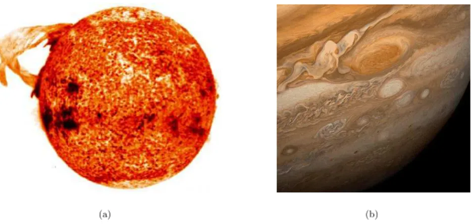
• the essence of the solar magneto-dynamo is believed to be akin to that operating in the earth’s fluid core (Fig. 1.2 (a))

• analogues of atmospheric vortex-like structures are observed in Jupiter’s atmosphere (Fig.

1.2 (b)) and in the earth’s major oceans

2 CHAPTER 1. INTRODUCTION

(a) (b)

Figure 1.1: Von Karman vortex street’s from Guadelupe, 20^th August 1999 (a) and idealized Karman street (b).

(a) (b)

Figure 1.2: A great solar helium eruption (a) was taken on December 19, 1973 using the Solar Physics Branch’s Spectroheliograph, complex flow of a dynamic atmosphere around a single spot on the planet Jupiter (b).

(5)

1.2. NATURE OF ENVIRONMENTAL FLUID DYNAMICS 3

• jump-transition phenomena also occur in galaxy-expansions, in the atmospheric Bora, in lake outflows and in the washbasin

• secondary circulations constitute a crucial component of blood flow in the aorta

1.2 Nature of Environmental Fluid Dynamics

Fluid dynamicsis the scientific study of the motion of fluids. It is founded upon the basic laws of classical physics as they apply to a fluid continuum. The mathematical formulation of these laws provides the subject with a concise, compact and well established theoretical foundation.

Nevertheless, as noted earlier, it encompasses strikingly disparate topics.

A classification of fluid dynamic studies in terms of sub-disciplines is set out in Fig. 1.3 along with examples of topics in each study-area. A fluid dynamicist would usually be involved with one particular sector of the circle. However the sectors are not independent and growth of understanding or new applications in one sector can, and often does, provide fresh insight or trigger new discoveries in other sectors.

Environmental fluid dynamicsis the sub-discipline concerned specifically with the naturally occurring phenomena of the earth’s atmosphere, oceans and enclosed water and ice systems. It embraces topics that in their spatial scale range from the global circulation of the atmosphere and ocean to the flow around and within cloud and spray droplets, and in temporal scale from that associated with air turbulence to that of glacier movement.

From an observational and experimental standpoint environmental fluid dynamics has several distinctive aspects:

• the phenomena of interest occur in natural (and often complex and inaccessible) systems in contrast to controlled laboratory conditions

• the phenomena can often be only partially (and frequently inadequately) observed

• the flow media are essentially our habitat

The general aims of the subject include determinating the structure and seeking an understanding of observed flow patterns, predicting their development and/or controlling or modifying their impact.

4 CHAPTER 1. INTRODUCTION

Figure 1.3: The fluid dynamicist’s view of the world.

1.3 Objectives of Course

The underlying aims of the course are:

• To establish the physical framework for examining environmental flow phenomena

• to develop a familiarity with the concepts of fluid dynamics

• to stimulate an awareness of the philosophy (or mode of approach) that characterizes fluid dynamic studies.

The course itself is split into three parts that provide successively:

• a concise, semi-formal (but not over-rigorous) introduction to the physical foundation and the mathematical formulation of the basic laws of fluid dynamics

• a brief overview of some of the general concepts and techniques that are common to most branches of the subject

• a sketch outline of some key ingredients of geophysical fluid dynamics

(6)

Chapter 2

Physical Foundations of Fluid Dynamics

In this sense rational mechanics will be the science of motions resulting from any forces whatso- ever, and of the forces required to produce any motions, accurately proposed and demonstrated.

Is. Newton 1686

In this section we discuss and document the physical foundations ofFluid Dynamicsand in so doing highlight the distinctive features of a fluid.

2.1 On the molecular structure of materials

First we consider the distinction between solid, liquids and gases from a micro-physical standpoint. At the corpuscular level this difference can be expressed in terms of the following factors:

• the ratio of the molecular spacing within a material relative to the equilibrium separation length (d0∼3−4·10⁻¹⁰m ),

• the strength of the intra-molecular forces, and

• the extent of the relative movement of molecules.

The strong intra-molecular forces and resultant small relative movement of molecules within a solid are consistent with a sample of solid material possessing a distinct geometric shape and being able to withstand (to a substantial degree) attempts to modify that shape (Table 2.1). In contrast the properties of liquid and gases indicate that a fluid sample would neither exhibit a preferred spatial configuration nor be able to withstand (to any degree) an attempt to distort its Table 2.1: The relationship between molecular - spacing, -forces and -movement within a solid, liquid and gas.

Molecular Intra-molecular Molecular Movement

Spacing Forces Individual Relative

solid very small strong small vibrations severely constrained

liquid ∼1 medium curved intermediate

gas very large weak piecewise linear rel. unconstrained

6 CHAPTER 2. PHYSICAL FOUNDATIONS OF FLUID DYNAMICS shape. Again the continuous movement of molecules within a fluid is associated with a perpetual transfer of momentum and heat within the fluid.

It is the mode of description and manifestation of these features on the macro-scale that we consider in the subsequent sub-sections.

2.2 The Continuum Hypothesis

Environmental fluid dynamics is usually concerned with flow phenomena that occur on the macroscopic scale, i. e. on spatial scales that are large compared with the distance between the individual molecules and on temporal scales much greater than the average time between the successive ‘molecular encounters’ of a particular molecule. On the macroscopic scale it has been proven to be appropriate to regard a fluid as a continuum i. e. to invoke a Continuum Hypothesis for the fluid medium.

In this framework physical quantities such as the mass and momentum associated with matter contained within a given ’small’ volume are assumed to be spread uniformly within that volume. The values assigned to these macroscopic quantities can be viewed as ’phase-averages’

of the mass and momentum associated with the molecules that, in reality, occupy only a small portion of that same volume. In essence the Continuum Hypothesis implies that the medium is indefinitely divisible without losing any of its defining properties and hence connotes a description of a flow system as a continuous field. Thus in the context of this Hypothesis expressions such as a point in the fluid, the density momentum and temperature at a point in the fluid, and a fluid particle are rendered meaningfull. In effect the expression the displacement of a fluid particle is not related to the displacement of some particular molecule. To avoid con- fusion and to highlight the underlying distinction between the micro- and macro-scopic frames we shall use the term fluid parcel and not fluid particle for the presumed fundamental fluid entity.

The Continuum Hypothesis provides the framework for studing fluid motion as one of the Field Theories of Classical Physics. It is important to be aware that an Hypothesis has been made, but also to recognize that one need not look far for an apologia:

• an integral aspect of the scientific approach is that of formulating a hypothesis

• in the present context a programme based upon the continuum hypothesis is eminently workable, whereas an approach based upon the laws governing elementary particles is invariably demonstrably impractical.

The programme is in effect to apply the laws of Classical Physics to a fluid medium. These laws include the principle of mass conservation, Newton’s law of motion, an equation of state and the first and second laws of Thermodynamics.

2.3 Forces acting on a fluid

In the context of the continuum hypothesis there are two kinds of forces that can act on a fluid parcel namely,

• body forces acting on the entire fluid parcel, and

(7)

2.3. FORCES ACTING ON A FLUID 7

• surface forces acting exclusively on the surface of the parcel.

We consider these two categories in turn.

1. Body Forces

These are forces that can ’act at a distance’, or in effect penetrate a fluid. Examples are the gravitational, magnetic and electrical fields. They act uniformly on the entire fluid parcel and the total force is proportional to the volume of the parcel.

i. e. Total Force =F(r, t)ρ dV,

F= the force per unit mass (it can be a function of both space and time) dV = volume of fluid parcel

In an environmental context the body force of principle interest is the gravitational field.

Newton’s law of universal gravitation states that two bodies of massM andm whose centers of mass are separated by a distancer, experience a force of attraction such that,

F=−G M m r²

r

r (2.1)

HereFis the force exerted on the body of massmdue to the gravitational pull of the body of massM, andGis the so-called gravitational constant.

The body force per unit mass on a fluid parcel in the atmosphere or ocean due to the gravitational attraction of the earth is given by

F

m≡g^∗=−G M r²

r

r (2.2)

whereMis now the mass of the earth andris essentially the radial location of the parcel.

Rewritingrin the form

r=a+z (2.3)

whereais the mean radius of the earth (If the earth’s sphericity is neglected thenzis the departure height from sea-level). It follows that

g^∗=− g

1 +^z_a² k. (2.4)

Moreover since (z/a)1 for most environmental flow systems,

g^∗≈ −gk. (2.5)

Hereg= (G M/a²)≈9.81 m s⁻²andkis in the direction of the local vertical.

2. Surface Forces

These forces can be viewed as the interaction of parcels that are juxtaposed (i. e. in ’me- chanical contact’), and expressed as the stress (i. e. force per unit area) acting on the surface of the parcel. This stress has components both normal and tangential to the surface. To define the stress, letτxyrepresent the stress components in thex-direction acting at the point 0 on the surface of a fluid parcel whose local outward normal is is in the positive

8 CHAPTER 2. PHYSICAL FOUNDATIONS OF FLUID DYNAMICS

y-direction.

It then follows that the stress is specified byτij, the components of the stress matrix,

τij=





τxx τxy τxz

τyx τyy τyz

τzx τzy τzz



 (2.6)

The surface forces in a fluid are molecular in origin and owe their existence in part to the momentum transfer accomplished by the movement and ’collision’ of molecules. We consider in turn two components of the surface stress - the pressure stress and the viscous stress.

(a) Pressure stress

A fluid exerts a normal stress even when it is stationary on the macro-scale. Consider for example a fluid confined in a container and at rest. It will nevertheless exert a

’thrust’ on the side-walls of the container due to the continual molecular bombardment of the walls. In this case the thrust will be normal to the wall since the net effect of the along wall velocity components will cancel. This normal thrust expressed as a force per unit area is the pressure (p) exerted by the fluid on the container wall. It follows that at the boundary the fluid itself experiences a stress of (−p). What is the counterpart of this thrust at a location immersed within the fluid? In effect a purely geometric plane surface within the fluid experiences an equal and opposite thrust on its two sides. More generally an arbitrary fluid parcel experiences this thrust acting normally at every point on its surface. (A proof for the non-dependence of pressure upon direction is given in Appendix I.) It follows in terms of the stress matrixτij, that for a fluid at rest,

τxx=τyy=τzz=−p(x, y, z, t). (2.7) A more vivid illustration in Fig. 2.1 is to consider a liquid of uniform densityρat rest in a gravitational field−gk. A horizontally aligned layer of width ∆zwould experience a downward force per unit length ofgρ(∆z). The fluid is at rest and thus in the absence of other forces the gravitational effect can only be offset by the difference in the pressure on the upper and lower surfaces of the stipulated layer i. e. a balance of the normal force components implies that

(p+ ∆p) +g ρ(∆z) = p , (2.8)

i. e. ∆p

∆z = −g ρ ,

and in the limit of an infinitely thin layer (i. e. ∆z → 0) we obtain the so-called hydrostatic relationship

(8)

2.3. FORCES ACTING ON A FLUID 9

z

x y

∆z

p + ∆p

p

Figure 2.1: Schematic concept of the hydrostatic relationship.

∂p

∂z=−g ρ (2.9)

Hydrostatic relationship In this particular case we have merely considered the effect of vertical variations of the pressure field upon a fluid parcel, and shown it takes the form (−∂p/∂z). In general the ’effective-stress’ associated with the pressure field is of the form

−(∇p) =− ∂p

∂xi+∂p

∂yj+∂p

∂zk

(2.10) (b) Viscous Stress

We have already noted that the continuous movement and ’collision’ of molecules within a fluid is associated with perpetual transfer of momentum and heat within a fluid. In a fluid at rest there is no net macro-scale effect. However if the fluid is in differential motion (i. e.v6= constant) or has a non-uniform temperature distribution (T6= constant) then a net flux of momentum or heat can ensue.

To illustrate this consider the idealized experimental set-up of water confined between two parallel plates (see Fig. 2.2) with the upper plate in uniform motion (u=U0) and the lower plate held fixed. It is found that (at least forU0small) a constant tangential stress (−τxz) has to be applied to keep the plate moving at this velocity and the velocity profile,u=u(z), of the flow is steady and increases linearly from zero at the base tou=U0at the top. It follows that

• the fluid establishes a force resisting the motion of the plate, and

• the stress is sustained across the entire fluid depth, so that a horizontal surface (z =z0) within the fluid experiences equal and opposite tangential stresses on its two sides. In effect the faster fluid atz=z0+tends to draw the lower slower layer along with it, whilst the lower layer acts to retard the upper layer.

The realized stress on a fluid parcel is the so-called ’viscous stress’. For a gas the stress is established almost entirely by the differential transport of momentum by

u = 0 u = U0 z

d

Figure 2.2: Idealized experiment of a moving plate between water.

upward and downward moving molecules that carry with them a value ofx-directed momentum characteristic of their layer of origin. For a liquid both this process and the modification of the intra-molecular forces by the differential motion are important.

It is appropriate to sub-divide the surface stress matrix into two components to take cognizance of the two generating mechanisms of pressure and viscous effects

i. e. let τij= −p δij

| {z } pressure

+ τij⁰

|{z}

deviatoric stress

(2.11)

where δij= 1 if i=j δij= 0 if i6=j and τxx⁰ =tau⁰yy=τzz⁰ = 0 .

Note that the (−p) is consistent with an inward directed pressure force on a fluid parcel.

The two foregoing surface forces, are related respectively to the intrinsic thermodynamic and flow properties of fluids and are considered further in the next two sub-sections.

2.4 Constitutive Relationships

Here we discuss the distinction between solids and fluids from the macrophysical/continuum standpoint. Consider the experimental set-up of Fig. 2.3 with an arbitrary material placed between the two plates, the upper plate generating a constant stressτxz=τ, and the lower plate again held fixed. The response of the material can be assessed in terms of the shear strain E=δ/d(the angle of distortion) or to the rate of strainE⁰ (the rate of change of the angle of distortion). An alternative, at least for materials that deform continuously, is to maintain a constant strain rate (ε⁰) and measure the stress (τ).

The strain response to an imposed stress (or the converse) is a property of a material’s constitution. The resulting relationship, e. g.

τ=τ(E, E⁰) or E⁰=f(τ, t) (2.12)

defines the Constitutive Equation or the Rheological equation of state. (Rheology - the science of deformation and flow of matter).

(9)

2.4. CONSTITUTIVE RELATIONSHIPS 11

τ z

d δ

Figure 2.3: Idealized experiment of a moving plate between water.

A classification of various conceivable forms of continuous media and their constitutive equations are shown in Fig. 2.5. An idealized ’Euclid Solid’ would be undistortable irrespective of magnitude ofτ, whilst for a perfectly ’Elastic Solid’ the shear strain would be purely a function ofτ(cf. Hooke’s Law for a spring states that the force is proportional to the extension). In this latter case the material would respond to a shear stress by distorting to a modified equilibrium configuration and would recover its original shape on cessation of the external stress.

At the other extreme an ideal ’Pascal Fluid’ would deform continuously (i. e.E⁰6= 0) without an associated shear stress (so thatτ /E⁰= 0) whilst for a perfectly ’Viscous Fluid’ it is the rate of shear strain (E⁰) that would be purely a function ofτ(cf. Newton’s statement in 1686 that

’the resistance arising from want of lubricity in the parts of the fluid is, other things being equal, proportional to the velocity with which the parts of the fluid are separated from one another’).

Other hybrid materials are also categorised in Fig. 2.5. For example visco-plastic substances that require the stress to exceed some threshold value before exhibiting fluid properties, and visco-elastic substances for whichE⁰=E⁰(τ, τ⁰) so that the fluid has some ’memory’ features.

stress (τ)

shear strain (E) Hookean

Non-Hookean

stress (τ)

rate of strain (E') Newtonian

Dilatant Pseudo-plastic Plastic

yield stress

Figure 2.4: Illustration of the (E,τ) and (E’,τ) profiles of the various categories.

In this course we shall concentrate almost exclusively on Newtonian Fluids. This restriction is appropriate since air and water are, to a very good approximation, Newtonian in behavior, i. e.E⁰=c τ, or equivalentτ=µ E⁰.

The second form of the constitutive relationship (τ =µ E⁰) emphasizes the fact, that al- though a fluid can not withstand (to any measure) a force that acts to distort its shape it

Perfectly Elastic Solid Ideal Euclid Solid

(τ indeterminate) Ideal Pascal Fluid

τ = 0

Fluid Solid

Perfectly Viscous Fluid

Non-Newtonian E'=f(τ) Visco-Plastic Non-Hookean

E=f(τ) Classic Hookean E=Cτ

Visco Elastic Non Bingham E'=f(τ-τ0) Bingham Body

E'=C(τ-τ0)

Classic Newtonian E'=cτ

Maxwell Fluid µE'=τ+λτ' Ideal Plastic

St. Venant-body τ=τ0

Figure 2.5: Types of continuous media.

Table 2.2: Classification of some natural media are listed below.

Material Constitutive Relationship(s) Newtonian: air, water E⁰=cτ⇒τ=µE⁰ Non-Newtonian: milk

(Pseudo-Plastic) blood

glacier-ice E⁰=Aτ³⇒τ α(E⁰)¹³ orE⁰=aτ³+bτ orτ=arcsinh(E⁰)¹³ Visco-Plastic: oceanic pack-ice E⁰=Btanh⁻¹(τ /π+ 1) (non-Bingham)

nevertheless establishes an internal stress that resists the resulting motion. The ratioµ=τ /E⁰ for a steady flow is referred to as the coefficient of viscosity of a fluid. In qualitative terms viscosity represents the property of a fluid to establish an increasing resistance to deformation for an increasing rate of deformation The molecular transport and the inter-molecular forces that contribute to viscous stress are different for different fluids and are also temperature dependent.

Thus the coefficient of viscosity (µ) varies from fluid to fluid and has a temperature dependence.

(10)

2.5. EQUATION OF STATE 13

Table 2.3: Viscosity of some common fluids.

fluid µ[ kg m⁻¹s⁻¹] ν[ m²s⁻¹] air (0^◦C) 1.70·10⁻⁵ 1.32·10⁻⁵ air (20^◦C) 1.80·10⁻⁵ 1.50·10⁻⁵ water (0^◦C) 1.80·10⁻³ 1.80·10⁻⁶ water (20^◦C) 1.00·10⁻³ 1.00·10⁻⁶ blood (37^◦C) 4.00·10⁻³

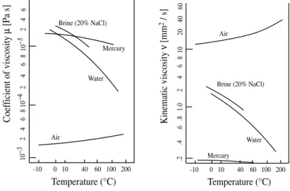
The fluid parcel acceleration to be associated with a given viscous stress would be proportional toµ/ρ(since acceleration αforce/density). Thus the value of the so-called kinematic viscosityν=µ/ρis also of interest. The values ofµandνfor air and water, displayed as a function of temperature, are given in Fig. 2.3.

Note the typical values ofµandνfor air and water at ordinary temperatures and pressure (Table 2.3 and Fig. 2.6).

Thusµair/µwater ≈ 1/60, whereas νair/νwater ≈ 14 (i. e. whenν is the relevant quantity water is in effect a much less viscous fluid than air).

-10 0 10 40 60 100 200

Temperature (°C)

10−3 2 4 6 8 10−4 2 4 6 8 10−5 2 4 6Coefficient of viscosity µ [Pa s]

Air

Water Brine (20% NaCl)

Mercury

-10 0 10 40 60 100 200

Temperature (°C)

.2 .4 .6 .8 1.0 2 4 6 8 10 20 40 60Kinematic viscosityν [mm2 / s]

Air

Water Brine (20% NaCl)

Mercury

Figure 2.6: Coefficient of viscosity (left) and kinematic viscosity (right) of common fluids.

2.5 Equation of state

The concept of the ’thermodynamic state of a fluid’ is based upon a comparison of different samples of a fluid that are in equilibrium. Two samples would be in the same ’state’ if their properties did not change upon being brought into direct contact with one another. It is usual to characterize the state of a fluid by its chemical composition, temperature and pressure. Two

14 CHAPTER 2. PHYSICAL FOUNDATIONS OF FLUID DYNAMICS samples that differed in their chemical composition and temperature would have their properties (i. e. the value of these variables) modified by diffusive processes, whilst a pressure difference would constitute an inter-sample force which would be inconsistent with the maintenance of an equilibrium state of rest. Other ’secondary’ properties of state are then defined in terms of these state variables, and in particular the equation for density is normally referred to as the Equation of State.

The atmosphere and natural water bodies are composed of a mixture of substances. Here we shall consider the Equation of State for sea water and air.

1. Sea water

contains dissolved salts (principally chloride and sodium), plankton, organic debris, dust and, near the surface, bubbles. Below the surface zone only the salts are significant and moreover their relative ratios are almost constant. In this case the chemical composition can be specified in terms of a single variable. Thus below the surface zone the equation of state for sea water takes the form

ρ=ρ(s, T, p) (2.13)

The salinity,s, is the ratio of the weight of dissolved salts to the weight of the sample of sea water (≈33-37 parts per thousand). An indication of the value ofρfor water of different salinities is displayed in Fig. 2.7 as a function of temperature. (Note that pure water has a maximum density atT ≈4^◦C - the temperature of the deeper layers of all major freshwater lakes in thermally cold atmospheric environments.)

Figure 2.7: The density of water with different salinities as a function of the temperature.

Detailed tables of the dependency ofρupons, T, and phave been compiled and are available. Some estimate of the relative importance of variations ins,T, andpcan be obtained as follows:

Consider the variations ofδρsuch that ∂ρ

ρ

≈ 1

ρ

∂ρ

∂T

p,s

dT+ 1

ρ

∂ρ

∂p

s,T

dp+ 1

ρ

∂ρ

∂s

p,T

ds

(11)

2.5. EQUATION OF STATE 15

≈ −α dT+ 1

Kdp+β ds (2.14)

whereα, βandKdenote respectively the coefficients of thermal and salinity expansions and the bulk modulus. For the normal range of values ofp, T ands(excluding the deep ocean),α≈10⁻⁴K⁻¹, K ≈10⁹N m⁻², β≈1. It is evident on assigning the typical values todT, dpanddSrespectively of≈(10 K, <10⁵N m⁻²,10⁻³), that the pressure induced variations are not significant.

For many fresh-water applications it is appropriate to approximate the equation of state to the form

ρ=ρ_∗1−α^∗θ_∗² (2.15)

whereθ_∗ = (T −T^∗), ρ_∗ = ρ_∗(T^∗) and to assign values for T^∗ (the temperature of maximum density) andα^∗, that are based upon the characteristic value of the salinity of the water body e. g. for pure waterT^∗= 4^◦C, α^∗ ≈6.8·10⁻⁶K⁻². Again for fresh water systems with comparatively small temperature variations the equation of state can be approximated by a linear relation of the form

ρ=ρ_∗ 1−α⁰θ_∗ (2.16)

2. Air

The relative proportions of the main constituents of the atmosphere are, with the exception of water vapor, comparatively constant. Thus again the composition of air is satisfactorily prescribed by specifying one variable. In this case an appropriate variable is the specific humidity (q) which describes the mass of water vapor per unit mass of air. The equation of state for air is given to a good approximation by that for an ideal gas. Thus for example for dry air

pdV = mdR T , (2.17)

i. e. pd = ρdR T ,

whereρd=md/V andR=R^∗/M= 287 J kg⁻¹K⁻¹. Here the subscriptdrefers to dry air,R^∗denotes the universal gas constant, andMthe molecular weight.

Similarly for water vapor,

e=ρvRvT (2.18)

wheree is the water vapor pressure, ρv the mass of water vapor per unit volume and Rv=R^∗/Mv.

It follows, from the partial pressure equation, that the pressurepfor moist air is given by

p = pd+e (2.19)

Note also that ρ = ρd+ρv,

so that ρd = (1−q)ρ since q=ρv

ρ It follows that:

e

p= q

ε+ (1−ε)q, where ε=Mw

Ma = R

Rv (2.20)

16 CHAPTER 2. PHYSICAL FOUNDATIONS OF FLUID DYNAMICS This is an equation that expresses the vapor pressureeof the atmosphere in terms of the specific humidityq.

Furthermore the gas equation can be rewritten in the form

ρ = p

R Tv, (2.21)

where Tv = T

1−q+q ε

is the virtual temperature.

Note that we can writeTvin the form

Tv=T(1 + 0.6078q) (2.22)

Virtual temperature

and sinceq∼O(10⁻³) it follows that for most of the atmosphere, excluding the extremely moist regions of the tropics, the approximation Tv ≈ T is appropriate. This in turn indicates that the equation of state for the atmosphere can be reasonably represented as that for an ideal gas

i. e. p=ρ R T or p α=R T with α=1

ρ (specific volume) (2.23)

Ideal gas law

(12)

Chapter 3

Mathematical Formulation of the Basic Laws

Mathematicas disciplinas, non leviter, tametsi perfunctorie attingendus esse putamus.

Huldrich Zwingli

3.1 Description of Flow

3.1.1 Coordinate Specification

The continuum hypothesis enables us to readily describe the structure of a flow field (e. g. the instantaneous velocity or density distribution). Two distinct methods are available for assigning values for these continuum variables Eulerian and Lagrangian Coordinates.

1. Eulerian Specification

This is aspace specificcoordinate frame. Flow quantities such as the velocityvor density ρare defined as functions of timetand position in spacer = (x, y, z), i. e.v=v(r, t) andρ=ρ(r, t). Thus for example the motion of the fluid in a given time interval [t] is specified completely if the velocityvis known as function of the independent variablesr andtfor all locations in the fluid medium during that time interval. In effect this specification provides a portrayal in 3D-space of the spatial flow structure at each instant in time.

2. Lagrangian Specification

This is aparcel-specificcoordinate frame. Flow quantities are defined as functions of time tand parcel location in spaceA= (a, b, c), i. e.v=v(A, t) andρ=ρ(A, t). Now the flow field is specified in terms of the location of each fluid parcel in time and space - a parcel atA0= (x0, y0, z0) at timet=t0is atAat timet, and the parcel velocity is given by v=A⁰ =dA/dt. In this reference frame the specification provides the time history of each fluid parcel.

The Lagrangian specification (which was actually proposed by Euler) is in a sense the more fundamental and has proved most insightful in certain special situations. In general however the Lagrangian specification is a cumbersome observational frame for flow exper- iments and an intractable mathematical base.

18 CHAPTER 3. MATHEMATICAL FORMULATION OF THE BASIC LAWS Here we shall adopt the Eulerian framework. However we will make extensive use of one essentially Lagrangian concept. This is the concept of the time rate of change of physical quantities associated with a fluid parcel, or the so-called material derivative.

3.1.2 The Material Derivative

The mathematical formulation of this Lagrangian concept in an Eulerian framework can be derived as follows:

Letψbe a physical quantity associated with a fluid parcel. The rate of change ofψin a fluid parcel (i. e. the advected rate of change, or the material derivative) will be denoted byDψ/Dt.

Consider a fluid element atr= (x, y, z) at a timetand moving with a velocityv= (u, v, w).

At a later timeT= (t+δt) the particle will arrive atr= (r+δr) = (X, Y, Z), whereδr= (δx, δy, δz) = (u δx, v δy, w δz).

Then Dψ

Dt = lim

δt→0

ψ(X, Y, Z, T)−ψ(x, y, z, t) δt

. (3.1)

We writeψ(X, Y, Z, T) as a Taylor series expansion aboutψ(x, y, z, t) so that

ψ(X, Y, Z, T) =ψ(x, y, z, t) + ∂ψ

∂t

u δt+ ∂ψ

∂x

u δt+ ∂ψ

∂y

v δt+ ∂ψ

∂z

w δt+· · · (3.2) It follows that

Dψ Dt =∂ψ

∂t +u∂ψ

∂x+v∂ψ

∂y+w∂ψ

∂z (3.3a)

Material derivative or equivalently

Dψ Dt =∂ψ

∂t+ (v· ∇)ψ (3.3b)

In particular note that the acceleration of a fluid parcel takes the form Dv

Dt = ∂v

∂t+ (v· ∇)v (3.4)

= ∂v

∂t−(v ∧ (∇ ∧ v)) +1

2∇(v²). (3.5)

The equivalence of the relationships in equations 3.3a / 3.3b serves to underline the mathematical distinction between the material derivative (D/Dt) and the local time derivative (∂/∂t).

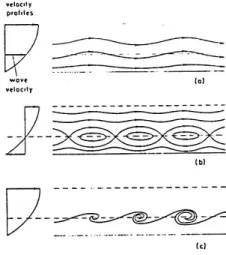
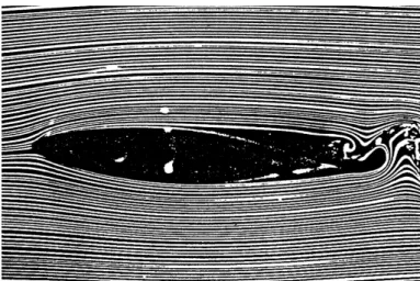
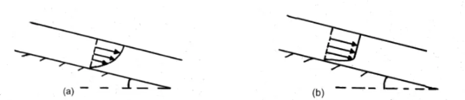
An illustration of this distinction from a physical standpoint is shown in Fig. 3.1. Hereψcon- notes the flow pattern perceived by an observer who is either stationary (panel a) or moving with the same velocity as the wave (panel b).

(13)

3.1. DESCRIPTION OF FLOW 19

Figure 3.1: Shear layer flow with traveling instability waves: (a) streamlines seen by stationary observer. (b) streamlines seen by observer traveling at the wave velocity, and (c) filament lines.

(from Hama, 1962)

3.1.3 Some Terminology Related to Flow Description

In the context of flow specification it is useful to refer to various standard ’observationally- related’ modes of flow description:

1. A parcel path(or trajectory) is the curve traced out by a fluid parcel as it moves within a fluid i. e. the path represents the Lagrangian time history of an individual parcel. It can be visualized as follows: Consider a fluid medium in which one parcel is illuminated then a long-time exposure picture would reveal the parcel path.

2. A streak line(or filament line) demarks the location of all fluid parcels that at an earlier instant in time passed through a certain point in space. It can be visualized by picturing the display formed by continually injecting a ’neutral’ dye into the flow at the chosen location.

3. A streamlineis a curve that at a given instant is everywhere tangential to the velocity vector i. e. the flow is along the streamline at the instant connsidered. It follows that the family of streamlines at a given time is defined by

dx u =dy

v =dz

w (3.6)

Streamlines

20 CHAPTER 3. MATHEMATICAL FORMULATION OF THE BASIC LAWS wherev= (u, v, w) are the flow components in a Cartesian framework (x, y, z). A short exposure photograph of a flow seeded with small, neutrally buoyant particles would reveal a pattern of streaks and the streamlines would be the series of curves tangential to these streaks.

A concept related to the streamline is that of a stream tube. It is the surface formed instantaneously by all the streamlines that pass through a given closed curve in the fluid.

3.2 Kinematics of a Flow Parcel

The velocity of a fluid usually has a continuous variation with position within the flow medium.

Thus a fluid parcel will experience a change in its geometric configuration since different portions of the parcel will move with different velocities and in different directions. It is a fundamental and informative exercise to examine the kinematic character of this geometrical change.

To facilitate the interpretation of this analysis we first restrict ourselves to two dimensional flow fields in the (x, y)-plane, and then later generalize the results to the full three-dimensional situation.

3.2.1 Case (a): Motion in a plane

Consider a fluid parcel located at pointP(x, y) with velocity components (u, v). At a neighboring locationQ(x+δx, y+δy) the associated velocity field is (u+δu), (v+δv) and can be expressed, using a Taylor series expansion, as follows

uQ = uP+ ∂u

∂x

P

δx+ ∂u

∂y

P

δy+· · · (3.7a) vQ = vP+

∂v

∂x

Pδx+ ∂v

∂y

P

δy+· · · (3.7b) In the limit ofQapproachingP, then (δu, δv) will be linear functions of (δx, δy), and only the lower order terms in the Taylor expansions need to be considered.

To illustrate the nature of the possible changes in the configuration of a small fluid element we choose to rewrite successively the equations 3.7a / 3.7b as

u =uP + 1

2 ∂u

∂x+∂v

∂y

δx+1 2

∂u

∂x−∂v

∂y

δx

P

+ 1

2 ∂u

∂y+∂v

∂x

δy−1 2

∂v

∂x−∂u

∂y

δy

P

(3.8a) v =vP +

1 2

∂u

∂x+∂v

∂y

δy−1 2

∂u

∂x−∂v

∂y

δy

P

+ 1

2 ∂u

∂y+∂v

∂x

δx+1 2

∂v

∂x−∂u

∂y

δx

P

(3.8b) The sub-division of the flow variations in the above form has a general character since D = (∂u/∂x+∂v/∂y) and ζ = (∂v/∂x−∂u/∂y) are invariant under rotation of the coordinate system, and the axes can always be aligned such that (∂u/∂y+∂v/∂x) ≡ 0 and

(14)

3.2. KINEMATICS OF A FLOW PARCEL 21

Def = (∂u/∂x−∂v/∂y)>0.

Thus we can rewrite equations 3.8a / 3.8b as

u = uP+1

2(D+ Def )δx−1

2(ζ)δy (3.9a)

v = vP+1

2(D+ Def )δy+1

2(ζ)δx (3.9b)

It follows, as we shall proceed to show, that the change in configuration of a small element is made up of the following parts

• an uniform translation with the velocity components (uP, vP),

• a volume change associated with the divergenceD,

• a shape change associated with the Deformation Def ,

• a rotation of the element associated with the vorticityζ.

The identification of these various parts can be undertaken as follows:

(a) Initial state

(b) Pure contraction

(c) Pure expansion (d) Pure deformation

(e) Vorticity

Figure 3.2: Three independent kinematic variables of divergence (b,c), deformation (d) and vorticity (e).

1. Volume Change:

Let Def ≡ζ≡0, and let the divergence be assigned values ofD=±2. Then (δu= δx, δv=δy) forD= 2 and (δu=−δx, δv=−δy) forD=−2.

22 CHAPTER 3. MATHEMATICAL FORMULATION OF THE BASIC LAWS 2. Shape Change:

LetD ≡ ζ ≡ 0 and let the deformation be assigned the value of Def = 2. Then (δu=δx, δv=−δy).

3. Rotation of Parcel:

LetD≡ Def ≡0, and let the vorticity be assigned the value ofζ= 2. Then (δu=

−δy, δv= +δx).

The foregoing sub-division of the geometrical change identifies the three independent kinematic variables of divergence, deformation and vorticity as fundamental flow variables (Fig. 3.2).

3.2.2 Case (b): Three-dimensional Motion

Proceeding as in the previous case we note that the velocity at a pointQin the immediate neighborhood of the pointPis given by,

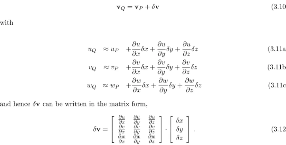
vQ=vP+δv (3.10)

with

uQ ≈uP +∂u

∂xδx+∂u

∂yδy+∂u

∂zδz (3.11a)

vQ ≈vP +∂v

∂xδx+∂v

∂yδy+∂v

∂zδz (3.11b)

wQ ≈wP +∂w

∂xδx+∂w

∂yδy+∂w

∂zδz (3.11c)

and henceδvcan be written in the matrix form,

δv=





∂u

∂x ∂u

∂y ∂u

∂z

∂v

∂x ∂v

∂y ∂v

∂z

∂w

∂x ∂w

∂y ∂w

∂z



·



 δx δy δz



 . (3.12)

Moreover the square matrix can be replaced by the sum of the associated symmetrical and antisymmetrical matrices, i. e.





∂u

∂x

∂u

∂y

∂u

∂z

∂v

∂x ∂v

∂y ∂v

∂z

∂w

∂x ∂w

∂y ∂w

∂z



=





exx exy exz

eyx eyy eyz

ezx ezy ezz



+





0 −¹2ζ ¹₂η

1

2ζ 0 −¹2ξ

−¹2η ¹₂ξ 0



 (3.13)

witheikdefined such thateik=¹₂(∂vi/∂xk+∂vk/∂xi) and the vectorωis such that

ω=∇ ∧ v= (ξ, η, ζ) (3.14)

with

ξ= ∂w

∂y −∂v

∂z

, η= ∂u

∂z−∂w

∂x

, ζ= ∂v

∂x−∂u

∂y

. (3.15)

(15)

3.3. FLOW BALANCE EQUATIONS 23

Thus

vQ= vP

|{z}

uniform translation

+ δvS

|{z}

pure straining

+ δvA

|{z}

rigid-body rotation

(3.16)

and the pure strain component can again be sub-divided into two components, i. e.

δvs= 1

3∆·



 δx δy δz





| {z }

pure isotropic expansion/contraction +





exx−¹3∆ exy exz

eyx eyy−¹3∆ eyz

ezx ezy ezz−¹3∆



·



 δx δy δz





| {z }

pure deformation

(3.17) Here ∆ =∇ ·v= (∂u/∂x+∂v/∂y+∂w/∂z), andgvcωis the vector vorticity.

3.3 Flow Balance Equations

In deriving the mathematical form for the various balance relationships we shall make extensive use of the notion of a control volume - a purely geometric volume immersed in the fluid and fixed in space.

This control volume is assumed centered atP(X, Y, Z) with side boundaries (S) of length (δx, δy, δz), mass (ρ δx δy δz), and with an associated velocityv|^p= (u, v, w).

Now consider the budget of a scalar variableAfor this control volumeV, i. e.

Net rate of accumulation = Net macro-flux ofA + Net generation ofA

ofAwithinV intoV acrossS onSor withinV

which we write symbolically as

I = II + III

The mathematical formulation for contribution I takes the form I =

∂

∂tA

δx δy δz (3.18)

To evaluate II note that the macro-flux (or flux density) ofAacross the plane boundary of the control volume located atx= (X±¹2δx) is given by

(Au)|x=X±¹2δxδy δz=

(Au)|X± ∂

∂x(Au)|X

1 2δx

δy δz . (3.19) Hence the net flux ofAintoV due to the transport across the two surfacesx= (X±¹2δx) of the control volume that are aligned perpendicular to thex-direction is,

24 CHAPTER 3. MATHEMATICAL FORMULATION OF THE BASIC LAWS

−(Au)|X+¹₂δx−(Au)|X−¹2δx

δy δz=−∂

∂x(Au)|Xδx δy δz . (3.20) Similar expressions would apply for the other pairs of surfaces ofV. It follows that the net flux ofAinto the control volume is

II =− ∂

∂x(Au) + ∂

∂y(Av) + ∂

∂z(Aw)

δx δy δz . (3.21)

Therefore the balance equation for the control volume can be written in the form, ∂

∂tA+ ∂

∂x(Au) + ∂

∂y(Av) + ∂

∂z(Aw)

δx δy δz = III (3.22) and for an arbitrary small control volume we have that

∂A

∂t + ∂

∂x(Au) + ∂

∂y(Av) + ∂

∂z(Aw)

= ∆A . (3.23)

where ∆Ais the net generation of the scalar quantityAper unit volume.

The equation 3.23 forms the core relationship for the mathematical formulation of the physical laws. In this sub-section we apply it to the principle of mass conservation (i. e. matter can neither be created nor destroyed).

Now letA=ρ, so that (A δx δy δz) refers to the mass of the control volume and ∆A≡0. Thus equation 3.23 takes the form,

∂ρ

∂t+ ∂

∂x(ρ u) + ∂

∂y(ρ v) + ∂

∂z(ρ w) = 0 (3.24)

Dρ Dt+ρ

∂u

∂x+∂v

∂y+∂w

∂z

= 0. (3.25)

In vector notation these equations are written as:

∂ρ

∂t+∇ ·(ρv) = 0 (3.26a)

Dρ

Dt+ρ(∇ ·v) = 0 (3.26b)

Continuity equation This relationship (equations 3.26a / 3.26b) is a mathematical expression for the principle of mass conservation. An alternative name that is also given to the relation is the ’Continuity Equation’.

A fluid is said to be ’effectively incompressible’ if the density of each fluid parcel remains constant i. e. Dρ

Dt= 0. (3.27)

Thus for such a fluid the mass conservation relationship reduces to

∇ ·v= 0. (3.28)

(16)

3.4. BALANCE EQUATION FOR A PASSIVE SCALAR 25 Note that for water (|Dρ/Dt|(1/ρ)) is usually extremely small, and for most natural environmental flows water can be regarded as incompressible, i. e.∇ ·v= 0.

3.4 Balance Equation for a passive Scalar

Consider for example the transport of salt in the ocean or water vapour in an unsaturated atmosphere. Letrdenote the value of the scalar per unit mass of the flow medium, so that (ρ r) denotes the amount of the scalar per unit volume.

On settingA=ρ rin equation 3.23 we have that

∂

∂t(ρ r) +∇ ·(ρ rv) = ∆(ρ r) (3.29)

The generation ∆ for a scalar comprises imposed sources/sinksQr = Qr(x, y, z, t) and the diffusion (due to molecular transport) across the surfaceS. The latter effect transfersrdown its gradient, i. e. it serves to smooth out spatial variations ofrby transferringrfrom regions of high concentration to regions of low concentration. Its form is such that

• for one dimensional variations (say in thex-direction),

∆(ρ r) = ∂

∂x

ρ Kr∂r

∂x

(3.30)

• and for a general flow configuration

∆(ρ r) =∇(ρ Kr(∇r)) (3.31)

whereKr is the coefficient of diffusivity. Note thatKr is a function of the state variables i. e.Kr=Kr(p, T, S). Typical values are shown in Table 3.1

Table 3.1: Diffusivity coefficients.

Kr fluid

1.5·10⁻⁹m²s⁻¹ for salt in water at 25^◦C 2.4·10⁻⁵m²s⁻¹ for water vapour in air at 8^◦C

Thus the balance equation for a passive scalar is

∂

∂t(ρ r) +∇ ·(ρ rv) =∇[ρ Kr(∇r)] +Qr. (3.32)

3.5 Balance Equation for Momentum

To consider the balance equation for thex, yandzcomponents of momentum we set sequentially A= (ρ u, ρ v, ρ w) in equation 3.23 and obtain for example

∂

∂t(ρ u) +∇ ·(ρ uv) = ∆(ρ u), (3.33)

26 CHAPTER 3. MATHEMATICAL FORMULATION OF THE BASIC LAWS with similar relationships forρ vandρ w.

In the case of momentum the generation terms ∆ represent the net sum of body forcesF= (F X, F Y, F X) =−gkand surface forces acting on an unit control volume. The mathematical expression for the latter forces will be derived in two steps:

1. Formulation of surface forces in terms of the stress matrix (τij)

Consider the various forces acting on the surfaces of the control volume (some of which are illustrated in Fig. 3.3).

z

x y

τ_xz + (∂τ_xz / ∂z) 0.5 δz τ_xy + (∂τ_xy / ∂y) 0.5 δy

τ_xx + (∂τ_xx / ∂x) 0.5 δx τ_xx - (∂τ_xx / ∂x) 0.5 δx

τ_xy - (∂τ_xy / ∂y) 0.5 δy τ_xz - (∂τ_xz / ∂z) 0.5 δz

Figure 3.3: Surface forces.

The net force in thex-direction due to the stresses acting on all six surfaces of the control volume is given by

SX =

τxz+ ∂

∂z(τxz)1 2δz

−

τxz− ∂

∂z(τxz)1 2δz

∂x∂y +

τxy+ ∂

∂y(τxy)1 2δy

−

τxy− ∂

∂y(τxy)1 2δy

∂x∂z +

τxx+ ∂

∂x(τxx)1 2δx

−

τxx− ∂

∂x(τxx)1 2δx

∂y∂z

= ∂

∂x(τxx) + ∂

∂y(τxy) + ∂

∂z(τxz)

∂x ∂y ∂z . (3.34)

Thus ∆(ρu), which is the net force per unit volume, is given by

∆(ρ u) =ρ(F X) + ∂

∂xτxx+ ∂

∂yτxy+ ∂

∂zτxz

, (3.35)

with similar relations for ∆(ρ v) and ∆(ρ w).

2. Formulation of the generalized constitutive relationship

It was indicated in section 2.4 that, for the simple experimental set up of Fig. 2.3 (page 11) the environmental fluids of air and water satisfy the Newtonian constitutive relationship of τ=µ E⁰=µ∂u/∂z. Here our task is to establish the generalized form of this relationship for the 3×3 components of the deviatoric stress matrixτ_ij⁰ that would apply for an arbitrary flow field and flow geometry. It has not proved possible to derive such a relationship directly from molecular theory and the procedure followed is to invoke a succesion of physically- based assumptions. These are:

(17)

3.5. BALANCE EQUATION FOR MOMENTUM 27 (a) The deviatoric stress components (τ_ij⁰) are linearly and instantaneously related to the local flow variations (i. e. the 3×3 matrix of the flow derivatives referenced in section 3.2). The ’local’ criterion is consistent with the nature of the surface stress, and the

’linearity’ and ’instantaneous’ requirements are features of a ’Newtonian’ fluid.

(b) The fluid is isotropic - i. e. there is no preferred spatial orientation. It follows that the stress components should be invariant under a reorientation of the coordinate system.

Hence we conclude from assumption (a) and section 3.2 that

τ_ij⁰ = f (∆,[deformation matrix],ω) (3.36) (c) The fluid cannot sustain internaly momentum torques. It is shown in an Appendix by a consideration of moments about axes directed through the center of the control volume that this restriction requires the matrix to be symmetric (e. g.τxy⁰ =τyx⁰ ) and hence the stress cannot be a function of the vorticity.

It can then be demonstrated that the most general form forτ_ij⁰ is,

τij⁰ =λ(∆δij) + 2µ(eij) (3.37) whereλandµare respectively the coefficient of bulk viscosity and the coefficient of shear (or dynamic) viscosity. Recall that the full stress matrix is then

τij= (−p+λ∆)δij+ 2µ(eij) (3.38) and hence

∆(ρ u) = ρ(F X)−∂p

∂x+ ∂

∂x

λ∆ + 2µ∂u

∂x

+ ∂

∂y

µ ∂u

∂y+∂v

∂x

+ ∂

∂z

µ ∂u

∂z+∂w

∂x

(3.39a)

= ρ(F X)−∂p

∂x+µ∇²u+ ∂

∂x(λ∆) +µ∂

∂x(∆) + exx∂µ

∂x+exy∂µ

∂y+exz∂µ

∂z (3.39b)

The balance equation for thex-directed momentum is given by inserting equation 3.39b into equation 3.33. For illustrative purposes we shall consider here only the limiting form of ∆(ρu) for ∆ = 0 andµ= constant (i. e. an effectively incompressible fluid of constant dynamic viscosity). In this case

∆(ρ u) =ρ(F X)−∂p

∂x+µ∇²u , (3.40)

and the balance equation for thex-directed momentum (equation 3.33) becomes

∂

∂t(ρ u) +∇ ·(ρ uv) =−∂p

∂x+µ∇²u . (3.41)

This may be rewritten, using the mass conservation relationship (equation 3.26a) in the form

ρDu

Dt = −∂p

∂x+µ∇²u (3.42)

28 CHAPTER 3. MATHEMATICAL FORMULATION OF THE BASIC LAWS

or in the from

Du Dt = −1

ρ

∂p

∂x+ν∇²u (3.43a)

Similarly the balance equations for they- andz-directed momentum can be written as Dv

Dt = −1 ρ

∂p

∂y+ν∇²v (3.43b)

Dw Dt = −1

ρ

∂p

∂z+ν∇²w−g (3.43c)

In vector notation these momentum equations 3.43a, 3.43b, 3.43c take the form:

Dv Dt =−1

ρ∇p+ν∇²v−gk (3.44)

Navier-Stokes equations

These are the so-called Navier-Stokes equations of motion.

3.6 Rotating Reference Frame

Geophysical fluid phenomena occur in media that are rotating with the earth, and their motion is usually also observed and measured in this frame of reference. However the momentum balance equation 3.44 is the form of Newton’s Law of motion applied to a fluid and applies to an inertial frame of reference, whereas a frame of reference rotating with the earth is a non-inertial frame.

Thus it is appropriate to consider the form of governing equations in an uniformly rotating reference frame. First we derive the transformed set of equations, and then seek to physically interpret the modifications to the momentum balance relationships.

LetPbe a point moving in space that is located by the vectorrrelative to a fixed originOat the timet. Let (x, y, z) be a rectangular system of coordinates which rotate aboutOwith angular velocityΩ(Fig. 3.4). In a timeδtlet the pointPmove toP⁰, whilst the position at (t+δt) of the point rigidly attached to the rotating axes, which was incident withPat timet, becomesP⁰⁰. Then

PP⁰=PP⁰⁰+P⁰⁰P⁰ (3.45)

andP⁰⁰P⁰= displacement ofPrelative to the rotating axes in the timeδt. Now, ifδΩ= angular displacement of the coordinate axes in timeδt.

Then

PP⁰=δΩ ∧ r= (Ωδt) ∧ r= (Ω ∧ r)δt (3.46)