Hausdorff and Fréchet Distance
Marc van Kreveld
1Department of Information and Computing Sciences, Utrecht University Utrecht, The Netherlands
m.j.vankreveld@uu.nl
Maarten Löffler
2Department of Information and Computing Sciences, Utrecht University Utrecht, The Netherlands
m.loffler@uu.nl
Lionov Wiratma
3Department of Information and Computing Sciences, Utrecht University Utrecht, The Netherlands
Department of Informatics, Parahyangan Catholic University Bandung, Indonesia
l.wiratma@uu.nl;lionov@unpar.ac.id
Abstract
We revisit the classical polygonal line simplification problem and study it using the Hausdorff distance and Fréchet distance. Interestingly, no previous authors studied line simplification under these measures in its pure form, namely: for a givenε >0, choose a minimum size subsequence of the vertices of the input such that the Hausdorff or Fréchet distance between the input and output polylines is at mostε.
We analyze how the well-known Douglas-Peucker and Imai-Iri simplification algorithms per- form compared to the optimum possible, also in the situation where the algorithms are given a considerably larger error threshold than ε. Furthermore, we show that computing an optimal simplification using the undirected Hausdorff distance is NP-hard. The same holds when using the directed Hausdorff distance from the input to the output polyline, whereas the reverse can be computed in polynomial time. Finally, to compute the optimal simplification from a polygonal line consisting ofnvertices under the Fréchet distance, we give anO(kn5) time algorithm that requiresO(kn2) space, wherek is the output complexity of the simplification.
2012 ACM Subject Classification Theory of computation→Computational geometry
Keywords and phrases polygonal line simplification, Hausdorff distance, Fréchet distance, Imai- Iri, Douglas-Peucker
1 Introduction
Line simplification (a.k.a. polygonal approximation) is one of the oldest and best studied applied topics in computational geometry. It was and still is studied, for example, in the context of computer graphics (after image to vector conversion), in Geographic Information Science, and in shape analysis. Among the well-known algorithms, the ones by Douglas and
1 Supported by The Netherlands Organisation for Scientfic Research on grant no. 612.001.651
2 Supported by The Netherlands Organisation for Scientfic Research on grant no. 614.001.504
3 Supported by The Ministry of Research, Technology and Higher Education of Indonesia (No.
138.41/E4.4/2015)
arXiv:1803.03550v3 [cs.CG] 27 Mar 2018
Peucker [11] and by Imai and Iri [18] hold a special place and are frequently implemented and cited. Both algorithms start with a polygonal line (henceforthpolyline) as the input, specified by a sequence of pointshp1, . . . , pni, and compute a subsequence starting with p1 and ending withpn, representing a new, simplified polyline. Both algorithms take a constant ε >0 and guarantee that the output is withinεfrom the input.
The Douglas-Peucker algorithm [11] is a simple and effective recursive procedure that keeps on adding vertices from the input polyline until the computed polyline lies within a prespecified distanceε. The procedure is a heuristic in several ways: it does not minimize the number of vertices in the output (although it performs well in practice) and it runs in O(n2) time in the worst case (although in practice it appears more like O(nlogn) time).
Hershberger and Snoeyink [17] overcame the worst-case running time bound by providing a worst-caseO(nlogn) time algorithm using techniques from computational geometry, in particular a type of dynamic convex hull.
The Imai-Iri algorithm [18] takes a different approach. It computes for every link pipj withi < j whether the sequence of verticeshpi+1, . . . , pj−1ithat lie in between in the input lie within distanceεto the segmentpipj. In this casepipj is a valid link that may be used in the output. The graphGthat has all verticesp1, . . . , pnas nodes and all valid links as edges can then be constructed, and a minimum link path from p1 to pn represents an optimal simplification. Brute-force, this algorithm runs inO(n3) time, but with the implementation of Chan and Chin [8] or Melkman and O’Rourke [21] it can be done inO(n2) time.
There are many more results in line simplification. Different error measures can be used [6], self-intersections may be avoided [10], line simplification can be studied in the streaming model [1], it can be studied for 3-dimensional polylines [5], angle constraints may be put on consecutive segments [9], there are versions that do not output a subset of the input points but other well-chosen points [16], it can be incorporated in subdivision simplification [12, 13, 16], and so on and so forth. Some optimization versions are NP- hard [12, 16]. It is beyond the scope of this paper to review the very extensive literature on line simplification.
Among the distance measures for two shapes that are used in computational geometry, theHausdorff distanceand theFréchet distanceare probably the most well-known. They are bothbottleneck measures, meaning that the distance is typically determined by a small subset of the input like a single pair of points (and the distances are not aggregated over the whole shapes). The Fréchet distance is considered a better distance measure, but it is considerably more difficult to compute because it requires us to optimize over all parametrizations of the two shapes. The Hausdorff distance between two simple polylines withnandmvertices can be computed inO((n+m) log(n+m)) time [3]. Their Fréchet distance can be computed in O(nmlog(n+m)) time [4].
Now, the Imai-Iri algorithm is considered an optimal line simplification algorithm, be- cause it minimizes the number of vertices in the output, given the restriction that the output must be a subsequence of the input. But for what measure? It is not optimal for the Haus- dorff distance, because there are simple examples where a simplification with fewer vertices can be given that still have Hausdorff distance at mostεbetween input and output. This comes from the fact that the algorithm uses the Hausdorff distance between a linkpipj and the sub-polyline hpi, . . . , pji. This is more local than the Hausdorff distance requires, and is more a Fréchet-type of criterion. But the line simplification produced by the Imai-Iri al- gorithm is also not optimal for the Fréchet distance. In particular, the input and output do not necessarily lie within Fréchet distanceε, because links are evaluated on their Hausdorff distance only.
Table 1Algorithmic results.
Douglas-Peucker Imai-Iri Optimal
Hausdorff distance O(nlogn) [17] O(n2) [8] NP-hard (this paper) Fréchet distance O(n2) (easy) O(n3) [15] O(kn5) (this paper)
The latter issue could easily be remedied: to accept links, we require the Fréchet distance between any linkpipj and the sub-polylinehpi, . . . , pjito be at mostε[2, 15]. This guaran- tees that the Fréchet distance between the input and the output is at most ε. However, it does not yield the optimal simplification within Fréchet distance ε. Because of the nature of the Imai-Iri algorithm, it requires us to match a vertex pi in the input to the vertex pi
in the output in the parametrizations, if pi is used in the output. This restriction on the parametrizations considered limits the simplification in unnecessary ways. Agarwal et al.
[2] refer to a simplification that uses the normal (unrestricted) Fréchet distance with error thresholdεas aweakε-simplification under the Fréchet distance.4 They show that the Imai- Iri algorithm using the Fréchet distance gives a simplification with no more vertices than an optimal weak (ε/4)-simplification under the Fréchet distance, where the latter need not use the input vertices.
The discussion begs the following questions: How much worse do the known algorithms and their variations perform in theory, when compared to the optimal Hausdorff and Fréchet simplifications? What if the optimal Hausdorff and Fréchet simplifications use a smaller value thanε? As mentioned, Agarwal et al. [2] give a partial answer. How efficiently can the optimal Hausdorff simplification and the optimal Fréchet simplification be computed (when using the input vertices)?
Organization and results. In Section 2 we explain the Douglas-Peucker algorithm and its Fréchet variation; the Imai-Iri algorithm has been explained already. We also show with a small example that the optimal Hausdorff simplification has fewer vertices than the Douglas- Peucker output and the Imai-Iri output, and that the same holds true for the optimal Fréchet simplification with respect to the Fréchet variants.
In Section 3 we will analyze the four algorithms and their performance with respect to an optimal Hausdorff simplification or an optimal Fréchet simplification more extensively.
In particular, we address the question how many more vertices the four algorithms need, and whether this remains the case when we use a larger value ofε but still compare to the optimization algorithms that useε.
In Section 4 we consider both the directed and undirected Hausdorff distance to compute the optimal simplification. We show that only the simplification under the directed Hausdorff distance from the output to the input polyline can be computed in polynomial time, while the rest is NP-hard to compute. In Section 5 we show that the problem can be solved in polynomial time for the Fréchet distance.
2 Preliminaries
The line simplification problem takes a maximum allowed errorεand a polylinePdefined by a sequence of pointshp1, . . . , pni, and computes a polylineQdefined byhq1, . . . , qkiand the
4 Weak refers to the situation that the vertices of the simplification can lie anywhere.
ε
p1
p2 p3
p4
p5 p6
p7
p1
p2 p3
p4
p5 p6
p7
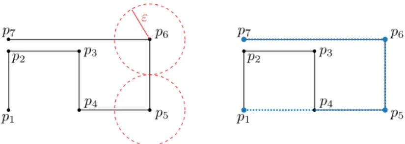
Figure 1SimplificationsIIH (same as input, left) andOPTH (in blue, right) for an example.
error is at mostε. Commonly the sequence of points definingQis a subsequence of points defining P, and furthermore,q1 =p1 and qk =pn. There are many ways to measure the distance or error of a simplification. The most common measure is a distance, denoted byε, like the Hausdorff distance or the Fréchet distance (we assume these distance measures are known). Note that the Fréchet distance is symmetric, whereas the Hausdorff distance has a symmetric and an asymmmetric version (the distance from the input to the simplification).
The Douglas-Peucker algorithm for polyline simplification is a simple recursive procedure that works as follows. Let the line segmentp1pn be the first simplification. If all points of P lie within distance ε from this line segment, then we have found our simplification.
Otherwise, letpfbe the furthest point fromp1pn, add it to the simplification, and recursively simplify the polylineshp1, . . . , pfiandhpf, . . . , pni. Then merge their simplifications (remove the duplicatepf). It is easy to see that the algorithm runs inO(n2) time, and also that one can expect a much better performance in practice. It is also straightforward to verify that polyline P has Hausdorff distance (symmetric and asymmetric) at most ε to the output.
We denote this simplification byDPH(P, ε), and will leave out the argumentsP and/orεif they are understood.
We can modify the algorithm to guarantee a Fréchet distance betweenP and its simpli- fication of at mostεby testing whether the Fréchet distance betweenP and its simplification is at mostε. If not, we still choose the most distant pointpf to be added to the simplific- ation (other choices are possible). This modification does not change the efficiency of the Douglas-Peucker algorithm asymptotically as the Fréchet distance between a line segment and a polyline can be determined in linear time. We denote this simplification byDPF(P, ε).
We have already described the Imai-Iri algorithm in the previous section. We refer to the resulting simplification asIIH(P, ε). It has a Hausdorff distance (symmetric and asymmetric) of at mostεand never has more vertices than DPH(P, ε). Similar to the Douglas-Peucker algorithm, the Imai-Iri algorithm can be modified for the Fréchet distance, leading to a simplification denoted byIIF(P, ε).
We will denote the optimal simplification using the Hausdorff distance byOPTH(P, ε), and the optimal simplification using the Fréchet distance by OPTF(P, ε). In the case of Hausdorff distance, we requireP to be withinεof its simplification, so we use the directed Hausdorff distance.
The example in Figure 1 shows thatDPH(P) and IIH(P)—which are both equal toP itself—may use more vertices than OPTH(P) = hp1, p5, p6, p7i. Similarly, the example in Figure 2 shows thatDPF andIIF may use more vertices thanOPTF.
p1
p3
p2
p4
ε
p1
p3
p2
p4
ε
Figure 2SimplificationsIIF (same as input, left) andOPTF (in blue, right) for an example.
ε
pn p1
p2
p3
pn−1
pn−2
ε
pn p1
p2
p3
pn−1
pn−2
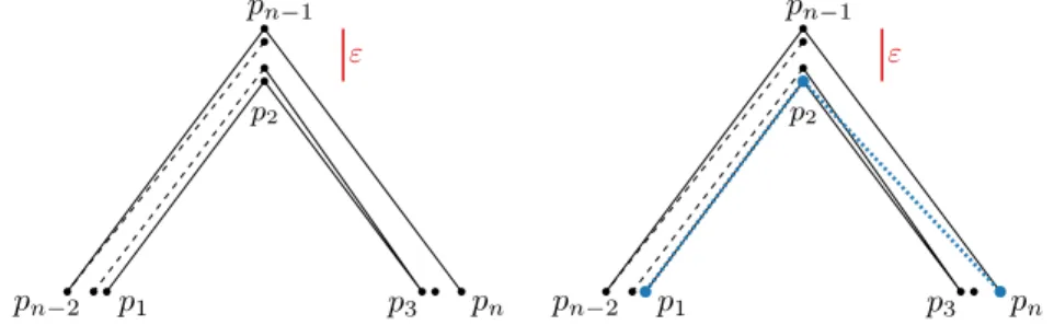
Figure 3The Douglas-Peucker and Imai-Iri algorithms may not be able to simplify at all, whereas the optimal simplification using the Hausdorff distance has just three vertices (in blue, right).
.
3 Approximation quality of Douglas-Peucker and Imai-Iri simplification
The examples of the previous section not only show thatIIH andIIF (andDPH andDPF) use more vertices thanOPTH andOPTF, respectively, they show that this is still the case if we run IIwith a larger value than ε. To letIIH use as few vertices as OPTH, we must use 2ε instead of ε when the example is stretched horizontally. For the Fréchet distance, the enlargement factor needed in the example approaches √
2 if we put p1 far to the left.
In this section we analyze how the approximation enlargement factor relates to the number of vertices in the Douglas-Peucker and Imai-Iri simplifications and the optimal ones. The interest in such results stems from the fact that the Douglas-Peucker and Imai-Iri algorithms are considerably more efficient than the computation ofOPTH andOPTF.
3.1 Hausdorff distance
To show that IIH (and DPH by consequence) may use many more vertices than OPTH, even if we enlargeε, we give a construction where this occurs. Imagine three regions with diameterεat the vertices of a sufficiently large equilateral triangle. We construct a polyline P where p1, p5, p9, . . . are in one region, p2, p4, p6, . . . are in the second region, and the remaining vertices are in the third region, see Figure 3. Letnbe such thatpn is in the third region. An optimal simplification ishp1, pi, pniwherei is any even number between 1 and n. Since the only valid links are the ones connecting two consecutive vertices ofP,IIH isP itself. If the triangle is large enough with respect toε, this remains true even if we give the Imai-Iri algorithm a much larger error threshold thanε.
ITheorem 1. For any c >1, there exists a polyline P with n vertices and anε >0 such that IIH(P, cε) hasn vertices and OPTH(P, ε)has 3vertices.
Note that the example applies both to the directed and the undirected Hausdorff distance.
ε
p1
pn−4
p4
p3
p2
pn−3 pn−2
pn−1 pn p1
pn−4
p4
p3
p2
pn−3 pn−2
pn−1 pn
pn−5
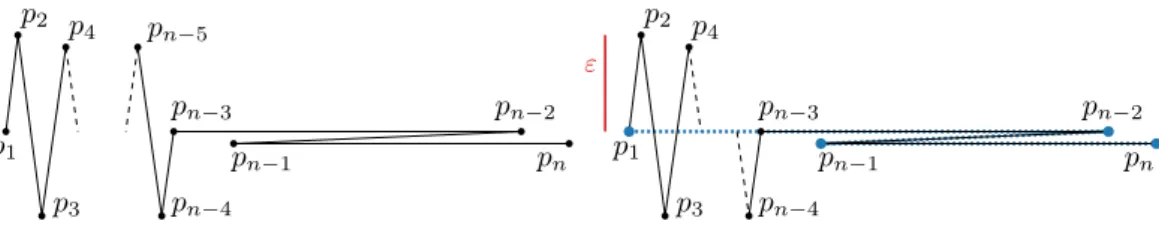
Figure 4Left: a polyline on which the Fréchet version of the Douglas-Peucker algorithm performs poorly and the output polyline containsnvertices. Right: the optimal simplification contains four vertices (in blue).
3.2 Fréchet distance
Our results are somewhat different for the Fréchet distance; we need to make a distinction betweenDPF andIIF.
Douglas-Peucker We construct an example that shows thatDPF may have many more vertices than OPTF, even if we enlarge the error threshold. It is illustrated in Figure 4.
Vertexp2is placed slightly higher thanp4, p6, . . .so that it will be added first by the Fréchet version of the Douglas-Peucker algorithm. Eventually all vertices will be chosen. OPTF
has only four vertices. Since the zigzag pn−3, . . . , pn can be arbitrarily much larger than the height of the vertical zigzag p1, . . . , pn−4, the situation remains if we make the error threshold arbitrarily much larger.
ITheorem 2. For anyc >1, there exists a polyline P withn vertices and an ε >0 such that DPF(P, cε) hasn vertices and OPTF(P, ε)has 4 vertices.
Remark One could argue that the choice of adding the furthest vertex is not suitable when using the Fréchet distance, because we may not be adding the vertex (or vertices) that are to “blame” for the high Fréchet distance. However, finding the vertex that improves the Fréchet distance most is computationally expensive, defeating the purpose of this simple algorithm. Furthermore, we can observe that also in the Hausdorff version, the Douglas- Peucker algorithm does not choose the vertex that improves the Hausdorff distance most (it may even increase when adding an extra vertex).
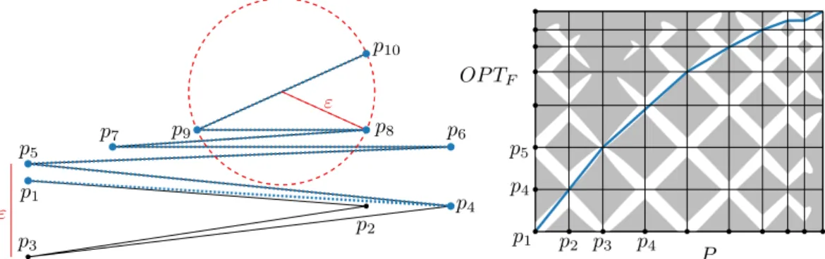
Imai-Iri Finally we compare the Fréchet version of the Imai-Iri algorithm to the optimal Fréchet distance simplification. Our main construction has ten vertices placed in such a way thatIIF has all ten vertices, while OPTF has only eight of them, see Figures 5 and 6.
It is easy to see that under the Fréchet distance,IIF =OPTF for the previous construc- tion in Figure 4. We give another input polylineP in Figure 6 to show thatIIF also does not approximateOPTF even ifIIF is allowed to useεthat is larger by a constant factor.
We can append multiple copies of this construction together with a suitable connection in between. This way we obtain:
ITheorem 3. There exist constants c1 >1, c2 >1, a polyline P with n vertices, and an ε >0 such that |IIF(P, c1ε)|> c2|OPTF(P, ε)|.
By the aforementioned result of Agarwal et al. [2], we know that the theorem is not true forc1≥4.
ε p1
p3
p4 p10
p9 p8 p6
p5 p7
p2
Figure 5 The Imai-Iri simplification will have all vertices because the only valid links with a Fréchet distance at mostεare the ones connecting two consecutive vertices in the polyline.
ε
ε p1
p3
p4 p10
p9 p8 p6
p5
p7
p2
P OP TF
p1
p4
p2 p3
p5
p4
Figure 6The optimal simplification can skipp2 andp3; in the parametrizations witnessing the Fréchet distance, OPTF “stays two vertices behind” on the input until the end. Right, the free space diagram ofP andOPTF.
4 Algorithmic complexity of the Hausdorff distance
The results in the previous section show that both the Douglas-Peucker and the Imai-Iri algorithm do not produce an optimal polyline that minimizes the Hausdorff or Fréchet dis- tance, or even approximate them within any constant factor. Naturally, this leads us to the following question: Is it possible to compute the optimal Hausdorff or Fréchet simplification in polynomial time?
In this section, we present a construction which proves that under the Hausdorff distance, computing the optimal simplified polyline is NP-hard.
4.1 Undirected Hausdorff distance
We first consider the undirected (or bidirectional) Hausdorff distance; that is, we require both the maximum distance from the initial polylineP to the simplified polylineQand the maximum distance fromQtoP to be at mostε.
ITheorem 4. Given a polylineP =hp1, p2, . . . , pniand a valueε, the problem of computing a minimum length subsequence QofP such that the undirected Hausdorff distance between P andQis at most εis NP-hard.
We prove the theorem with a reduction from Hamiltonian cycle in segment intersection graphs. It is well-known that Hamiltonian cycle is NP-complete in planar graphs [14], and by Chalopin and Gonçalves’ proof [7] of Scheinerman’s conjecture [22] that the planar graphs
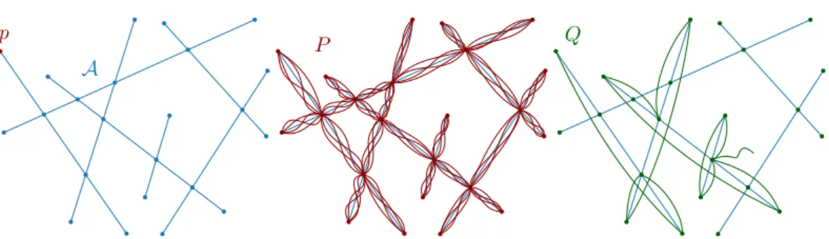
p P
A
Q
Figure 7 The construction: A is the arrangement of a set of segments S. We build an input pathP that “paints” overS completely, and we are looking for an output pathQthat corresponds to a Hamiltonian cycle. In this case, there is no Hamiltonian cycle, and the path gets stuck.
are included in the segment intersections graphs it follows that Hamiltonian cycle in segment intersections graphs is NP-complete.
LetS be a set ofn line segments in the plane, and assume all intersections are proper (if not, extend the segments slightly). LetGbe its intersection graph (i.e. Ghas a vertex for every segment inS, and two vertices in Gare connected by an edge when their corres- ponding segments intersect). We assume thatGis connected; otherwise, clearly there is no Hamiltonian cycle inG.
We first construct an initial polylinePas follows. (Figure 7 illustrates the construction.) Let A be the arrangement ofS, let pbe some endpoint of a segment in S, and let π be any path onAthat starts and finishes atpand visits all vertices and edges ofA(clearly,π may reuse vertices and edges). ThenP is simply 3n+ 1 copies ofπappended to each other.
Consequently, the order of vertices inQnow must follow the order of these copies. We now setεto a sufficiently small value.
Now, an output polyline Q with Hausdorff distance at mostε to P must also visit all vertices and edges ofA, and stay close toA. Ifεis sufficiently small, there will be no benefit forQto ever leaveA.
ILemma 5. A solutionQof length3n+1exists if and only ifGadmits a Hamiltonian cycle.
Proof. Clearly, any simplificationQwill need to visit the 2nendpoints of the segments in S, and since it starts and ends at the same pointp, will need to have length at least 2n+ 1.
Furthermore, Q will need to have at least two internal vertices on every segment s ∈ S:
once to enter the segment and once to leave it (note that we cannot enter or leave a segment at an endpoint since all intersections are proper intersections). This means the minimum number of vertices possible forQis 3n+ 1.
Now, ifGadmits a Hamiltonian cycle, it is easy to construct a simplification with 3n+ 1 vertices as follows. We start atpand collect the other endpoint of the segments1 of which pis an endpoint. Then we follow the Hamiltonian cycle to segment s2; by definitions1s2 is an edge inGso their corresponding segments intersect, and we use the intersection point to leaves1 and enters2. We proceed in this fashion until we reachsn, which intersects s1, and finally return top.
On the other hand, any solution with 3n+ 1 vertices must necessarily be of this form and therefore imply a Hamiltonian cycle: in order to have only 3 vertices per segment the vertex at which we leaves1 must coincide with the vertex at which we enter some other segment, which we calls2, and we must continue until we visited all segments and return top. J
4.2 Directed Hausdorff distance: P → Q
We now shift our attention to the directed Hausdorff distance fromP to Q: we require the maximum distance fromP toQ to be at most ε, but Qmay have a larger distance to P.
The previous reduction does not seem to work because there is always a Hamiltonian Cycle of length 2nfor this measure. Therefore, we prove the NP-hardness differently.
The idea is to reduce from Covering Points By Lines, which is known to be both NP-hard [20] and APX-hard [19]: given a setS of points inR2, find the minimum number of lines needed to cover the points.
Let S = {s1, . . . , sn} be an instance of the Covering Points By Lines problem.
We fix ε based onS and present the construction of a polyline connecting a sequence of m= poly(n) points: P =hp1, p2, ..., pmisuch that for every 1≤i≤n, we havesi=pj for some 1≤j ≤m. The idea is to force the simplification Qto cover all points in P except those inS, such that in order for the final simplification to cover all points, we only need to collect the points in S using as few line segments as possible. To this end, we will place a number offorced pointsF ⊂P, where a pointf isforcedwhenever its distance to any line through any pair of points in P is larger thanε. Since Qmust be defined by a subset of points inP, we will never coverf unless we choose f to be a vertex ofQ. Figure 8 shows this idea. On the other hand, we need to place points that allow us to freely draw every line through two or more points in S. We create two point sets L and R to the left and right of S, such that for every line through two of more points inS, there are a point inL and a point inR on that line. Finally, we need to build additional scaffolding around the construction to connect and cover the points in LandR. Figure 9 shows the idea.
We now treat the construction in detail, divided into three parts with different purposes:
1. a sub-polyline that contains S;
2. a sub-polyline that contains LandR; and
3. two disconnected sub-polylines which share the same purpose: to guarantee that all vertices in the previous sub-polyline are themselves covered byQ.
Part 1: Placing S
First, we assume that every point inS has a uniquex-coordinate; if this is not the case, we rotate S until it is.5 We also assume that every line through at least two points of S has a slope between −1 and +1; if this is not the case, we vertically scale S until it is. Now, we fixε to be smaller than half the minimum difference between any twox-coordinates of points in S, and smaller than the distance from any line through two points in S to any other point inS not on the line.
We place n+ 1 forced points f1, f2, ..., fn, fn+1 such that the x-coordinate of fi lies between thex-coordinates ofsi−1 and si and the points lie alternatingly above and below S; we place them such that the distance of the line segment fifi+1 to si is 32ε and the distance of fifi+1 to si−1 is larger than ε. Next, we place two auxiliary points t+i and t−i on fifi+1 such that the distance of each point to si is 2ε; refer to Figure 8. Then letτ1 =hf1, t+1, s1, t−1, f2, t−2, s2, t+2, f3, . . . , fn+1i be a polyline connecting all points in the construction;τ1 will be part of the input segmentP.
The idea here is that all forced points must appear on Q, and if only the forced points appear onQ, everything in the construction will be coveredexceptthe points inS(and some
5 Note that, by nature of theCovering Points By Linesproblem, we cannot assumeS is in general position; however, a rotation for which allx-coordinates are unique always exists.
s2
s3 s1
f1
t+1 t−1
f2 f3
f4
Figure 8 Example of τ1 where n= 3.
For a given ε, the (simplified) polyline f1, f2, f3, f4covers the gray area but not the blue pointss1, s2, s3.
s2 s3
s1
u`1 ur1
u`2 ur2
R1
L2
L1
ε
v1r v`1
l1
l2
l3
r1
r2
r3 R2
Figure 9 Construction to allow the lines that can be used to cover the points ofS. To ensure the order of vertices inQ, we create copies of L and R. Then, Qcan use them alternatingly.
arbitrarily short stubs of edges connecting them to the auxiliary points). Of course, we could choose to include more points inτ1 in Qto collect some points of S already. However, this would cost an additional three vertices per collected point (note that using fewer than three, we would miss an auxiliary point instead), and in the remainder of the construction we will make sure that it is cheaper to collect the points inS separately later.
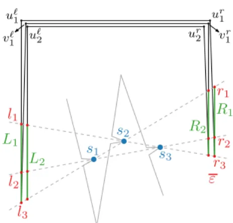
Part 2: Placing and covering L and R
In the second part of the construction we create two sets ofO(n2) vertices,LandR, which can be used to make links that coverS. Consider the set Λ of allk≤n22−n unique lines that pass through at least two points inS. We create two sets ofkpointsL={l1, l2, . . . , lk}and R={r1, r2, . . . , rk} with the following properties:
the line throughli andri is one of theklines in Λ,
the line throughli andrj fori6=j has distance more thanεto any point inS, and the points inL(resp. R) all lie on a common vertical line.
Clearly, we can satisfy these properties by placingLandRsufficiently far fromS. We create a vertical polyline for each set, which consists ofk−1 non-overlapping line segments that are connecting consecutive vertices in theiry-order from top to bottom. LetR1 andL1be such polylines containingk vertices each.
Now, each line that covers a subset ofS can become part ofQ by selecting the correct pair of vertices fromR and L. However, if we want Q to contain multiple such lines, this will not necessarily be possible anymore, since the order in which we visitR1andL1is fixed (and to create a line, we must skip all intermediate vertices). The solution is to make h copies6R1, R2, . . . , Rh ofR1andhcopiesL1, L2, . . . , LhofL1and visit them alternatingly.
Here h = dn2e is the maximum number of lines necessary to cover all points in S in the Covering Points By Linesproblem.
6 The copies are in exactly the same location. If the reader does not like that and feels that points ought to be distinct, she may imagine shifting each copy by a sufficiently small distance (smaller thanε/h) without impacting the construction.
g e
z
g e
z
τ1
τ2 τ2 τ1
Figure 10Schematic views of connecting up different parts of the NP hardness construction into a single polyline. The bold polylines showτ1andτ2and indicate multiple parts ofP close together.
We create a polyline τ2 that contains R1 and L1 by connecting them with two new verticesur1 andu`1. Bothur1andu`1should be located far enough fromR1andL1 such that a link between ur1 and a vertex in L1 (and u`1 with R1) will not cover any point inS. To ensure that the construction ends at the last vertex inLh, we use two verticesv`1andv1r, see Figure 9. Let τ2 =hR1, ur1, u`1, L1, v`1, vr1, R2, ur2, u`2, L2, v`2, . . . , Lhibe a polyline connecting all points in the construction;τ2 will also be part of the inputP.
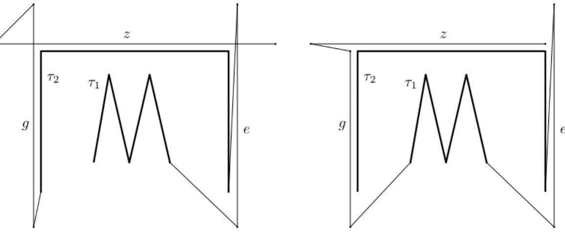
Part 3: Putting it together
All vertices inτ1can be covered by the simplificationhf1, f2, ..., fn+1iand a suitable choice of links inτ2. Therefore, the last part is a polyline that will definitely cover all vertices in τ2and at the same time, serve as a proper connection betweenτ1andτ2. Consequently, all vertices in this part will also beforcedand therefore be a part of the final simplified polyline.
We divide this last part into two disconnected polylines: τ3a and τ3b. The main part of τ3ais a vertical line segmentethat is parallel toR1. There is a restriction toe: the Hausdorff distance from each ofRi, uri, vjr(1≤j < i≤h), and also from line segments between them toeshould not be larger than ε. In order to forceeto be a part of the simplified polyline, we must place its endpoints away fromτ2. Then,τ1 andτ2 can be connected by connecting fn+1∈τ1 and the first vertex inR1 to different endpoints ofe.
Next, the rest ofτ2 that has not been covered yet, will be covered byτ3b. First, we have a vertical line segment g that is similar to e, in order to cover Li, u`i, v`j (1 ≤j < i ≤h), and all line segments between them. Then, a horizontal line segment z is needed to cover all horizontal line segmentsuriu`i andv`jvjr (1≤j < i≤h). Similar toe, the endpoints of g andzshould be located far fromτ2, implying thatzintersects botheandg. This is shown in Figure 10, left. We complete the construction by connecting the upper endpoint ofg to the left endpoint ofz and the lower endpoint ofg to the last vertex inLh.
We can show that even if the input is restricted to be non-self-intersecting, the simpli- fication problem is still NP-hard. We modify the last part of the construction to remove the three intersections. Firstly, we shorten z on the right side and place it very close to ur1. Since the right endpoint of z is an endpoint of the input, it will always be included in a simplification. Secondly, to remove the intersection of g and z, we bring the upper endpoint of g to just below z, so very close to u`1. To make sure that we must include g in the simplification we connect the lower endpoint of g to f1. This connecting segment is
further fromg so it cannot help enough to cover the lower part ofg; only g itself can do that. This is shown in Figure 10, right.
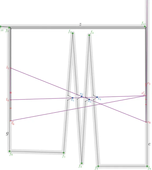
We present a full construction ofP =hτ3b, τ1, τ3a, τ2iforn= 4 in Figure 11.
ITheorem 6. Given a polylineP =hp1, p2, . . . , pniand a valueε, the problem of computing a minimum length subsequenceQof P such that the directed Hausdorff distance from P to Qis at mostεis NP-hard.
Proof. The construction containsO(n2) vertices and a part of its simplified polyline with a constant number of vertices that containsf1, f2, ..., fn+1 and all vertices inτ3a andτ3b can cover all vertices in the construction except forS. Then, the other part of the simplified polyline depends on links to cover points in S. These links alternate between going from left to right and from right to left. Between two such links, we will have exactly two vertices from someLor two from some R.
The only two ways a point si can be covered is by including si explicitly or by one of theO(n) links that cover si and at least another point sj. If we includesi explicitly then we must also include t+i and t−i or else they are not covered. It is clearly more efficient (requiring fewer vertices in the simplification) if we use a link that coverssiand anothersj, even ifsj is covered by another such link too. The links of this type in an optimal simplified polyline correspond precisely to a minimum set of lines coverings1, . . . , sn. Therefore, the simplified polyline of the construction contains a solution toCovering Points By Lines instance. SinceP in the construction is simple, the theorem holds even for simple input. J
4.3 Directed Hausdorff distance: Q → P
Finally, we finish this section with a note on the reverse problem: we want to only bound the directed Hausdorff distance fromQto P (we want the output segment to stay close to the input segment, but we do not need to be close to all parts of the input). This problem seems more esoteric but we include it for completeness. In this case, a polynomial time algorithm (reminiscent of Imai-Iri) optimally solves the problem.
ITheorem 7. Given a polylineP =hp1, p2, . . . , pniand a valueε, the problem of computing a minimum length subsequenceQof P such that the directed Hausdorff distance from Qto P is at mostεcan be solved in polynomial time.
Proof. We compute the region with distanceεfromP explicitly. For every link we compute if it lies within that region, and if so, add it as an edge to a graph. Then we find a minimum link path in this graph. For a possibly self-intersecting polyline as the input a simple algorithm takesO(n4) time (faster is possible). J
5 Algorithmic complexity of the Fréchet distance
In this section, we show that for a given polyline P = hp1, p2, ..., pni and an error ε, the optimal simplificationQ=OPTF(P, ε) can be computed in polynomial time using a dynamic programming approach.
5.1 Observations
Note that a link pipj in Qis not necessarily within Fréchet distance ε to the sub-polyline hpi, pi+1, ..., pji(for example, p1p3 in Figure 2). Furthermore, a (sequence of) link(s) inQ could be mapped to an arbitrary subcurve of P, not necessarily starting or ending at a
f1
f5
s1 s4
f6
f7
f8
f9
f10
f11
r1
r03 l4
r6 l1
s3
s2
f3
f2 f4
e g
z
l60
Figure 11The full construction showing that computingOPTHis NP-hard.τ3ais a line segment e=f6, f7 andτ3b=hf8, ..., f11i. The endpoints of the construction aref11 andl06∈L2. The gray area is withinε from the sub-polyline consist of all green vertices: hf11, .., f8, f1, .., f7i, which is a part of the simplification. The rest of the simplification is the purple polylinehf7, r6, l1, l4, r30, l06i that covers all blue pointsS (r30 ∈R2 andl06∈L2). In order to show the red points clearly,εused in this figure is larger than it needs to be. Consequently, a links1s4 can covers2 ands3, which is not possible ifεis considerably smaller.
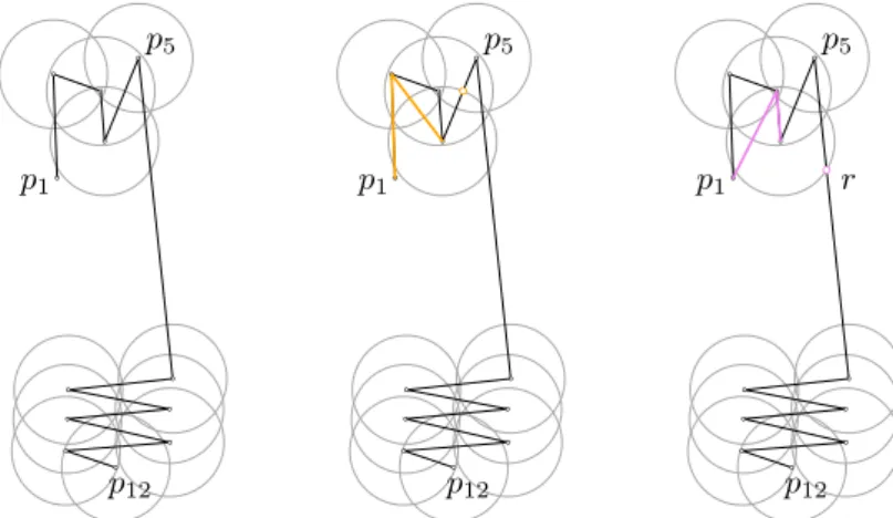
p1 p1 p1
p5 p5 p5
p12 p12 p12
r
Figure 12 An example where the farthest-reaching simplification up top4 using 2 links is not part of any solution that usesp4. Left: the input curvePin black, with circles of radiusεaround all vertices in light gray. Middle: A 2-link simplification ofhp1, p2, p3, p4ithat reaches up to a point on p4p5(in yellow) which can be extended to a 4-link simplification ofP. Right: A 2-link simplification ofhp1, p2, p3, p4ithat reaches pointronp5p6 (in pink) which does not allow simplification.
vertex ofP. For example, in Figure 6, the sub-polylinehp1, p4, p5, p6i has Fréchet distance εto a sub-polyline of P that starts atp1 but ends somewhere between p4 andp5. At this point, one might imagine a dynamic programming algorithm which stores, for each vertex pi and valuek, the pointp(i, k) on P which is the farthest alongP such that there exists a simplification of the part ofP up topi usingk links that has Fréchet distance at mostε to the part ofP up top(i, k). However, the following lemma shows that even this does not yield optimality; its proof is the example in Figure 12.
ILemma 8.There exists a polylineP =hp1, . . . , p12iand an optimalε-Fréchet-simplification that has to usep4,Q=hp1, p2, p4, p5, p12i using4 links, with the following properties:
There exists a partial simplificationR=hp1, p3, p4iofhp1, . . . , p4iand a pointronp5p6 such that the Fréchet distance between Rand the subcurve ofP up tor is≤ε, but there exists no partial simplification S of hp4, . . . , p12i that is within Fréchet distance ε to the subcurve ofP starting atr that uses fewer than7 links.
5.2 A dynamic programming algorithm
Lemma 8 shows that storing a single data point for each vertex and value ofkis not sufficient to ensure that we find an optimal solution. Instead, we argue that if we maintain the set ofallpoints at P that can be “reached” by a simplification up to each vertex, then we can make dynamic programming work. We now make this precise and argue that the complexity of these sets of reachable points is never worse than linear.
First, we define π, a parameterization of P as a continuous mapping: π : [0,1]→ R2 whereπ(0) =p1 andπ(1) =pn. We also writeP[s, t] for 0≤s≤t≤1 to be the subcurve ofP starting atπ(s) and ending atπ(t), also writingP[t] =P[0, t] for short.
We say that a point π(t) can be reachedby a (k, i)-simplification for 0≤k < i≤n if there exists a simplification ofhp1, . . . , piiusingklinks which has Fréchet distance at most εto P[t]. We letρ(k, i, t) =true in this case, and falseotherwise. With slight abuse of notation we also say thattitself is reachable, and that an intervalIis reachable if allt∈I are reachable (by a (k, i)-simplification).
IObervation 1. A point π(t) can be reached by a (k, i)-simplification if and only if there exist a 0< h < iand a 0≤s≤tsuch thatπ(s) can be reached by a (k−1, h)-simplification and the segmentphpi has Fréchet distance at mostεtoP[s, t].
Proof. Follows directly from the definition of the Fréchet distance. J Observation 1 immediately suggests a dynamic programming algorithm: for everykand iwe store a subdivision of [0,1] into intervals whereρis true and intervals whereρis false, and we calculate the subdivisions for increasing values of k. We simply iterate over all possible values of h, calculate which intervals can be reached using a simplification via h, and then take the union over all those intervals. For this, the only unclear part is how to calculate these intervals.
We argue that, for any givenkandi, there are at mostn−1 reachable intervals on [0,1], each contained in an edge ofP. Indeed, every (k, i)-reachable pointπ(t) must have distance at mostε to pi, and since the edgee ofP that π(t) lies on intersects the disk of radiusε centered at pi in a line segment, every point on this segment is also (k, i)-reachable. We denote the farthest point onewhich is (k, i)-reachable by ˆt.
Furthermore, we argue that for each edge ofP, we only need to take the farthest reachable point into account during our dynamic programming algorithm.
ILemma 9. If k,h,i,s, and t exist such thatρ(k−1, h, s) =ρ(k, i, t) =true, and phpi has Fréchet distance≤ε toP[s, t], thenphpi also has Fréchet distance≤ε toP[ˆs,ˆt].
Proof. By the above argument,P[s,s] is a line segment that lies completely within distanceˆ εfromph, andP[t,ˆt] is a line segment that lies completely within distanceεfrompi.
We are given that the Fréchet distance betweenphpi andP[s, t] is at mostε; this means a mapping f : [s, t] → phpi exists such that |π(x)−f(x)| ≤ ε. Let q = f(s0). Then
|ph−π(ˆs)| ≤εand|q−π(ˆs)| ≤ε, so the line segmentphqlies fully within distanceεfrom ˆs.
Therefore, we can define a newε-Fréchet mapping betweenP[ˆs,ˆt] andphpi which maps ˆ
sto the segment phq, the curveP[ˆs, t] to the segment qpi (following the mapping given by
f), and the segmentπ(t)π(ˆt) to the pointpi. J
Now, we can compute the optimal simplification by maintaining ak×n×ntable storing ρ(k, i,ˆt), and calculate each value by looking upn2 values for the previous value ofk, and testing in linear time for each combination whether the Fréchet distance between the new link andP[ˆs,ˆt] is withinεor not.
ITheorem 10. Given a polylineP =hp1, ..., pniand a valueε, we can compute the optimal polyline simplification of P that has Fréchet distance at most ε to P in O(kn5) time and O(kn2)space, where kis the output complexity of the optimal simplification.
6 Conclusions
In this paper, we analyzed well-known polygonal line simplification algorithms, the Douglas- Peucker and the Imai-Iri algorithm, under both the Hausdorff and the Fréchet distance.
Both algorithms are not optimal when considering these measures. We studied the relation between the number of vertices in the resulting simplified polyline from both algorithms and the enlargement factor needed to approximate the optimal solution. For the Hausdorff distance, we presented a polyline where the optimal simplification uses only a constant number of vertices while the solution from both algorithms is the same as the input polyline,
even if we enlarge ε by any constant factor. We obtain the same result for the Douglas- Peucker algorithm under the Fréchet distance. For the Imai-Iri algorithm, such a result does not exist but we have shown that we will need a constant factor more vertices if we enlarge the error threshold by some small constant, for certain polylines.
Next, we investigated the algorithmic problem of computing the optimal simplification using the Hausdorff and the Fréchet distance. For the directed and undirected Hausdorff distance, we gave NP hardness proofs. Interestingly, the optimal simplification in the other direction (from output to input) is solvable in polynomial time. Finally, we showed how to compute the optimal simplification under the Fréchet distance in polynomial time. Our algorithm is based on the dynamic programming method and runs in O(kn5) time and requiresO(kn2) space.
A number of challenging open problems remain. First, we would like to show NP-hardness of computing an optimal simplification using the Hausdorff distance when the simplification may not have self-intersections. Second, we are interested in the computational status of the optimal simplification under the Hausdorff distance and the Fréchet distance when the simplification need not use the vertices of the input. Third, it is possible that the efficiency of our algorithm for computing an optimal simplification with Fréchet distance at most ε can be improved. Fourth, we may consider optimal polyline simplifications using the weak Fréchet distance.
References
1 Mohammad Ali Abam, Mark de Berg, Peter Hachenberger, and Alireza Zarei:. Streaming algorithms for line simplification. Discrete & Computational Geometry, 43(3):497–515, 2010.
2 Pankaj K. Agarwal, Sariel Har-Peled, Nabil H. Mustafa, and Yusu Wang. Near-linear time approximation algorithms for curve simplification. Algorithmica, 42(3):203–219, 2005.
3 Helmut Alt, Bernd Behrends, and Johannes Blömer. Approximate matching of polygonal shapes. Annals of Mathematics and Artificial Intelligence, 13(3):251–265, Sep 1995.
4 Helmut Alt and Michael Godau. Computing the Fréchet distance between two polygonal curves. International Journal of Computational Geometry & Applications, 5(1-2):75–91, 1995.
5 Gill Barequet, Danny Z. Chen, Ovidiu Daescu, Michael T. Goodrich, and Jack Snoeyink.
Efficiently approximating polygonal paths in three and higher dimensions. Algorithmica, 33(2):150–167, 2002.
6 Lilian Buzer. Optimal simplification of polygonal chain for rendering. InProceedings 23rd Annual ACM Symposium on Computational Geometry, SCG ’07, pages 168–174, 2007.
7 Jérémie Chalopin and Daniel Gonçalves. Every planar graph is the intersection graph of segments in the plane: Extended abstract. In Proceedings 41st Annual ACM Symposium on Theory of Computing, STOC ’09, pages 631–638, 2009.
8 W.S. Chan and F. Chin. Approximation of polygonal curves with minimum number of line segments or minimum error. International Journal of Computational Geometry &
Applications, 06(01):59–77, 1996.
9 Danny Z. Chen, Ovidiu Daescu, John Hershberger, Peter M. Kogge, Ningfang Mi, and Jack Snoeyink. Polygonal path simplification with angle constraints. Computational Geometry, 32(3):173–187, 2005.
10 Mark de Berg, Marc van Kreveld, and Stefan Schirra. Topologically correct subdivision simplification using the bandwidth criterion. Cartography and Geographic Information Systems, 25(4):243–257, 1998.
11 David H. Douglas and Thomas K. Peucker. Algorithms for the reduction of the number of points required to represent a digitized line or its caricature. Cartographica, 10(2):112–122, 1973.
12 Regina Estkowski and Joseph S. B. Mitchell. Simplifying a polygonal subdivision while keeping it simple. In Proceedings 17th Annual ACM Symposium on Computational Geo- metry, SCG ’01, pages 40–49, 2001.
13 Stefan Funke, Thomas Mendel, Alexander Miller, Sabine Storandt, and Maria Wiebe. Map simplification with topology constraints: Exactly and in practice. InProc. 19th Workshop on Algorithm Engineering and Experiments (ALENEX), pages 185–196, 2017.
14 M.R. Garey, D.S. Johnson, and L. Stockmeyer. Some simplified NP-complete graph prob- lems. Theoretical Computer Science, 1(3):237–267, 1976.
15 Michael Godau. A natural metric for curves - computing the distance for polygonal chains and approximation algorithms. In Proceedings 8th Annual Symposium on Theoretical As- pects of Computer Science, STACS 91, pages 127–136. Springer-Verlag, 1991.
16 Leonidas J. Guibas, John E. Hershberger, Joseph S.B. Mitchell, and Jack Scott Snoeyink.
Approximating polygons and subdivisions with minimum-link paths.International Journal of Computational Geometry & Applications, 03(04):383–415, 1993.
17 John Hershberger and Jack Snoeyink. An O(nlogn) implementation of the Douglas-Peucker algorithm for line simplification. InProceedings 10th Annual ACM Sym- posium on Computational Geometry, SCG ’94, pages 383–384, 1994.
18 Hiroshi Imai and Masao Iri. Polygonal approximations of a curve - formulations and al- gorithms. In Godfried T. Toussaint, editor,Computational Morphology: A Computational Geometric Approach to the Analysis of Form. North-Holland, Amsterdam, 1988.
19 V. S. Anil Kumar, Sunil Arya, and H. Ramesh. Hardness of set cover with intersection 1.
InAutomata, Languages and Programming: 27th International Colloquium, ICALP 2000, pages 624–635. Springer, Berlin, Heidelberg, 2000.
20 Nimrod Megiddo and Arie Tamir. On the complexity of locating linear facilities in the plane. Operations Research Letters, 1(5):194–197, 1982.
21 Avraham Melkman and Joseph O’Rourke. On polygonal chain approximation. In God- fried T. Toussaint, editor, Computational Morphology: A Computational Geometric Ap- proach to the Analysis of Form, pages 87–95. North-Holland, Amsterdam, 1988.
22 E. R. Scheinerman. Intersection Classes and Multiple Intersection Parameters of Graphs.
PhD thesis, Princeton University, 1984.