Statistics on clouds and their relation to thermodynamic conditions at Ny-Ålesund using ground-based sensor synergy

(1)

https://doi.org/10.5194/acp-19-4105-2019

Statistics on clouds and their relation to thermodynamic conditions at Ny-Ålesund using ground-based sensor synergy

Tatiana Nomokonova¹, Kerstin Ebell¹, Ulrich Löhnert¹, Marion Maturilli², Christoph Ritter², and Ewan O’Connor³

1Institute for Geophysics and Meteorology, University of Cologne, Cologne, Germany

2Alfred Wegener Institute Helmholtz Centre for Polar and Marine Research, Potsdam, Germany

3Finnish Meteorological Institute, Helsinki, Finland, and Meteorology Department, University of Reading, Reading, UK Correspondence:Tatiana Nomokonova (tnomokon@uni-koeln.de)

Received: 28 October 2018 – Discussion started: 2 November 2018

Revised: 9 February 2019 – Accepted: 11 February 2019 – Published: 2 April 2019

Abstract. The French–German Arctic research base AW- IPEV (the Alfred Wegener Institute Helmholtz Centre for Polar and Marine Research – AWI – and the French Polar Institute Paul Emile Victor – PEV) at Ny-Ålesund, Svalbard, is a unique station for monitoring cloud-related processes in the Arctic. For the first time, data from a set of ground- based instruments at the AWIPEV observatory are analyzed to characterize the vertical structure of clouds. For this study, a 14-month dataset from Cloudnet combining observations from a ceilometer, a 94 GHz cloud radar, and a microwave radiometer is used. A total cloud occurrence of ∼81 %, with 44.8 % multilayer and 36 % single-layer clouds, was found. Among single-layer clouds the occurrence of liquid, ice, and mixed-phase clouds was 6.4 %, 9 %, and 20.6 %, respectively. It was found that more than 90 % of single-layer liquid and mixed-phase clouds have liquid water path (LWP) values lower than 100 and 200 g m⁻², respectively. Mean values of ice water path (IWP) for ice and mixed-phase clouds were found to be 273 and 164 g m⁻², respectively. The different types of single-layer clouds are also related to in-cloud temperature and the relative humidity under which they occur. Statistics based on observations are compared to ICOsa- hedral Non-hydrostatic (ICON) model output. Distinct differences in liquid-phase occurrence in observations and the model at different environmental temperatures lead to higher occurrence of pure ice clouds. A lower occurrence of mixed- phase clouds in the model at temperatures between−20 and

−5^◦C becomes evident. The analyzed dataset is useful for satellite validation and model evaluation.

1 Introduction

Clouds play a crucial role in the energy budget and in the hydrological cycle. On the one hand, clouds scatter solar radiation back to space, leading to a shortwave cooling effect at the surface. On the other hand, clouds emit longwave radiation and therefore warm the surface. The impact of clouds on the energy budget depends on their macrophysical (cloud thickness, cloud-top and cloud-base altitudes) and microphysical (phase, size, and concentration) properties (Sedlar et al., 2012; Dong et al., 2010).

One of the most important cloud characteristics defining the radiative properties is cloud phase composition (Sun and Shine, 1994; Yoshida and Asano, 2005). In general, liquid- containing clouds exhibit a stronger cloud radiative effect than ice clouds (Shupe and Intrieri, 2004). The phase partitioning is especially essential in the Arctic region, where liquid and mixed-phase clouds can persist for several days (Morrison et al., 2012). Shupe and Intrieri (2004) and Intri- eri et al. (2002) showed that during the polar winter liquid- containing clouds significantly influence the net cloud radiative effect and lead to an enhanced warming near the surface. The authors also reported that in midsummer the cloud- driven shortwave radiation cooling dominates over longwave warming. This summer SW radiative cooling of the surface was reported for different Arctic regions except the Summit station in Greenland where the cloud radiative forcing effect is positive the entire year due to the high surface albedo of the snow coverage (Miller et al., 2015, 2017).

The net cloud radiative forcing in the Arctic influences sea ice coverage and leads to more open water that in turn affects heat exchange between ocean and atmosphere (Serreze et al.,

(2)

2009; Kapsch et al., 2013). Extended periods of open ocean increase the moisture content in the atmosphere and therefore might enhance cloud coverage (Rinke et al., 2013; Palm et al., 2010; Kay and Gettelman, 2009; Mioche et al., 2015;

Bennartz et al., 2013).

Beyond the radiative feedbacks clouds are crucial for precipitation formation that significantly affects the Arctic climate. Precipitated water forms rivers and sustains a glacier flow into the sea, thus influencing the salinity of the Arctic ocean. Being essential for snowmelt (Zhang et al., 1996), sea ice reduction (Kay et al., 2008; Kay and Gettelman, 2009), and affecting the permafrost stability, Arctic clouds have a significant impact on productivity and variety in marine and terrestrial environments and thus influence the Arctic ecosys- tem (Vihma et al., 2016).

Formation of Arctic clouds is a complicated process associated with aerosol–cloud interactions, turbulence, phase transitions, and heat and moisture exchanges between the surface and the atmosphere (Morrison et al., 2012). The in- teraction of clouds with radiation and aerosols remains the largest uncertainty in radiative forcing models (Myhre et al., 2013; Walsh et al., 2009). Many of the processes are not well resolved in global climate models (Vihma et al., 2016; Klein et al., 2009), indicating that the parameterization of cloud properties still needs improvement (Morrison et al., 2008;

Shupe et al., 2011).

Better understanding Arctic cloud processes and feedbacks requires long-term and accurate observations (Dev- asthale et al., 2016; Blanchard et al., 2014). In particular, knowledge of the vertical cloud structure and phase is crucial for an estimation of the cloud radiative impact (Turner et al., 2018; Liu et al., 2012; Shupe and Intrieri, 2004; Curry et al., 1996). In order to retrieve information on the vertical distribution of clouds and their properties, active remote sensing instruments such as lidars and cloud radars have to be exploited (Protat et al., 2006). Using ground- and ship- based remote sensing measurements, Shupe et al. (2011), Shupe (2011), and Intrieri et al. (2002) have provided statistics on cloud phase and cloud macrophysical and microphysical properties for several Arctic sites and the Beaufort Sea within the SHEBA (Surface Heat Budget of the Arctic Ocean) program (Uttal et al., 2002).

Several studies based on satellite observations analyzed Arctic cloud properties including cloud phase. Liu et al.

(2012) and Mioche et al. (2015) characterized the vertical and seasonal variability of Arctic clouds using the Cloud- Sat 94 GHz radar and the Cloud–Aerosol Lidar and Infrared Pathfinder (CALIPSO). Liu et al. (2017) combined active spaceborne and ground-based measurements to compare annual cycles of the vertical distribution of cloud properties at the Alaskan site Barrow and the Canadian site Eureka. Blan- chard et al. (2014) combined both sets of observations at Eureka station in the high Arctic and showed the seasonal variability of the vertical distribution of clouds and monthly cloud fraction.

Despite high values of the satellite cloud observations, it is often difficult to observe low-level clouds, which frequently occur in the Arctic (Shupe et al., 2011), with spaceborne instruments (Mioche et al., 2015). Ground-based remote sensing observations can provide more detailed information here.

However, there are only a few Arctic sites that provide long- term, continuous information about vertical cloud structure using the combination of ground-based remote sensing measurements. Such sites are located, for example, in Barrow (Alaska; Verlinde et al., 2016; de Boer et al., 2009), in Atqa- suk (Alaska; Doran et al., 2006), in Eureka (Canada; de Boer et al., 2009), and in Summit (Greenland; Shupe et al., 2013).

Shupe et al. (2011), for instance, compared the occurrence and cloud macrophysical properties of six observatories in the Arctic.

One of the Arctic cloud observation sites is based in Ny- Ålesund (78.92^◦N, 11.92^◦E), which is located on the island of Spitsbergen in Svalbard, Norway, and comprises several international research stations. Ny-Ålesund is situated at the coastline of Svalbard close to a fjord, ocean, and mountains, and thus its climate is significantly influenced by diabatic heating from the warm ocean (Serreze et al., 2011; Mioche et al., 2015) and by the surrounding orography (Maturilli and Kayser, 2017a). Maturilli and Kayser (2017a) have already shown a highly pronounced warming and moistening of the tropospheric column in the Svalbard region. Analyzing a 22-year dataset (1993–2014) from radiosondes the authors found that during wintertime there has been a significant increase in atmospheric temperature (up to 3 K per decade) and mean integrated water vapor (+0.83±1.22 kg m⁻²per decade).

Shupe et al. (2011) analyzed cloud statistics at Ny- Ålesund based on data from a micro-pulse lidar only. Re- cently, Yeo et al. (2018) have investigated the relation between cloud fraction and surface longwave and shortwave radiation fluxes at Ny-Ålesund using data from a lidar. Nev- ertheless, the applicability of lidars for cloud profiling is limited by the strong attenuation of the lidar signal by optically thick clouds, which often hampers multilayer and mixed- phase cloud observations.

In 2016, the instrumentation of the French–German Arc- tic research base AWIPEV at Ny-Ålesund, operated by the Alfred Wegener Institute Helmholtz Centre for Polar and Marine Research (AWI) and the French Polar Institute Paul Emile Victor (PEV), was complemented with a cloud radar and now has state-of-the-art instrumentation for vertically resolved cloud observations. Within the Transregional Collab- orative Research Center (TR 172) project “Arctic Amplifica- tion: Climate Relevant Atmospheric and Surface Processes, and Feedback Mechanisms (AC)³” (Wendisch et al., 2017), comprehensive observations of the atmospheric column have been performed at the AWIPEV station at Ny-Ålesund since June 2016.

(3)

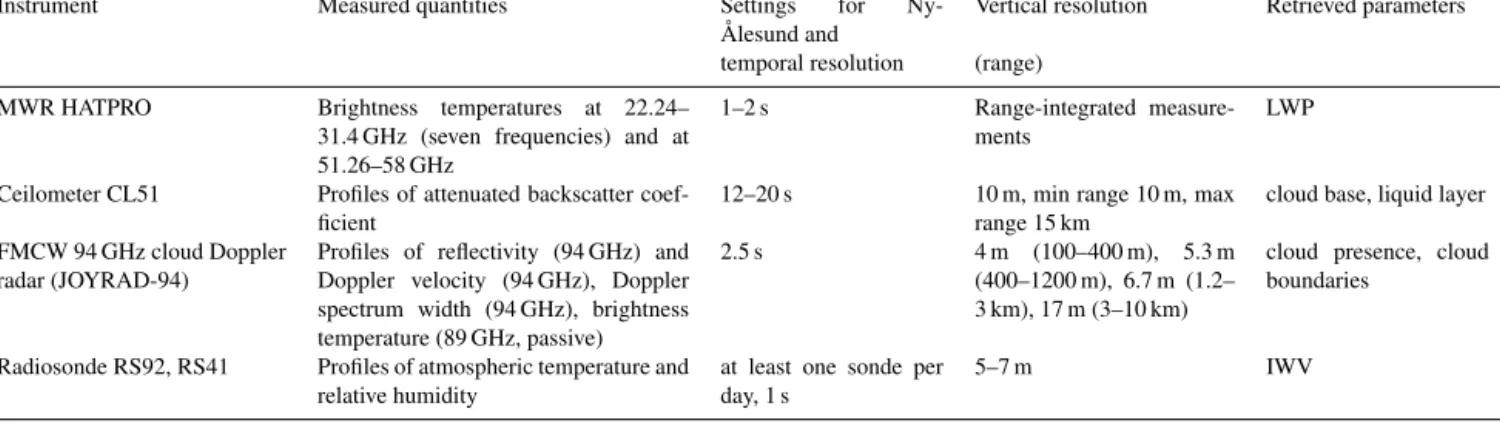
Table 1.Instruments and data used for this study.

Instrument Measured quantities Settings for Ny-

Ålesund and

Vertical resolution Retrieved parameters temporal resolution (range)

MWR HATPRO Brightness temperatures at 22.24–

31.4 GHz (seven frequencies) and at 51.26–58 GHz

1–2 s Range-integrated measure-

ments

LWP

Ceilometer CL51 Profiles of attenuated backscatter coefficient

12–20 s 10 m, min range 10 m, max range 15 km

cloud base, liquid layer FMCW 94 GHz cloud Doppler

radar (JOYRAD-94)

Profiles of reflectivity (94 GHz) and Doppler velocity (94 GHz), Doppler spectrum width (94 GHz), brightness temperature (89 GHz, passive)

2.5 s 4 m (100–400 m), 5.3 m

(400–1200 m), 6.7 m (1.2–

3 km), 17 m (3–10 km)

cloud presence, cloud boundaries

Radiosonde RS92, RS41 Profiles of atmospheric temperature and relative humidity

at least one sonde per day, 1 s

5–7 m IWV

Table 2.Cloudnet characteristics for Ny-Ålesund.

Property Value

Input parameters (instrument and/or model)

LWP (MWR), reflectivity factor and Doppler velocity (94 GHz radar), attenuated backscatter coefficient (ceilometer CL51), hourly model analysis and forecasts (GDAS1 or NWP ICON model)

Temporal resolution 30 s

Vertical resolution (range) 20 m

Retrieved parameters Target classification, IWC

In this study the vertical structure of clouds at Ny-Ålesund is characterized for the first time using lidar–radar synergy. In particular, we used the cloud radar to get information about the cloud structure through the whole atmospheric column.

Instrumentation, data products, and models used in this study are presented in Sect. 2. Thermodynamic conditions at Ny- Ålesund for the investigated time period are shown in Sect. 3.

In Sect. 4 the vertical hydrometeor distribution and occurrence of different cloud types at Ny-Ålesund are analyzed.

For single-layer clouds, which can be liquid, ice, and mixed phase, liquid and ice water path (LWP and IWP) are derived and discussed. The cloud occurrence is related to thermodynamic conditions such as temperature and humidity (Sect. 4).

Since environment temperature and humidity are some of the main parameters affecting cloud formation and development characterization in models, in Sect. 5 we compare the observed relations between cloud occurrence and thermodynamic conditions with those produced by the numerical weather prediction (NWP) model ICON (Icosahedral Non- hydrostatic; Zängl et al., 2015). Finally, the discussion of results and the summary are given in Sect. 6 and the outlook in Sect. 7.

2 Instrumentation and data products

In this study we use various measurements and products continuously running at the AWIPEV observatory. A set of pas-

sive and active remote sensors provides information about the thermodynamic state and cloud and precipitation profiling. In the following subsections, we give an overview of the instruments, data products, and model data, as well as a short description of the measurement principles and retrieval methods. Table 1 summarizes the measured quantities and retrieved parameters of the instruments. Table 2 gives an overview on the Cloudnet products used for the cloud analysis and provides input parameters and model data for the Cloudnet algorithm.

2.1 Radiosonde observations

Radiosondes have been launched at AWIPEV at least once per day at 11:00 UTC for more than 2 decades (Maturilli and Kayser, 2017a). The radiosondes provide vertical profiles of temperature, humidity, wind speed, and wind direction. From 21 May 2006 to 2 May 2017 all radiosondes were of the type Vaisala RS92 and have been processed using the GRUAN version 2 data processing algorithm (Sommer et al., 2012;

Maturilli and Kayser, 2017a). The processing corrects for errors in temperature and humidity, for instance, temperature uncertainties due to the heating effect by solar radiation, and for humidity errors due to a radiation dry bias (Dirksen et al., 2014). Dirksen et al. (2014) reported that after the GRUAN processing the uncertainties of temperature are 0.25^◦C and 0.15^◦C for daytime and nighttime, respectively, and 4 % for relative humidity at altitudes up to 10 km. Since 2 May 2017

(4)

the type of radiosonde has changed to the new radiosonde type Vaisala RS41. The accuracy of the RS41 radiosonde type reported by the manufacturer is 0.1^◦C for temperature and<2 % for humidity.

In the present study we use the radiosonde data to characterize the thermodynamic state at Ny-Ålesund for the period from June 2016 to July 2017. In addition, we compare atmospheric parameters of the analyzed period with a previous 23-year-long homogenized radiosonde dataset (Maturilli and Kayser, 2016, 2017b). To relate cloud properties to the thermodynamic conditions under which they occur, we combined the radiosonde data with measurements from ground- based instruments operated by AWIPEV.

2.2 Microwave radiometer

At AWIPEV, passive microwave observations have been performed with a humidity and temperature profiler (HATPRO;

Rose et al., 2005) since 2011. HATPRO is a 14-channel microwave radiometer that measures atmospheric brightness temperatures (TBs) at K-band (22.24–31.40 GHz) and V- band (51.26–58 GHz) frequencies with a temporal resolution of 1–2 s. The six K-band channels (22.24, 23.04, 23.84, 22.44, 26.24, 27.84 GHz) are located close to the water vapor absorption line at 22 GHz. The 31.4 GHz channel is located in the atmospheric window. The TBs measured at K-band are used for integrated water vapor (IWV), LWP, and humidity profile retrievals. The seven V-band channels (from 51.26 to 58 GHz) are located along the oxygen absorption complex at 60 GHz and are used for vertical temperature profiling.

A multivariable linear regression algorithm (Löhnert and Crewell, 2003) was applied to the TB observations to derive LWP and IWV as well as temperature and humidity profiles.

In order to determine the site-specific regression coefficients a dataset of almost 3800 Ny-Ålesund radiosondes was used in combination with a radiative transfer model (RTM) to simulate the HATPRO TBs. In addition to GRUAN processing all the radiosonde data were quality controlled according to Nörenberg (2008). To this end, radiosondes that did not reach the 30 km height were extended with climatological profiles.

In order to determine and correct for potential TB offsets, we followed the method by Löhnert and Maier (2012).

The assessment of the TB offsets allows for the reduction of systematic errors in TBs originating from instrumental effects as well as from radiative transfer simulations. For this method, only clear-sky cases were used. In order to identify clear-sky situations, i.e., cases without any liquid, HATPRO zenith measurements were checked within 20 min before and after a radiosonde launch. In particular, we checked standard deviations of the retrieved LWP every 2 min. If all the standard deviation values of the LWP within 40 min did not exceed 1.2 g m⁻², these cases were considered as clear sky.

The TBs measured by HATPRO were then compared to the TBs simulated from the radiosonde data, and mean TB offsets were determined. In this way, a TB offset correction was

performed for each period between two absolute calibrations of the instrument.

For this study, we used the retrieved LWP from HATPRO to get information about the amount of liquid in the atmospheric column. This LWP information is also used in the Cloudnet product, which is presented in Sect. 2.5. The typical uncertainty for the LWP retrieved from HATPRO measurements is 20–25 g m⁻²(Rose et al., 2005). HATPRO measures continuously during the whole day but cannot provide reliable information during rain conditions when the radome of the instrument is wet. In these cases, data have been flagged and excluded from the analysis.

2.3 Ceilometer

Since 2011 a Vaisala ceilometer CL51 has been operated at the AWIPEV observatory (Maturilli and Ebell, 2018). The ceilometer emits pulses at 905 nm wavelength and measures atmospheric backscatter with a temporal resolution of about 10 s and a vertical resolution of 10 m. The maximum profiling range is 15 km.

The ceilometer is sensitive to the surface area of the scat- terers and is thus strongly affected by high concentrations of particles like cloud droplets and aerosols (O’Connor et al., 2005). On the one hand, it is thus well suited to detect liquid layers and cloud-base heights. On the other hand, the near- infrared signal is significantly attenuated by liquid layers.

Therefore, the ceilometer often cannot detect cloud particles above the lowest liquid layer when optical depth exceed a value of around 3.

Protat et al. (2006) reported that ceilometers are essential for the reliable detection of high-level ice clouds. How- ever, a lidar system alone is not sensitive enough to detect clouds with low ice water content of the order of less than 10⁻⁶g m⁻³(Bühl et al., 2013). In this study, the attenuated backscatter profiles of the ceilometer CL51 are used in the Cloudnet product (see Sect. 2.5). The ceilometer is calibrated using the technique by O’Connor et al. (2004), which has uncertainties of 10 %.

2.4 94 GHz radar

On 10 June 2016 a new 94 GHz cloud radar (JOYRAD- 94) of the University of Cologne was installed at AWIPEV station. JOYRAD-94 is a frequency-modulated continuous- wave (FMCW) Doppler W-band radar. The active part of the radar measures at 94 GHz. The radar also has a passive channel at 89 GHz that is well suited for LWP retrievals. Küch- ler et al. (2017) showed the details of the operational principle and signal processing for JOYRAD-94. At Ny-Ålesund JOYRAD-94 is operated in a high-vertical-resolution mode (Küchler et al., 2017). The temporal resolution of the cloud radar is 2.5 s, and the vertical resolution changes with height from 4 to 17 m. Minimum detection height was 100 m above the ground. Table 1 shows the main settings and parameters

(5)

for the high-vertical-resolution mode. JOYRAD-94 data are available from 10 June 2016 to 26 July 2017, when it was re- placed by a similar instrument MIRAC-A. In this study, we restrict the analysis to the first year of measurements when JOYRAD-94 was operating. Profiles of the radar reflectivity factor and the mean Doppler velocity were used in the Cloudnet algorithm to provide information on cloud boundaries, cloud phase, and microphysics.

The Cloudnet algorithm corrects the radar reflectivity for attenuation by atmospheric gases and liquid water. Temper- ature, humidity, and pressure profiles from a model are used by Cloudnet for the corrections. The two-way uncertainty of the gas attenuation estimated by Hogan and O’Connor (2004) is about 10 %. The uncertainty of 25 g m⁻² in LWP from MWR causes about±0.2 dB uncertainty in the two-way attenuation at the W-band (Matrosov, 2009).

The total radar reflectivity uncertainty consists of the cali- bration bias, which is within±0.5 dB (Küchler et al., 2017), the random error, and the gas–liquid attenuation uncertainty.

The random error depends on a number of independent measurements, which for the 30 s Cloudnet sampling varies from 72 to 108 for the radar settings used (see Table 1).

Taking into account the noncoherent averaging of the independent measurements (Bringi and Chandrasekar, 2001, Eq. 5.193) the standard deviation of the random error is of the order of 0.5 dB.

2.5 Cloudnet products

The Cloudnet algorithm suite (Illingworth et al., 2007) com- bines observations from a synergy of ground-based instruments. Cloudnet output includes several products such as a cloud target classification and products with microphysical properties (e.g., ice water content – IWC, liquid water content). In order to provide the full vertical information on clouds, Cloudnet requires measurements from a Doppler cloud radar, a ceilometer–lidar, a microwave radiometer, and thermodynamic profiles of a NWP model. For Ny-Ålesund, measurements are taken from the 94 GHz FMCW cloud radar JOYRAD-94, the ceilometer CL51, and the HATPRO MWR.

Model data are taken from GDAS1 (Global Data Assimila- tion System) or NWP ICON, which will be presented in the next subsection. For the first time, data from a FMCW cloud radar with a varying vertical resolution were implemented in the Cloudnet algorithm. Within Cloudnet, the measurements are scaled to a common temporal and vertical grid of 30 s and 20 m, respectively.

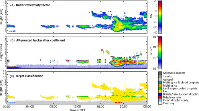
For the target classification the lidar backscatter and Doppler radar parameters are analyzed in combination with thermodynamic profiles of a model (Hogan and O’Connor, 2004). As an example, measurements from the radar and the ceilometer and the Cloudnet target classification on 29 September 2016 are shown in Fig. 3. The target classification consists of the categories (1) aerosols and insects, (2) insects, (3) aerosols, (4) melting ice and cloud

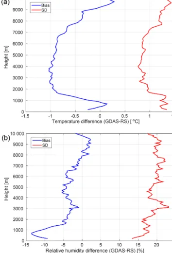
Figure 1. Difference in temperature (a) and relative humidity(b)between GDAS1 and radiosonde data. Radiosondes for the period from February 2017 to July 2017 at Ny-Ålesund are used.

Blue and red lines show the bias and the standard deviation, respectively.

droplets, (5) melting ice, (6) ice and supercooled droplets, (7) ice, (8) drizzle–rain and cloud droplets, (9) drizzle or rain, (10) cloud droplets only, and (11) clear sky. In this study, the Cloudnet target categorization is used to differentiate cloud phase (liquid, ice, and mixed phase) and to identify different cloud types.

For the classification the Cloudnet algorithm identifies the 0^◦C isotherm using the wet-bulb temperature calculated from the model data. Therefore, the model uncertainties (Figs. 1 and 2) may lead to liquid–ice misclassification at temperatures close to 0^◦C. In the case of precipitating clouds uncertainties of the model are mitigated by the Cloud- net algorithm using radar Doppler observations. The algorithm identifies the 0^◦C isotherm by a significant gradient in the particle vertical velocity.

Based on the target classification, various cloud microphysical retrievals are applied within Cloudnet. The Cloud- net IWC product, which is used in this study, is based on a

(6)

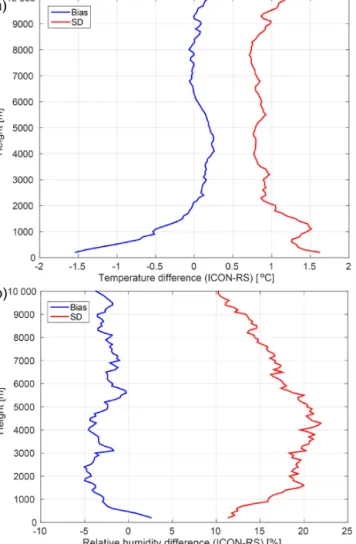
Figure 2.Difference in temperature(a)and relative humidity(b) between the ICON column output over Ny-Ålesund and radiosonde data for the period from February 2017 to July 2017. Blue and red lines show the bias and the standard deviation, respectively.

Z–IWC–T relation (Hogan et al., 2006; Heymsfield et al., 2008) where Z is a radar reflectivity factor and T the air temperature. The Cloudnet IWC has a bias error and typical random error of 0.923 and 1.76 dB, respectively. Hogan et al. (2006) found that uncertainties of the IWC retrieval dif- fer for different temperature ranges and are estimated to be from−50 % to+100 % for temperatures below−40^◦C and ranging from−33 % to 50 % for temperatures above−20^◦C.

The numbers here are root mean squared errors given with respect to the reference IWC. Evaluating the method of Hogan et al. (2006); Heymsfield et al. (2008) resulted in similar uncertainties, except that there was a positive bias of about 50 % for temperatures above−30^◦C. The authors estimated the uncertainties from 0 % to +100 % and from −50 % to +100 % at temperatures above and below −30^◦C, respectively. The uncertainty in the radar reflectivity also influences the IWC retrieval. The total uncertainty of 2 dB corresponds to a range of about+40 % to−30 % uncertainty in IWC. Part

of this uncertainty is to be included into the uncertainty of the Z–IWC–T relation from Hogan et al. (2006) because the relation was found empirically using radar observations. More detailed information on the Cloudnet products can be found in Illingworth et al. (2007).

For the analyzed period (June 2016–July 2017), the Cloud- net availability is more than 90 % for most of the months (Fig. 4). Exceptions are June 2016 (installation of the radar on 10 June), July 2016, and February 2017 (new software installation for cloud radar) with a data coverage of 64 %, 85 %, and 81 %, respectively. The total number of analyzed Cloud- net profiles is 1 130 030, which includes 216 860 clear-sky profiles and 913 170 cloudy profiles.

2.6 Model data

2.6.1 Global data assimilation system GDAS1

The Global Data Assimilation System (GDAS; Kanamitsu, 1989) is operated by the US National Weather Service’s Na- tional Centers for Environmental Prediction (NCEP). This system analyzes different types of observations and maps the results on a grid used for model initializations. The GDAS dataset is initialized every 6 h and outputs an analysis time step followed by forecasts with a temporal resolution of 3 h on 23 pressure levels.

In the present study GDAS1 data (see https://www.ready.

noaa.gov/gdas1.php, last access: 28 February 2019, for detailed information), which are available on a 1^◦ by 1^◦ latitude–longitude grid, were used in the Cloudnet algorithm to provide thermodynamic information for the period from 10 June 2016 to 31 January 2017. The vertical resolution varies from 173 m near the ground to 500 m at a height of 2 km and to∼2.5 km at a height of 15 km. The uncertainties of the temperature and relative humidity profiles of GDAS1 are shown in Fig. 1. The maximum errors in temperature and relative humidity do not exceed−1±1.5^◦C and−15±24 %, respectively.

2.6.2 NWP ICON model

The ICOsahedral Non-hydrostatic (Zängl et al., 2015) modeling framework for global NWP and climate modeling is developed by the German Weather Service and the Max Planck Institute for Meteorology. The grid structure of ICON is based on an icosahedral (triangular) grid with an average resolution of 13 km. The averaged area of the triangular grid cells is 173 km². In the vertical dimension, the model has 90 atmospheric levels up to a maximum height of 75 km. The vertical resolution ranges from 30 m at the lowest heights to about 500 m at about 15 km of height. The vertical resolution at a 2 km height is about 260 m. For this study we used a column output for Ny-Ålesund taken from the operational global ICON model run. In particular, vertical profiles of environment temperature and humidity, specific cloud wa-

(7)

Figure 3.Radar reflectivity factor(a), lidar backscatter coefficient,(b)and Cloudnet target classification(c)on 29 September 2016; AWIPEW observatory at Ny-Ålesund.

Figure 4.Cloudnet data availability for Ny-Ålesund for June 2016 to July 2017. Grey bars correspond to clear-sky profiles, black bars to cloudy profiles, and white space means no Cloudnet data availability.

ter content, specific cloud ice content, rain mixing ratio, and snow mixing ratio were used in this study. The ICON column output for Ny-Ålesund is available since 1 February 2017 and has been used as an input for the Cloudnet algorithm since then.

In this study, we use ICON data to exemplarily show how such an observational dataset of clouds can be used for a

model evaluation (Sect. 5). We relate the occurrence of different types of clouds in the ICON model to temperature and humidity and compare the results to the observational statistics. ICON model output for Ny-Ålesund is available twice a day at 00:00 and 12:00 UTC with a forecast for 7.5 days (180 h) and hourly output intervals. The data only from the first 12 h after the initialization of the model run were used in our analysis. The uncertainties of the temperature and relative humidity profiles of the ICON model are shown in Fig. 2.

The maximum errors in temperature and relative humidity at an altitude up to 10 km are −1.5±1.5^◦C and −5±20 %, respectively.

3 Thermodynamic conditions

It is well known that environmental temperature and humidity strongly influence cloud formation and development.

Therefore, we start our analysis with an insight into the thermodynamic conditions during the study period. In this section we also check how representative this time period is in terms of thermodynamic conditions in comparison to the long-term mean.

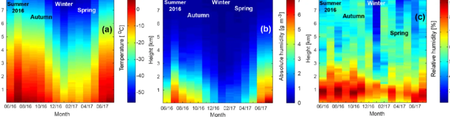
Figure 5a shows the monthly mean atmospheric temperature based on the radiosonde data for the period from June 2016 to July 2017. The atmospheric temperature fol- lows an annual cycle typical for the Northern Hemisphere with higher temperatures during summer and autumn and lower temperatures in winter and spring. The lowest values

(8)

Figure 5.Vertical profiles of monthly mean atmospheric temperature(a)and absolute(b)and relative humidity(c)from radiosonde observations at Ny-Ålesund from June 2016 to July 2017.

of the monthly mean temperature in the lowest 50 m were observed in March and January 2017 (−11 and−10^◦C, respectively). The highest observed monthly mean temperature was+7^◦C in July 2016. Looking at the monthly mean temperature at 5 km of height, minimum and maximum values of−41 and−17^◦C were found in January and July, respectively. Despite the fact that Ny-Ålesund is located at the coastline where the climate is supposed to be less variable due to the impact of the ocean, the monthly mean temperature changes by 19 and 24^◦C in the lowest 50 m and 5 km of height, respectively. This large amplitude of the temperature change at Ny-Ålesund can be explained by the regular occurrence of polar day and polar night. When a polar night begins in the beginning of October, atmospheric temperature dramatically decreases and it starts to increase again in late March (Fig. 5a). Moreover, the smaller temperature variance at lower altitudes might be related to processes between the surface and the atmosphere and the conserved energy near the ground.

Figure 5b provides information on monthly mean absolute humidity from June 2016 to July 2017. In summer the water vapor is mostly concentrated in the lowest 1.5 km with the highest monthly mean values of up to 6 g m⁻³in July 2016 and July 2017. The water vapor in this altitude range is thus the main contributor to the integrated water vapor (IWV). In winter, the monthly mean absolute humidity is much lower with a minimum value of∼1.5 g m⁻³(January) in the lowest 1.5 km.

In terms of relative humidity with respect to water (RH_w, Fig. 5c), it can be seen that the monthly mean RH_wis highest in the lowest 2 km of the atmosphere. This is in agreement with Maturilli and Kayser (2017a). There is no strong seasonal variability of the monthly mean RH_wat altitudes higher than 4 km. In the lower troposphere, the monthly mean RH_w, following the temperature cycle, is higher in summer and autumn (ranging from 60 % to 94 % in the lowest 2 km) and lower in winter and spring (ranging from 52 % to 81 % in the lowest 2 km), except for March 2017. In March 2017, the coldest month in the period of this study, the monthly

mean absolute humidity was relatively low (1.7 g m⁻³) in the lowest 1.5 km, while monthly mean RH_w was up to 85 % (Fig. 5c). In summer and autumn months high values of monthly mean RH_woccur from the surface to 1.7 km. In winter and spring, the atmospheric layer near the surface is drier and high values of RHwappear from 0.3 to 1.5 km.

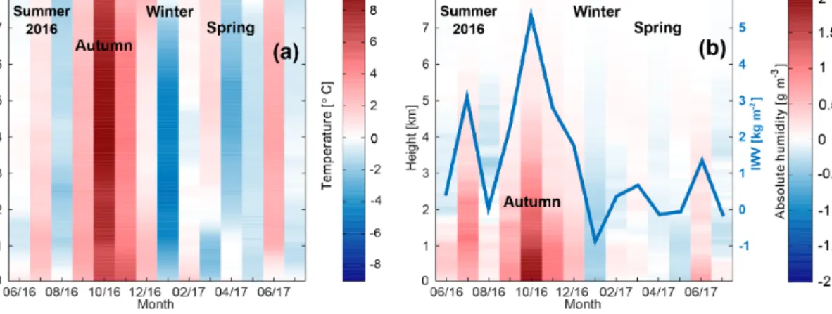
In order to determine if and in which way the thermodynamic properties were special for the study period, monthly mean tropospheric temperature anomalies are presented in Fig. 6a. These anomalies have been calculated with respect to the previous 23 years (1993–2015). Figure 6a shows that, compared to the long-term mean, temperatures are higher for some particular summer months. For example, July 2016 and June 2017 were warmer throughout the whole troposphere with maximum temperature anomalies of up to 2 and 4^◦C, respectively. Winter months were slightly warmer, too: the difference in atmospheric temperature was up to 2^◦C in De- cember 2016 and February 2017. January 2017 was much colder with a temperature difference of down to−5^◦C. In comparison to the previous 23 years, atmospheric temperatures in March 2017 were higher in the upper troposphere (up to 2^◦C) and lower (−2^◦C) in the lowest 1.5 km. The largest positive temperature difference was found for autumn 2016, especially for October 2016 with maximum temperature differences of up to+8^◦C. Johansson et al. (2017) have already shown that moisture intrusions from the North Atlantic can cause significant local warming in some regions of the Arc- tic that can reach up to 8^◦C. In addition, Overland et al.

(2017) analyzed the variability of the near-surface air temperature (at 925 mb level) in the Arctic for the period from October 2016 to September 2017. The authors reported that there was an extreme temperature anomaly exceeding 5^◦C in the autumn 2016 that is in agreement with our results. More- over, the authors showed that this extremely high temperature anomaly was associated with a persistent and unusual pat- tern in the geopotential height field that separated the polar vortex in the central Arctic into two parts. This situation led to southerly winds that transported warm air into the Arctic

(9)

from the midlatitude Pacific and Atlantic oceans (Overland et al., 2017).

The observed anomalies in the monthly mean absolute humidity and IWV (Fig. 6b) in principle follow the sign of the discussed temperature anomalies. Figure 6b shows a correlation between the temperature and IWV increase. For instance, months that have a positive temperature difference also have an increase in the absolute humidity and IWV. Neg- ative temperature differences correspond to decreases in the absolute humidity. For example, January 2017 was particularly colder and drier with anomalies in absolute humidity and IWV of∼ −0.5 g m⁻³and∼ −0.8 kg m⁻², respectively.

Higher IWV values in comparison with the previous years were observed in June 2016, autumn 2016, December 2016, and July 2017. The differences in IWV varied from 1 to 5 kg m⁻²with the largest contributions from the lowest 3 km.

In October 2016, the absolute humidity anomaly was highest (∼2 g m⁻³) in the lowest 3 km. This led to a positive change in IWV of more than 5 kg m⁻²in comparison with previous years.

Thus, it turns out that the period of our study had specific features especially for some months. Maturilli and Kayser (2017a) have shown that in general a significant warming of the atmospheric column at Ny-Ålesund is observed in Jan- uary and February. The authors reported that this warming in winter is related to the higher frequency of large-scale flow from south-southeast and less from the north. However, in our study January 2017 was much colder in comparison to the previous years. In January 2017, and also in the other winter months, the wind direction occurred more frequently from south-southwest (not shown) in comparison with the earlier period from 1993 to 2014 with wind direction domi- nating from the southeast. However, it is not clear yet what exactly caused the relatively cold January 2017.

4 Results

4.1 Hydrometeor occurrence

From June 2016 to July 2017, cloudy profiles occur around 80 % of the time (Fig. 7). The frequency of cloud occurrence is largest in October 2016 and June 2016 (∼92 %) and lowest in April 2017 (68 %). In order to have a closer look at which types of hydrometeors occur in the atmospheric column, Fig. 7 also gives separate overviews of the frequency of occurrence of liquid and ice hydrometeors.

For this statistics we check all the range bins in Cloudnet profiles for hydrometeor types. If a Cloudnet bin contains cloud droplets, rain, or drizzle we count it as liquid. If ice particles have been detected in a range bin, then we define it as ice. Note that Cloudnet does not distinguish between snow and cloud ice. Mixed-phase range bins are considered as both liquid and ice. Then profiles that contain at least one

“liquid” (“ice”) bin are counted as liquid (ice) containing.

Profiles containing liquid and ice phases are counted in both classes.

Liquid hydrometeors (dashed black line in Fig. 7) have the highest frequency of occurrence during summer and autumn (70 %–80 %) and the lowest in winter (∼36 %). A pronounced seasonal variability is thus visible. Ice (densely dashed black line in Fig. 7) occurs more often in autumn, winter, and early spring with the frequency of occurrence varying from 72 % to 88 %. In summer ice occurs typically around 58 %–78 % of the time. The frequency of ice occurrence does not show a clear seasonal variability like the liquid phase.

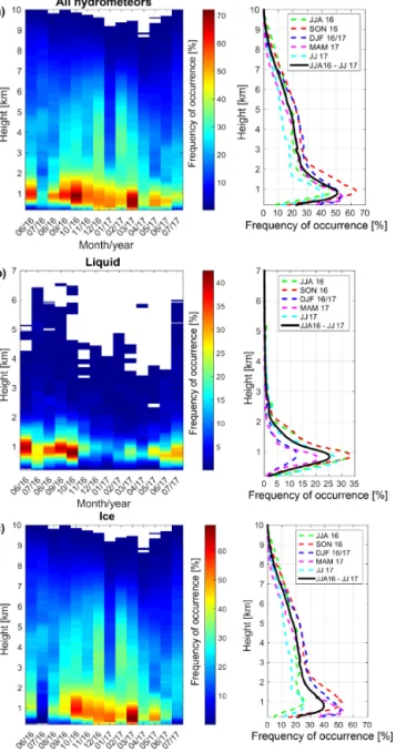
Figure 8 shows vertical distributions of hydrometeors. For these statistics we used the abovementioned bin classification. The frequency of occurrence at a certain altitude was normalized to the total number of Cloudnet profiles in a cor- responding month. The highest frequency of occurrence was 60 % and 70 % in March 2017 and October 2016, respectively (Fig. 8a, left). The lowest frequency of occurrence was in July 2016 (<30 %), while for the other months in summer 2016 the frequency of occurrence of all hydrometeors was around 60 %. In January 2017 the occurrence of clouds above 3 km was less than 10 %, which correlates with low RH_w(Fig. 5c) at these altitudes and the lowest value of IWV (Fig. 6b).

The total vertical distribution (Fig. 8, right panels, solid black line) shows that hydrometeors occur predominantly in the lowest 2 km with a maximum frequency of occurrence of∼53 % at a height of 660 m. Above 2 km, the frequency of occurrence is less than 30 % and monotonically decreases with height. In terms of seasons, the vertical frequency of occurrence of all hydrometeors reveals variations in the maximum within±10 % with the highest values of frequency of occurrence in autumn 2016 of more than 60 % (∼1 km of height). In summer 2016, the hydrometeor frequency of occurrence is in general higher than in summer 2017, indicating a pronounced year-to-year variability that will be analyzed in the future when multiyear datasets become available.

Liquid hydrometeors (Fig. 8b) occur most of the time in the lowest 2 km. Above 2 km, the frequency of occurrence of liquid is less than 5 % and above 3 km almost no liquid particles are observed. The frequency of occurrence of liquid has a maximum at around 0.7–0.9 km of height. Largest values of liquid-phase occurrence vary from 40 % to 50 % in summer and autumn 2016. The maximum frequency of occurrence in the winter months does not exceed 15 %. A strong seasonal variability of liquid, with high values in summer (32 %) and lowest values in winter (12 %), can be seen.

The vertical occurrence of ice hydrometeors is shown in Fig. 8c. Ice is mostly present at altitudes below 2 km. On average the frequency of occurrence peaks at around 700 m with values of 40 %. In contrast to the ice occurrence any- where in a column (Fig. 7), which does not show a strong seasonal variability, the vertical distribution of the ice phase shows a pronounced seasonal cycle, in particular in the low-

(10)

Figure 6.Anomalies of monthly mean atmospheric temperature(a)and absolute humidity(b)from radiosonde observations at Ny-Ålesund from June 2016 to July 2017. Anomalies are calculated with respect to the monthly mean values of the previous 23 years (1993–2015). The blue line corresponds to the IWV anomaly for the same time period.

Figure 7.Frequency of occurrence of profiles with ice, liquid, and any kind of hydrometeor. The frequency is given in % and normalized to the total number of Cloudnet profiles for each month.

est 2 km. For higher altitudes, the seasonal variability is less pronounced. Above 2 km, the frequency of occurrence of ice decreases from∼30 % to less than 10 % at 8 km.

Similar to liquid hydrometeors, the frequency of occurrence of ice is highest in the lowest 2 km with values of 60 % and 70 % in October 2016 and March 2017, respectively (Fig. 8c, left). The lowest ice frequency of occurrence is found for the summer months. In July 2016, which is the warmest month during the observation period, the freezing level often reached altitudes up to 2 km and therefore almost no ice was observed below this height. In January 2017 ice rarely occurred at heights above 4 km, which was probably caused by the presence of dry air. On the right side of Fig. 8c it can be seen that the highest frequency of occurrence of the ice phase is in the lowest 2 km and around 52 % in autumn, winter, and spring.

4.2 Statistics on different types of clouds

In addition to the occurrence of hydrometeor types, a classification of clouds into single-layer and multilayer was also made. Single-layer clouds were furthermore separated into liquid, ice, and mixed phase.

For the classification every Cloudnet profile was checked from the top to the bottom for cloud layers. A cloud is defined here as a layer of at least three consecutive cloudy height bins. Based on a number of identified cloud layers we classified single-layer and multilayer clouds. We considered cases as multilayer if two or more cloud layers were separated by one or more clear-sky height bins. Figure 9 gives an overview of the cloud type occurrence at Ny-Ålesund for the whole period of this study. The total occurrence for the whole period (rightmost bar) shows 44.8 % (506 253 profiles) multilayer and 36 % (406 810 profiles) single-layer clouds.

Among single-layer clouds the most frequent type was mixed phase, followed by ice and liquid single-layer clouds with cloud occurrence of 20.6 %, 9.0 %, and 6.4 %, respectively.

Note that clouds were considered mixed phase if ice and liquid phases were both present in the same cloud boundaries regardless of whether liquid and ice were in the same range bin or not. This implies that mixed-phase clouds in- clude not only cases with liquid cloud top and ice below, but also cases when both phases (ice and liquid) are present any- where within the detected cloud layer.

Figure 9 also shows the monthly occurrence of different cloud types. The monthly cloud occurrence, i.e., the sum of all different cloud types, corresponds to the frequency of occurrence of all hydrometeors shown by a solid black line in Fig. 7. As seen for liquid and ice hydrometeors (Fig. 7), the occurrence of single-layer liquid and ice clouds also has a seasonal and monthly variability. About 15 % of single-layer liquid clouds were detected in summer but less than 2 % in other seasons. The occurrence of single-layer ice clouds was 15 %–20 % in winter and spring and less than 5 % in

(11)

Figure 8.Monthly, seasonal, and total (for the whole time period) frequency of occurrence of all hydrometeors (a), liquid (b), and ice(c)as a function of height for the period from June 2016 to Au- gust 2017. Frequency of occurrence is given in % and normalized to the total number of Cloudnet profiles for each month.

other months. Single-layer mixed-phase clouds and multilayer clouds were present most of the time with typical values of frequency of occurrence of around 20 % and 45 %, respectively. Thus, most of the time cloud systems had a complicated structure and/or consisted of both phases, liquid and ice, indicating that they are related to complex microphysical processes. In turn, the observational capabilities of these types of clouds are limited. In situations with multiple liquid layers, whether warm or mixed phase, partitioning the observed LWP from HATPRO among these different layers

Figure 9. Monthly frequency of occurrence of different types of single-layer clouds (liquid, ice, and mixed phase), multilayer clouds, and clear-sky profiles for the period from June 2016 to July 2017. The last right column shows the total frequency of occurrence.

is particularly challenging and results in larger uncertainties (Shupe et al., 2015). A multilayer cloud classification requires a reliable profiling of liquid layers, which is limited by significant attenuation of lidar signals in the first liquid layer.

Radar signals have better propagation through the whole vertical cloud structure in comparison with a lidar. However, the radar reflectivity is often dominated by scattering from relatively large particles, which masks the presence of small particles, like liquid droplets, present in the same volume. In the case of multilayer mixed-phase clouds, the liquid phase thus cannot be reliably detected based on radar reflectivity alone.

4.3 Single-layer clouds and their relation to thermodynamic conditions

Taking into account the abovementioned limitations of multilayer cloud observations, our further analysis is concentrated only on single-layer cases. For the following analysis of single-layer clouds we also used LWP from HAT- PRO and the Cloudnet IWC product. We excluded cases for which this information was not available. In particular, profiles with the presence of liquid precipitation and flagged data due to wet HATPRO radome were excluded. The result- ing dataset (Fig. 10, lines with circles, stars, and diamonds) was thus reduced to 149 960 profiles (37 % of all single- layer profiles) with 65 299 profiles (16 %) for single-layer mixed-phase clouds, 59 364 profiles (15 %) for single-layer ice clouds, and 25 297 profiles (6 %) for single-layer liquid clouds only. Thus, all results are relevant for single-layer clouds without liquid precipitation. Nevertheless, with this subset of single-layer clouds we can still capture the monthly variability and thus assume that it is still representative for all single-layer cloud cases.

(12)

Figure 10.Frequency of occurrence of ice-only, liquid-only, and mixed-phase single-layer clouds based on Cloudnet categorization data (for lines with circles, diamond and star profiles with liquid precipitation are not included). The frequency is given in % and normalized to the total number of Cloudnet profiles in each month.

A comparison of Figs. 10 and 9 shows that the occurrence variability of liquid and ice single-layer clouds is similar. The occurrence of mixed-phase clouds differs because of the exclusion of liquid precipitation clouds, which often contain an ice-phase and melting layer, and are thus considered mixed phase. This is in agreement with Mülmenstädt et al.

(2015), who reported that most liquid precipitation is formed including the ice phase. The maximum and minimum occurrences of single-layer mixed-phase clouds (25 % and 4 %) were observed in May 2017 and June 2016, respectively.

The annual-averaged top height of single-layer mixed-phase clouds was 2 km (not shown). Our findings are in good agreement with spaceborne radar–lidar observations of clouds in the Svalbard region in the period from 2007 to 2010 (Mioche et al., 2015). It has been shown that single-layer mixed-phase clouds in the Svalbard region mostly occur in May.

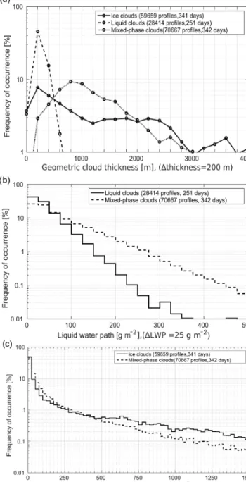
The geometrical thickness of single-layer clouds is shown in Fig. 11a. The geometrical thickness of a cloud is calculated as the distance between the upper border of the up- permost cloud range bin and the lower border of the low- ermost cloud range bin. The thickness of single-layer liquid clouds varies between 60 and 2200 m with mean and median values of 280 and 240 m, respectively. Less than 1 % of observed single-layer liquid clouds have a thickness larger than 800 m. In contrast, single-layer mixed-phase clouds typically have a larger geometrical cloud thickness, which varies from 100 to 8500 m with median and mean values of 1100 and 1500 m, respectively. In comparison with mixed- phase single-layer clouds, the geometrical cloud thickness distribution for single-layer ice clouds is broader, ranging from 60 to 9500 m. The median and mean values of the geometrical cloud thickness for single-layer ice clouds are 1500 and 2100 m, respectively. The mode of the thickness distribution of single-layer ice clouds corresponds to 800 m.

Less than 1 % of single-layer mixed-phase and ice clouds

Figure 11.Frequency of occurrence of cloud thickness for single- layer clouds (a), LWP for single-layer liquid and mixed-phase clouds(b), and IWP for single-layer ice and mixed-phase clouds(c) for the period from June 2016 to July 2017. Theyaxis is shown in logarithmic scale. In thexaxes1shows the bin width. The frequency of occurrence is normalized by the total number of corre- sponding cloud types.

have a geometrical cloud thickness larger than 3 and 4.2 km, respectively.

The frequency of LWP occurrence for liquid and mixed- phase clouds is shown in Fig. 11b. Both types of clouds are characterized by relatively low values of LWP. The median values of LWP for single-layer liquid and mixed-phase clouds are 17 and 37 g m⁻², and mean values are 30 and

(13)

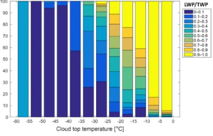
Figure 12.The relative probabilities of different ranges of the liquid fraction LWP/TWP given at various cloud-top temperatures of single-layer mixed-phase clouds. The probability is normalized by the total number of profiles for each cloud-top temperature range.

Numbers at the top of plot show the number of cases included in the temperature range. The total number of profiles is 3824.

66 g m⁻², respectively. More than 90 % of single-layer liquid and mixed-phase clouds have LWP values lower than 100 and 200 g m⁻², respectively. It has to be noted that particularly in these LWP ranges, the relative uncertainty in the retrieved LWP is quite large (see Sects. 2 and 2.2). Larger LWP values in mixed-phase clouds might be related to their larger geometrical thickness (Fig. 11a).

Median values of IWP for single-layer ice and mixed- phase clouds are 14.6 and 21.4 g m⁻², and mean values are 273 and 164 g m⁻², respectively (Fig. 11c). IWP values exceeding 400 g m⁻² are more frequent in single-layer ice clouds than in single-layer mixed-phase clouds. However, for both cloud types the occurrence of IWP values higher than 125 g m⁻²is less than 3 %.

A number of studies comparing observed and modeled LWP and IWP values for Arctic regions have revealed the challenge for NWP models to accurately simulate LWP and IWP. Tjernström et al. (2008) evaluated six regional models that were set to a common domain over the western Arc- tic and found that one-half of the models showed nearly 0 bias in LWP, while the other half underestimated LWP by

∼20 g m⁻². The authors reported that some of the models showed −30 to 30 g m⁻² biases in IWP. In addition, a low correlation between the observations and modeled IWP and LWP was found. Most of the models showed too-low variability of IWP. Karlsson and Svensson (2011) compared nine global climate models in the Arctic region. The authors showed that means and standard deviations of modeled IWP and LWP can vary by a factor of 2. Forbes and Ahlgrimm (2014) concluded that such discrepancies may be related to an insufficient representation of microphysical processes. The authors note that some of the major challenges are phase partitioning and a parameterization of cloud particle formation and development.

Klein et al. (2009) compared 26 models with airborne and ground-based observations over north Alaska (Barrow and Oliktok Point). The authors found that although many models showed an LWP exceeding IWP (as observed), simulated LWP values were significantly underestimated. Since climate and NWP models typically parameterize cloud phase as a function of temperature, we thus analyzed relations between temperature and phase partitioning for mixed-phase clouds at Ny-Ålesund. Figure 12 shows the probability of liquid fraction, i.e., (LWP/(LWP+IWP)), in mixed-phase clouds for different cloud-top temperature ranges based on the Ny-Ålesund radiosonde observations. In general, the liquid fraction increases with cloud-top temperature. Thus, high liquid fraction values in single-layer mixed-phase clouds are found at cloud-top temperatures ranging from−15 to 0^◦C.

The occurrence of the liquid fraction of 0.4–0.6, implying that both phases are roughly equally present, is relatively high for cloud temperature ranges between−25 and−15^◦C but is rare for cloud-top temperatures below −25^◦C. Al- most no liquid was observed at cloud-top temperatures below

−40^◦C. A nonzero liquid fraction below−40^◦C is mostly associated with thick clouds having high cloud tops with liquid layers detected at lower altitudes.

In-cloud atmospheric temperature and humidity are important for NWP models as these parameters determine cloud particle formation and development. For instance, laboratory studies show that the shapes of ice crystals are defined by the environment temperature and humidity (Fukuta and Taka- hashi, 1999; Bailey and Hallett, 2009). There is also some evidence that similar effects happen in the real atmosphere (Hogan et al., 2002, 2003; Myagkov et al., 2016). Aggrega- tion efficiency and deposition growth rate are also temperature and humidity dependent (Hosler and Hallgren, 1960;

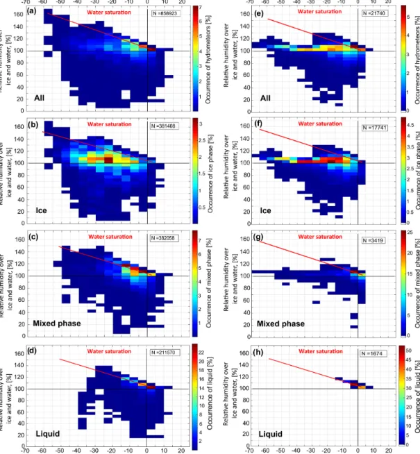
Bailey and Hallett, 2004; Connolly et al., 2012). Therefore, in this study we also relate different cloud types to the environmental conditions under which they occur. The frequency of occurrence of the different hydrometeors in single-layer clouds as a function of in-cloud temperature and relative humidity observed at Ny-Ålesund is shown in Fig. 13a–d. Here, temperature and relative humidity were determined for each cloud bin between cloud boundaries. For this analysis we only used single-layer cloud profiles observed 1 h before and after a radiosonde launch. We assumed that the atmospheric conditions did not change too much within this time period.

For temperatures lower than 0^◦C the relative humidity with respect to ice (RHi) was used. Values of RHwwere used at temperatures exceeding 0^◦C. For the cloud classification we used the method specified in Sect. 4.2.

All single-layer clouds were observed in the temperature range from−60 to+10^◦C (Fig. 13a). In some cases single- layer clouds appeared at low RH_i and RH_w (Fig. 13a–d) that might be associated with hydrometeors falling from saturated to subsaturated atmospheric layers. Another reason could be that the radiosondes, which drift, do not provide representative information for the sampling volume of the

(14)

Figure 13.Two-dimensional histograms of in-cloud atmospheric temperature and relative humidity for all clouds(a, e), ice clouds(b, f), and mixed-phase clouds(c, g). For(a, c, e, g)ice and/or liquid phases are present. For(b)and(f)only the ice phase is present. The liquid phase of liquid-containing clouds is shown in(d)and(h). Only cases of single-layer clouds are included and shown for observations(a–d)and for column output of the NWP model ICON over Ny-Ålesund(e–h). Frequency of occurrence is normalized by the total number of bins of the correspondent single-layer clouds detected between the period of 1 h before and after radiosonde launch.

zenith-pointing ground-based instruments. However, cases with very low relative humidity values occurred in less than 1 % of the analyzed observations. According to McGrath et al. (2006) the uncertainties in temperature due to radiosonde drifts in the Northern Hemisphere do not exceed 0.4^◦C up to 10 km of altitude. Uncertainties in relative humidity are about 3 %.

Figure 13b shows that ice clouds mostly occur in the temperature range from−45 to−5^◦C, including the temperature range (<−38^◦C) of homogeneous nucleation. The highest

occurrence of ice was observed in the temperature range from−25 to−20^◦C and under conditions that are subsaturated with respect to water but saturated with respect to ice (Fig. 13b). Observed ice particles mostly occur at RHis between 100 % and 125 %. The presence of ice at positive temperatures might be related to cases of cloud type misclassification, for example when a cloud was identified as ice in- stead of mixed phase. These cases might also be associated with uncertainties in the model temperature profile used in the classification algorithm.

(15)

Mixed-phase clouds were observed at supersaturation with respect to ice (Fig. 13c). Most of the cases were located at the water saturation line. Frequently, the mixed phase occurs at temperatures from −25 to +5^◦C with two maxima in the range of−15 to 0^◦C. The temperatures−15 and−5^◦C correspond to the highest efficiency of the deposition growth of ice crystals at water saturation levels (Fukuta and Takahashi, 1999).

The liquid phase mostly occurs near water saturation at temperatures from−15 to+5^◦C (Fig. 13d). Supercooled liquid was observed at temperatures down to−40^◦C. The lowest temperature limit for liquid clouds only was−30^◦C (not shown).

5 Application for model evaluation

This observational cloud dataset can provide useful information for a model evaluation. As an example, this section presents a comparison of the NWP model ICON with the observations at Ny-Ålesund. Note that the intention here is not to perform a thorough model evaluation but to show the potential of such a dataset to test, for example, if the de- pendence of the occurrence of clouds on the thermodynamic conditions can be represented by the model.

The statistics on different types of clouds, their phases, and the relation to atmospheric conditions provide a useful dataset for comparison with similar statistics based on the model output.

Based on a 10⁻⁷kg kg⁻¹ threshold in specific cloud water content, specific cloud ice content, rain mixing ratio, and snow mixing ratio, we identify clouds in the model. We clas- sify the clouds using the same procedure as for the observations (see Sect. 4.2). The value of the threshold in the hydrometeor contents was found empirically: the usage of a lower threshold leads to the higher occurrence of ice clouds in the ICON model that were not identified in observations.

For a higher threshold fewer ice clouds were present in the ICON model than in observations. According to theZ–IWC–

T relation from Hogan et al. (2006), the chosen threshold in the ice mixing ratio corresponds to the radar reflectivity factor ranging from−55 to−32 dBZ at temperatures from

−60 to−5^◦C. In general, these values are close to the radar sensitivity, although at high altitudes the radar sensitivity is about−40 dBZ (Küchler et al., 2017). Nevertheless, most of the observed hydrometeors are located within 2 km of the surface (see Sect. 4.1), and therefore the lack of sensitivity at high altitudes does not significantly affect the results. For a more detailed analysis of the uncertainties due to differences between the instrument and the model, sensitivity tests can be done using observation simulators (e.g., Haynes et al., 2007).

Such an analysis is out of the scope of the current study.

The right panels in Fig. 13 show the frequency of occurrence of different hydrometeors in single-layer clouds as a function of in-cloud temperature and RH_w based on the

ICON model data. Figure 13e shows that modeled single- layer clouds occur within the temperature range similar to the temperatures observed in clouds at Ny-Ålesund (Fig. 13a).

Figure 13f indicates that ice clouds in the ICON model typically exist at temperatures from −65 to −5^◦C. Both the ICON model and observations reveal that ice particles typically occur at relative humidities higher than the saturation over ice but lower than the saturation over water. High occurrence of the ice phase in ICON is found at RH_iup to 110 %, while the observations reveal RH_iof up to 125 % (Fig. 13b).

The presence of ice particles at lower supersaturation over ice in the ICON model in comparison with observations may be associated with ice nuclei (IN) parameterization in the ICON model, which is known to still be a challenge (Fu and Xue, 2017). We speculate that a higher concentration of IN and thus ice particles leads to faster deposition of water vapor onto the ice particle surface. Therefore, a more efficient vapor-to-ice transition in the model could lead to lower relative humidity. Similarly, the parameterization of deposition growth rate and secondary ice processes may also have an impact on the in-cloud relative humidity.

Mixed-phase clouds in the ICON model appear near the water saturation (Fig. 13g) that is consistent with the observations (Fig. 13c). The model mostly produces mixed-phase clouds within the temperature range from −10 to +5^◦C, which is narrower in comparison to the observations.

Modeled liquid phase occurs near water saturation at temperatures from−15 to+5^◦C (Fig. 13h), which is in good agreement with observations. In the ICON model the occurrence of the liquid phase at temperatures below−5^◦C is only 6 %, while in the observations this occurrence is more than 30 %.

Figure 14 summarizes the temperature dependencies of hydrometeor occurrences in the ICON model and in observations. The temperature distributions of single-layer liquid clouds (solid red lines, Fig. 14) are narrow (−10 to+5^◦C) for both the model and observations, although the observed distribution has larger values of occurrence. The total distributions of the liquid phase (dashed red lines, Fig. 14) are different. The observed distribution is larger and occupies a wider temperature range (−25 to+10^◦C). In the model, most of the liquid phase is concentrated in the temperature range from−10 to+5^◦C. This difference leads to a divergence between mixed-phase cloud occurrences (solid green lines, Fig. 14): the observed frequency distribution for mixed-phase clouds shows a broader temperature range than the model. Sandvik et al. (2007) showed a similar difference between observed and modeled single-layer mixed- phase clouds. For the modeling, the polar version of the non- hydrostatic mesoscale model from the National Center for Atmospheric Research was used. The authors found that for temperatures below−18^◦the liquid fraction in single-layer mixed clouds was completely absent in simulations.

Ice cloud observations (solid blue line in Fig. 14a) show a broad temperature range from−60 to+5^◦C. In comparison

(16)

Figure 14.Distribution of in-cloud atmospheric temperature for different types of single-layer clouds, liquid, and ice phase for observations(a)and the NWP ICON model over Ny-Ålesund(b).

to the observations, the model (solid blue line in Fig. 14b) shows a broader temperature range for single-layer ice clouds (−70 to +5^◦C). Due to the low occurrence of the liquid phase at temperatures below −5^◦C in the model, most of the clouds at lower temperatures are classified as pure ice.

Therefore, the model shows a significantly higher occurrence of ice clouds at temperatures warmer than−20^◦C. Also, this explains similarities between modeled ice phase in pure ice and ice-containing clouds (dashed blue line). In addition, the occurrence of simulated ice clouds is higher at temperatures below −40^◦C, which corresponds to the homogeneous ice nucleation regime.

6 Summary and discussion of results

This study provided, for the first time, a statistical analysis of clouds at Ny-Ålesund, Svalbard, and their relation to the thermodynamic conditions under which they occur. We analyzed an almost 14-month-long measurement period at Ny-Ålesund and presented statistics on vertically resolved cloud properties, hydrometeors, and thermodynamic conditions. The Cloudnet classification scheme, based on observations from a set of ground-based remote sensing instruments (active and passive), was applied in order to provide vertical profiles of clouds, their macrophysical and microphysical properties, and their phase. In total, 1 130 030 Cloudnet profiles are available for the period from June 2016 to July 2017.

The statistics on cloud properties and atmospheric thermodynamic conditions are essential for a better understanding of cloud processes and can also be used for model evaluation. In this study, the relation between cloud properties and thermodynamic conditions from observations was compared to results from the NWP ICON model.

The thermodynamic conditions were derived from radiosonde data for the period from June 2016 to July 2017 and were compared with the previous 23 years. This comparison revealed that the period of our study differs from the previous years. January 2017 was significantly colder with

temperature differences down to−5^◦C, while October 2016 was extremely warm with temperature anomalies of more than+5^◦C. Also, in comparison to the previous 23 years, IWV was lower in January 2017 by 1 kg m⁻²and more than 5 kg m⁻²higher in October 2016.

The main findings and related discussions are listed below.

1. The total occurrence of clouds is ∼81 %. The highest frequency of occurrence is in October 2016 (92 %).

Similar results of high cloud occurrence in summer and autumn at Ny-Ålesund based on micro-pulse lidar measurements were previously found by Shupe et al. (2011).

Nevertheless, the observed total occurrence of clouds at Ny-Ålesund for the investigated period is higher than the one from Shupe et al. (2011). The authors showed that the total annual cloud fraction at Ny-Ålesund for the period from March 2002 to May 2009 was 61 %.

On the one hand, we analyzed a different time period.

On the other hand, the occurrence of clouds in Shupe et al. (2011) might be underestimated when only a lidar is used (Bühl et al., 2013). However, our results are in good agreement with a previous study by Mioche et al.

(2015). The authors used spaceborne observations over the Svalbard region for the period from 2007 to 2010.

They applied the DARDAR algorithm (Delanoë and Hogan, 2008, 2010) that utilizes measurements from CALIPSO and CLOUDSAT. They showed that cloud occurrence over the Svalbard region was in the range from 70 % to 90 % with peaks in spring and autumn.

Mioche et al. (2015) found the lowest cloud occurrence in July, while the statistics in the present study reveal high cloud occurrence (∼80 %) in this month. Also here, this difference might be related to the different periods investigated. Another reason might be that the observed clouds in July are predominantly located at heights below 1.5 km. These low-level clouds are difficult to capture by CloudSat due to its “blind zone” in the lowest 1.2 km (Marchand et al., 2008; Maahn et al., 2014). Mioche et al. (2015), for example, showed that