Fast Response of Boundary Layer Clouds to Climate Change

(1)

Fast Response of Boundary Layer Clouds to Climate Change

inaugural-dissertation

zur

Erlangung des Doktorgrades

der Mathematisch-Naturwissenschaftlichen Fakultät der Universität zu Köln

vorgelegt von

Stephanie C. Reilly aus

Westmeath Irland

Köln 2020

(2)

Berichterstatter:

Prof. Dr. Roel A.J. Neggers Prof. Dr. Susanne Crewell

Tag der letzten mündlichen Prüfung:

14 May 2020

(3)

"If you use your imagination, you can see lots of things in the cloud formations."

-Charles M. Schulz

(4)

Abstract

Boundary layer clouds make up a large part of the total cloud cover across the world. These clouds play an important role in the vertical transport of heat, moisture, and momentum from the surface through the boundary layer. Thus these clouds have a signicant impact on the vertical structure of the boundary layer. They not only have an impact on the vertical structure, but also have a signicant impact on the Earth's radiation budget.

Normally boundary layer clouds generally have a higher albedo compared to the surface below them and as a result there is an increased reectance of solar radiation. Due to these strong impacts on the atmospheric conditions it is important that these boundary layer clouds and their processes are taken into account when simulating (future) climates.

One of the largest uncertainties in climate projections is related to the uncertainty in how boundary layer clouds respond to climate change. This uncertainty in cloud feedback is primarily related to the use of general circulation models (GCMs) in climate projections. As GCMs have a very coarse resolution they require parameterizations to represent boundary layer processes and clouds. These parameterizations are imperfect and therefore the GCMs have diculties in representing the radiative eects of clouds. Therefore high resolution models such as large-eddy simulations (LESs), which require less parameterizations are used to study boundary layer processes and clouds.

Several LES studies have been conducted on climate projections, where a perturbation of a future climate is applied to the model. These perturbations include increases in sea surface temperature and/or the concentration of CO2. In future climates it is anticipated that the atmosphere will become warmer and therefore it can contain a much larger concentration of moisture. This increased moisture can lead to the presence of very humid layers above the boundary layer, known as elevated moisture layers, which have already been observed in nature. This thesis investigates the response of boundary layer clouds to the presence of an elevated moisture layer, based on observed conditions during research ight 4 of the rst Next Generation-aircraft Remote-sensing (NARVAL) campaign. This study is divided into three main sections. The rst and second parts of the analysis focus on comparing the LES to observations recorded during the campaign in order to test the representativeness of the model. Following this the response of boundary layer clouds to an elevated moisture layer perturbation is investigated.

To this purpose, LESs are initially generated at the locations of the 11 dropsondes launched during the fourth research ight of the NARVAL campaign, which took place on December 14^th 2013. Initial comparisons indicate the LES shows good ability in representing the atmospheric conditions observed, showing a strong evolution of the boundary layer over time which has previously been observed at the Barbados Cloud Observatory. The results from the simulations also indicate that the LES has an ability to capture the height of the boundary layer inversion. There are some limitations in capturing the strength of the inversion, which is potentially related to the extremely dry conditions observed above the boundary layer.

(8)

The LES is then compared to retrievals from the High Altitude and Long Range Aircraft (HALO) Microwave Package (HAMP) instrument. In order to take the ight path into account the mean large-scale proles, from the locations of 9 dropsondes, are used to derive a composite case. The aim of using the composite case was to investigate whether the LES has the ability to capture the large variability in the integrated water vapor and liquid water path retrieved throughout the ight path. Using a large domain LES, with horizontal extent reaching 51.2 km² the variability in integrated water vapor and liquid water path does approach the retrieved values, while domains with a smaller domains have a larger underestimation of the variability. The simulations indicate a correlation between the degree of organization, Iorg and the precipitation ux, variability in integrated water vapor, and variability in liquid water path. A similar slope of dependency between the variability in integrated water vapor and Iorgis found, across all simulations. In comparison the slopes of dependency between the Iorg and both the variability in liquid water path and precipitation ux values dier between each of the simulations. This suggests that there are dierent structures in the clouds between simulations and that the Iorg is highly controlled by the water vapor distribution.

These studies give condence that the LES has the ability to capture observed conditions, which is important for simulating future climates. For the investigation into the impact of an elevated moisture layer and the corresponding response of the boundary layer clouds, two sets of simulations were generated on a 25.6 km²domain using the composite case setup from the HAMP comparison. These two sets of simulations include a control simulation and a set of 5 elevated moisture layer simulations with varying elevated moisture layer depth. While the elevated moisture layer has a signicant impact on the atmospheric conditions in the free troposphere, while the largest impact in the boundary layer occurs in the cloud fraction. A decrease in the cloud layer depth is found with increasing elevated moisture layer depth. The impact is not however limited to the vertical structure of the clouds with a signicant impact also found in the radiative uxes throughout the lower troposphere. In order to determine the response of the boundary layer clouds to a change in climate, represented here by the elevated moisture layer, the cloud radiative eect is calculated at the top of the cloud layer. The results indicate there is a positive feedback from the boundary layer clouds produced in response to the elevated moisture layer, which indicates that these clouds have a warming eect on the boundary layer.

(9)

Zusammenfassung

Grenzschichtwolken machen einen groÿen Teil des Gesamtbedeckungsgrads auf der ganzen Welt aus. Diese Wolken spielen eine bedeutende Rolle beim vertikalen Transport von Wärme, Feuchtigkeits und Impuls von der Oberäche durch die Grenzschicht. Somit haben diese Wolken einen signikanten Einuss auf die vertikale Struktur der Grenzschicht.

Neben diesem Einuss auf die vertikale Struktur, haben sie auch einen groÿen Einuss auf das Strahlungsbudget der Erde. Üblicherweise haben Grenzschichtwolken eine höhere Albedo als die Erdberäche darunter und infolgedessen ist das Reexionsvermögen für Sonnenstrahlung erhöht. Aufgrund dieser starken Auswirkungen auf die atmosphärischen Bedingungen ist es wichtig, dass Grenzschichtwolken und dazugehörige Prozesse bei der Simulation (zukünftiger) Klimaszenarien berücksichtigt werden.

Eine der gröÿten Unsicherheiten bei Klimaprojektionen hängt zusammen mit der Un- sicherheit, wie Grenzschichtwolken auf den Klimawandel reagieren. Diese Unsicherheit bezüglich des Feedbacks von Wolken ist hauptsächlich mit der Verwendung allgemeiner Zirkulationsmodelle (GCMs) für Klimaprojektionen verbunden. Da GCMs eine sehr grobe Auösung haben, erfordern sie Parametrisierungen, um Grenzschichtprozesse und Wolken darzustellen. Diese Parametrisierungen sind nicht perfekt, weshalb GCMs Schwierigkeiten haben die Strahlungseekte von Wolken darzustellen. Daher benutzt man hochauösende Modelle wie Large-Eddy-Simulationen (LESs), die weniger Parametrisierungen benötigen, um Grenzschichtprozesse und Wolken zu untersuchen.

Einige Untersuchungen zu Klimaprojektionen wurden mit LES Modellen durchgeführt, bei denen eine Störung auf das Modell zur Simulation eines möglichen zukünftigen Kli- masaufgeprägt wird. Solche Störungen beinhalten eine Erhöhung der Meeresoberächen- temperatur und/oder der CO2-Konzentration. Unter zukünftigen Klimabedingungen wird erwartet, dass die Atmosphäre wärmer ist und daher eine gröÿere Menge Feuchtigkeit en- thalten kann.

Diese erhöhte Feuchtigkeit kann zu sehr feuchter Schichten über der Grenzschicht führen, die als elevated moisture layers bekannt sind und in der Natur bereits beobachtet wurden. Diese Arbeit untersucht die Reaktion von Grenzschichtwolken auf das Vorhanden- sein einer elevated moisture layer basierend auf den beobachteten Bedingungen während des Forschungsuges 4 der ersten NARVAL-Kampagne (Next Generation-Aircraft Remote Sensing). Diese Studie ist in drei Abschnitte unterteilt. Der erste und zweite Teil der Analyse konzentrieren sich auf den Vergleich des LES mit Beobachtungen, die während der Kampagne gewonnen wurden, um die Repräsentativität des Modells zu testen. An- schlieÿend wird die Reaktion von Grenzschichtwolken auf eine Änderung des elevated moisure layer untersucht.

Zu diesem Zweck werden zunächst LESs an den Standorten der 11 Fallsonden generiert, die während des vierten Forschungsuges der NARVAL-Kampagne gestartet wurden, welcher am 14. Dezember stattfand. Erste Ergebnisse zeigen, dass das LES die beobachteten at- mosphärischen Bedingungen gut darstellt und ein starkes Anwachsen der Grenzschicht mit

(10)

der Zeit zeigt, die zuvor am Barbados Cloud Observatory beobachtet wurde. Die Ergeb- nisse der Simulationen deuten darauf hin, dass das LES die Höhe der Grenzschichtinversion erfassen kann. Einige Einschränkungen gibt es bei der Erfassung der Stärke der Inversion, was möglicherweise damit zusammenhängt, dass extrem trockene Bedingungen über der Grenzschicht beobachtet wurden.

Anschlieÿend wird das LES mit Retrievals des HALO (High Altitude and Long Range Aircraft) Microwave Package (HAMP) verglichen. Um die Flugbahn zu berücksichtigen, werden die mittleren groÿräumigen Prole von den Positionen der 9 Fallsonden verwen- det, um einen zusammengesetzten, repräsentation Fall. Das Ziel der Verwendung dieses Falls bestand darin, zu untersuchen, ob das LES in der Lage ist, die groÿe Variabilität des integrierten Wasserdampf- und Flüssigwasserpfads zu erfassen, der über den Flugweg hinweg ermittelt wurde. Bei Verwendung eines LES mit einem groÿem Simulationsge- biet von einer horizontalen Ausdehnung von 51,2 km² nähert sich die Variabilität des integrierten Wasserdampf- und Flüssigwasserpfads den beobachteten Werten an, während bei kleineren Simulationsgebieten die Variabilität stärker unterschätzt wird. Die Simula- tionen zeigen eine Korrelation zwischen dem Organisationsgrad, Iorg, und dem Nieder- schlagsuss, der Variabilität des integrierten Wasserdampfs, sowie der Variabilität des Flüssigkeitswasserpfads. Die Steigung der Abhängigkeit zwischen der Variabilität des integrierten Wasserdampfs undIorg ist in allen Simulationen ähnlich groÿ. Hingegen unterscheiden sich die Steigungen der Abhängigkeit zwischen Iorg und sowohl der Variabilität des Flüssigkeitswasserweges als auch der Niederschlagsusswerte zwischen den einzelnen Simu- lationen. Dies deutet darauf hin, dass sich die Simulationen durch unterschiedliche Struk- turen in den Wolken unterscheiden und dass Iorg stark von der Wasserdampfverteilung gesteuert wird.

Diese Studien deuten darauf hin, dass das LES in der Lage ist, beobachtete Bedingun- gen zu erfassen, was für die Simulation zukünftiger Klimaszenarien relevant ist. Für die Untersuchung des Einusses einer elevated moisture layer und der entsprechenden Reaktion der Grenzschichtwolken wurden zwei Ensemble von Simulationen mit einem 25,6 km² -Simulationsgebiets mit Verwendung des gleichen Fall-Setups wie bei dem HAMP- Vergleich erzeugt. Die beiden Simulationssätze umfassen eine Kontrollsimulation und 5 Simulationen mit einer elevated moisture layer bei variierender vertikaler Ausdehnung der Feuchtigkeitsschicht. Während das elevated moisture layer einen signikanten Ein- uss auf die atmosphärischen Bedingungen in der freien Troposphäre hat, tritt der gröÿte Einuss in der Grenzschicht in dem Wolkenanteil auf. Eine Abnahme der Dicke der Wolken- schicht wird mit zunehmender Ausdehnung die elevated moisture layer festgestellt. Der Einuÿ ist jedoch nicht auf die vertikale Struktur der Wolken beschränkt, sondern es wird auch ein bedeutender Einuÿ auf die Strahlungsüsse in der gesamten unteren Troposphäre deutlich. Zur Bestimmung der Reaktion der Grenzschichtwolken auf ein verändertes Klima, welches hier durch die Schicht mit erhöhter Feuchtigkeit dargestellt wird, wird der Wolken- strahlungseekt am Oberrand der Wolkenschicht berechnet. Die Ergebnisse zeigen, dass es eine positive Rückkopplung durch die Grenzschichtwolken als Reaktion auf die elevated moisture layer gibt, was darauf hinweist, dass diese Wolken einen wärmenden Eekt auf die Grenzschicht haben.

(11)

Chapter 1

Introduction

1.1 Boundary Layer Clouds

Clouds play an important role in the atmospheric conditions across the world. They can have both a warming and a cooling eect on the atmosphere due to their response on incoming and outgoing radiation (Ackerman et al., 2009; Mitchell and Finnegan, 2009).

Clouds cover almost two thirds of the Earth, in particular there tends to be more clouds over the ocean compared to over land. Clouds are usually categorized into three types: low level, mid-level, and high level clouds, depending on the altitude at which they persist.

This study focuses on the boundary layer region of the atmosphere. The atmospheric boundary layer is in the lowest level of the troposphere, and is therefore in direct contact with the surface. The clouds that form in this region, boundary layer clouds, are therefore

Figure 1.1: Mean low-level cloud cover from the Inter- national Satellite Cloud Climatology Project D2 Dataset, https://isccp.giss.nasa.gov/products/browsed2.html, downloaded on Febru- ary 14, 2020, additional information on the development of the datasets can be found in (Rossow and Schier, 1999)

(12)

1.1 Boundary Layer Clouds

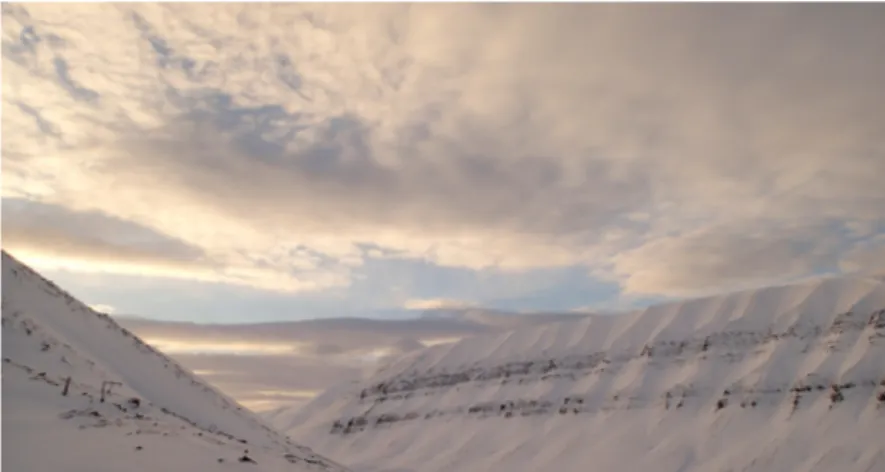
Figure 1.2: Stratus clouds that have developed in a mountainous region. Photo credit: Jan Chylík

Figure 1.3: A stratocumulus cloud, in the Arctic. Photo credit: Jan Chylík

classied as low level clouds. Boundary layer clouds make up a large portion of the cloud cover across the world, particularly over the ocean as shown in Fig. 1.1. Usually most low level clouds are made up of water droplets, but depending on the latitude and the temperature of the atmosphere where the cloud is present they can contain some ice crystals.

Boundary layer clouds include stratus, stratocumulus, and cumulus clouds and are dened by their formation and horizontal extent.

Stratus clouds, known for their sheet like features, are usually either white or gray in color, and are found in stratied air. One feature in stratus clouds that separates them from stratocumulus and cumulus clouds is the brous cloud base, meaning that the exact altitude of cloud base can be dicult to dene. Stratus clouds usually consist of water droplets, but on rare occasions can contain some ice crystals. In most cases these clouds do not precipitate, however under the right conditions it is possible that some drizzle is formed (American Meteorological Society, cited 2020a).

Similar to stratus clouds, stratocumulus clouds also very rarely produce precipitation. If

(13)

1.1 Boundary Layer Clouds

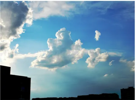
Figure 1.4: The detached and noticeable individual cumulus cloud, with the bright cloud top and a gray dark cloud base. Photo credit: Jan Chylík

precipitation is generated within the stratocumulus cloud it is usually in the form of drizzle.

Stratocumulus are often easily confused with stratus clouds, primarily due to their large- scale horizontal extent. However, there are a several dierences between the structures of these two clouds. Stratocumulus clouds are dened by their at cloud tops and non brous cloud base, which means that the cloud base is easier to determine compared to a brous cloud, and they also have a distinctive variation in color, with some of the patches being white while others are gray. While stratus clouds are dened by their continuous cloud sheet, stratocumulus is seen to have patches of clear sky surrounded by cloud (American Meteorological Society, cited 2020b). Stratocumulus clouds are the most common low-level cloud types seen across the world, with the average cloud cover over the ocean, between 1954 and 2008, being 22%and over land, between 1971 and 1996, being 12%(Hahn and Warren, 2007; Eastman et al., 2011).

While shallow cumulus clouds are relatively similar in structure to stratocumulus clouds, in that they have non-brous cloud edges. Unlike stratocumulus clouds, shallow cumulus clouds have a relatively small horizontal extent. Shallow cumulus clouds are dened by their tower like structures, which on occasion can begin to take the shape of a cauliower, with a bright white cloud top and a dark gray cloud base (Organization, 1975). Similar to stratus clouds, shallow cumulus clouds also have a diurnal cycle, which highly depends on whether the clouds are located above a land or ocean surface. Above land the maximum shallow cumulus cloud cover generally occurs in the afternoon, while over the ocean it generally occurs in early morning. Shallow cumulus clouds generally give an indica- tion of fair weather conditions (American Meteorological Society, cited 2020c). Following stratocumulus clouds, shallow cumulus are one of the most common low-level cloud types occurring over the ocean, with an average cloud fraction of 13%(Hahn and Warren, 2007;

Eastman et al., 2011). They are particularly common in the trade-wind regions above the oceans (Joseph and Cahalan, 1990; Cuijpers and Duynkerke, 1993; Johnson et al., 1999;

Bretherton et al., 2004; Siebert et al., 2013; Nuijens et al., 2014), e.g. o the west and northwest coasts of Barbados in the North Atlantic and o the coast of California in the Pacic.

(14)

1.2 Boundary Layer Clouds and Climate Change

Boundary layer clouds play an important role in the atmospheric conditions experienced.

The vertical structure of the boundary layer is highly dependent on the processes resulting in the formation of these boundary layer clouds. For a convective boundary layer the heat, humidity, and momentum are transported rapidly from the surface to higher altitudes in the atmosphere (Tiedtke et al., 1988; Cess et al., 1995; Siebesma et al., 2003; Zhao and Austin, 2005; Markowski, 2007; Siebert et al., 2013; Albrecht et al., 2019). These convective conditions can result in the formation of some boundary layer clouds such as shallow cumulus clouds and stratocumulus clouds. The formation of these clouds can then further drive convective conditions. The convective transport causes in the boundary layer deepen and as a result has an impact on the large-scale conditions, including the climate of the region.

Cloud parameters, such as cloud cover, have a strong inuence on not only the vertical structure of the boundary layer, but also on the Earth's radiation budget (Arking, 1991;

Albrecht et al., 1995; Nuijens et al., 2014; Bony et al., 2015). This eect on the radiative budget by boundary layer clouds is referred to as the cloud radiative eect (CRE).

Boundary layer clouds generally have a much higher albedo compared to the surface below them, this is particularly true for clouds over the oceans. Therefore the presence of boundary layer clouds can result in more solar radiation being reected which reduces the amount of heat reaching the surface, which would have a cooling eect on the boundary layer. Depending on whether the boundary layer clouds are shallow or deep, longwave radiation emitted by the surface can either be transported through the cloud into the free atmosphere, which results in a cooling eect on the boundary layer, or it can absorbed and re-emitted back towards the surface (Schneider et al., 1978; Hartmann et al., 1992), which would result in a warming of the boundary layer.

The resulting impact of the clouds on the radiation budget causes a feedback loop, referred to as the cloud feedback, in which the change in the radiation budget then has a corresponding impact on the boundary layer clouds. With a change in climate there would be a change in the radiation budget and therefore a corresponding change in the boundary layer clouds. It is however uncertain how these clouds will respond to this change in the radiation budget.

In future climates, it is expected that the atmospheric conditions will change, temperatures are expected to rise and a potential increase in the moisture at higher altitudes. This leads to a change in the boundary layer clouds, and as a result a corresponding change in the cloud feedback. The change in the cloud feedback would indicate whether the clouds have a warming or cooling eect on the boundary layer. It is therefore important to be able to correctly simulate this cloud feedback in predictions of future climates.

1.3 Project Aims

General circulation models (GCMs) have been used to simulate climate predictions, however large uncertainties have been seen between GCM models simulations, with dierent models simulating various dierent potential future climates. One of the largest uncertainties in these climate predictions is related to the feedback of boundary layer clouds to a change in climate (Bony and Dufresne, 2005; Boucher et al., 2013; Vial et al., 2013;

Blossey et al., 2016; Tan et al., 2016), in particular the feedback of marine boundary layer clouds. This uncertainty stems from the GCMs diculty in simulating boundary layer clouds, due to the horizontal extent of the boundary layer clouds being smaller than the

(15)

1.3 Project Aims

resolution of a GCM domain. Therefore the GCMs require parameterization schemes in order to simulate boundary layer clouds. Over the years, high resolution models, such as large-eddy simulation (LES) models, have been used to simulate proxy future climate simulations in an eort to understand this cloud feedback Klein et al. (2017). In these cases perturbations of increases in CO2 levels or sea surface temperatures have been used to gain an insight into how boundary layer clouds respond to a potential future climate.

This thesis investigates the possibility of using elevated moisture layers, which have already been observed in reality, as an additional method for studying how boundary layer clouds will respond to a change in climate, using an LES model. In order to investigate the response, it is rst important to understand the model and to determine how accurate the LES model is at representing observed conditions, before generating a simulation with an elevated moisture layer. The results from these simulations will focused on answering the question:

How do boundary layer clouds respond to a change in climate, using an elevated moisture layer as a proxy for a potential future climate?

The thesis is made up of 7 chapters which are divided between background theory, and the analysis of the simulations, rst focusing on determining the accuracy of the LES compared to observations, and then investigating the response of boundary layer clouds to an elevated moisture layer perturbation. Chapter 2 focuses on additional background theory of how boundary layer clouds form and their representation in observations and models. A detailed description of the observational campaign and model data used in the study is given in Chapter 3. Chapters 4 and 5 focus on comparing the LES model to the observational data, while Chapter 6 investigates the response of boundary layer clouds to the presence of an elevated moisture layer. Finally, the thesis concludes with Chapter 7 which includes the conclusions of the project and a future outlook.

(16)

Chapter 2

Boundary layer cloud formation and representation in observations and models

2.1 Formation of Boundary Layer Clouds

All clouds form when a parcel of air becomes saturated, which can occur as a result of increased moisture, decreasing temperature, or the introduction of mixing in the atmosphere, combined with available cloud condensation nuclei. As this air parcel rises through the boundary layer until it reaches its saturation level where it begins to cool and the water vapor begins to condensate onto cloud condensation nuclei, which consist of small aerosol particles (Seifert and Beheng, 2005). As the activated cloud droplets begin to grow they release latent heat. The manner in which these air parcels reach saturation dier between clouds, which in turn explains the general structure of the clouds seen in nature. Therefore the formation of a cloud is highly dependent on the atmospheric conditions in the region at the time of the cloud formation, which also include whether the boundary layer is in a stable or unstable state. Illustrative proles of the mean virtual potential temperature for the cloud free stable boundary layer and an unstable boundary layer can be seen in Fig.

2.1a) and b) respectively.

Stratus clouds are layered clouds that primarily form due to moist air advecting over a slightly cooler surface in a stable boundary layer. A change in the orography of the surface or an advection of colder drier air below the moist air is required to lift the saturated layer forming a stratus cloud. This can occur particularly at coastal regions when warm moist air is advected over a cooler land surface which is at a higher altitude, or over a plain covered by fog. It is also possible for stratus clouds to form as a result of the dissipation of fog. Based on the close connection between stratus clouds and fog a diurnal cycle of the stratus clouds is seen, with a maximum cloud cover occurring late at night and into the early morning (American Meteorological Society, cited 2020a).

Straocumulus clouds, also a layered cloud, form through dierent mechanisms compared to stratus clouds. While it is possible for a stratocumulus clouds to be present in either stable and unstable atmospheric boundary layer conditions, they do require some convection to form. This convection can act in several ways to produce a stratocumulus cloud. One method is by the convective transformation of a stratus cloud layer, resulting in the stratus cloud layer breaking up and patches of clear sky forming between cloudy regions. A second method, by which stratocumulus clouds can form, is by the convective lifting of a parcel

(17)

2.2 Observations of Boundary Layer Clouds

Figure 2.1: An illustration of the mean virtual potential temperature proles in a a) stable and b) unstable atmospheric boundary layer.

of moist air through an unstable boundary layer. When this rising parcel of air reaches a strong inversion, the cloudy air continues moving in horizontal directions.

Similar to stratocumulus clouds, cumulus clouds also require convection to form. This means that the atmospheric boundary layer is in an unstable state. If the a parcel of air at the surface is moist and warm enough, and thus less dense than the air around it, the convection in the atmosphere can cause it to lift. As the parcel of air begins to rise and continues to rise throughout the boundary layer it has a positive buoyancy. This release of latent heat increases the buoyancy of the air parcel (Lohmann et al., 2016) beyond the buoyancy of the air above the inversion, which allows the cloud to continue forming and increasing in altitude.

2.2 Observations of Boundary Layer Clouds

For over 50 years there have been numerous campaigns conduced to study the atmospheric conditions over the ocean. The aims of each of the individual observational campaigns conduced have varied, for example investigating interactions between the ocean surface and the atmosphere (Davidson, 1968), or studying the initiation and impact of precipitation in marine shallow cumulus clouds (Rauber et al., 2007b). The method of obtaining the observational measurements also varied from campaign to campaign, with several campaigns employing the use of instruments onboard research ships (e.g. Augstein et al., 1973), buoys, or instruments onboard aircrafts (Rauber et al., 2007b). Two of the pioneering campaigns, the Atlantic Tradewind Experiment (ATEX) (Augstein et al., 1973) and the Barbados Oceanographic and Meteorological Experiment (BOMEX) (Nitta and Esbensen, 1974), took place in 1969 and were both primarily based in tbe North Atlantic trade-wind region, where boundary layer clouds are a common feature as indicated in Fig. 1.1.

The ATEX campaign, which took place in February 1969, was divided into two observational periods. Through the rst period four research ships: Research Vessel Meteor, Research Vessel Planet, Research Vessel Discoverer, and the HMS Hydra, took part in the measurement campaign, while for the second period the HMS Hydra was not present. The three research vessels were positioned at the corners of an equilateral triangle and were

(18)

then allowed to drift along the ow of the trade winds. Throughout this period of observations there was very little precipitation present, with only one ship the Meteor observing a few showers of rain. The observations recorded during the ATEX campaign indicated that when the region has reduced convective activity and the trade-wind conditions are normally well developed a trade inversion develops which results in a separation between the divergent layer in the boundary layer and a convergent layer in the free troposphere (Augstein et al., 1973).

Several research ships took part in the BOMEX campaign, which was divided into four periods during May, June, and July of 1969. During this campaign a total of ve research ships: the Rainier, Mount Mitchell, Discoverer, and the Oceanographer were positioned at the corners of a square separated by 500 km, with the Rockaway located at the center of the square (Davidson, 1968; Kuettner and Holland, 1969; Holland, 1970; Holland and Rasmusson, 1973; Nitta and Esbensen, 1974). The BOMEX was not limited to a research ships. An aircraft ew around the perimeter of the square dened by the locations of the research ships. The main study of the BOMEX campaign investigated the dierences in the uxes in momentum, heat, and water vapor between the ocean and the atmosphere (Holland, 1970). Based on results from the campaign it was indicated that the uxes between the ocean and the atmosphere that were calculated, and the results of the subgrid- scale uxes, could be of benet in the development of eddy diusion coecients for models.

Overall it is stated that this campaign was a success.

Following the success of these pioneering campaigns, several additional campaigns took place in years between then and now. From June to September in 1974 a large campaign covering ocean and land stations took place as part of the Global Atmospheric Research Programme (GARP), the GARP Atlantic Tropical Experiment (GATE). This campaign made use of up to 39 ship based sites and 13 research aircrafts which generally ew from near Dakar out over the ocean towards the ship based sites in the region (Mason, 1975).

Studies based on this campaign included investigations into the fair weather boundary layer including boundary layer clouds (Nicholls and Lemone, 1980).

The focus on studying boundary layer clouds from observations continued with the inter- national Atlantic Stratocumulus Transition Experiment (ASTEX) (Albrecht et al., 1995).

The aim of the ASTEX campaign was to study and gain an understanding of the dierent processes that result in stratocumulus clouds transforming into a broken cloud. A second aim of the study was to investigate the processes that result in the formation of dierent types of clouds and the resulting cloud cover. It was aimed that the observations of these processes could lead to development of dierent parameterizations in models and also help with the development of the algorithms for satellites. The ASTEX campaign took place in June 1992 and was based o the coast of the Azores and Maderia Islands. A com- bination of measurements from aircrafts, ship, land based sites, and satellite were taken into account during the campaign. A vast dataset was obtained throughout the campaign, with approximately 600 soundings recorded during the campaign being assimilated into the ECMWF analyses data (Albrecht et al., 1995).

Since 2000, there has been an increase in the number of campaigns based in the tropical and subtropical trade wind regions. Between November 2004 and January 2005, the Rain in Shallow Cumulus over the Ocean (RICO) campaign was conducted o the coast of the Caribbean islands, primarily o the coast of Antigua and Barbuda. The primary reason for the development of the RICO campaign was to investigate atmospheric processes, based on observations, to study the initiation and development of precipitation. Observational measurements were recorded at four mobile sites: three research aircrafts and one research vessel, and one stationary site located at Spanish Point on the island of Barbuda. Each of the sites had several instruments in operation throughout the campaign. These instru-

(19)

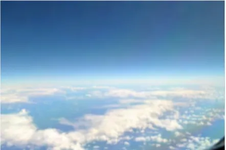
Figure 2.2: The convective clouds observed at 16:29 UTC during research ight 4 of the rst NARVAL campaign. Photo credit: Bjorn Stevens

ments included for example: several radar instruments recording at dierent wavelengths, radiosondes, lidars, cloud radars, and microwave radiometers. Additional information on the instruments and sites at which they were operated is given in Rauber et al. (2007a).

The RICO campaign was largely a success in that a large dataset was compiled giving insight into the development and level of precipitation produced in cumulus clouds within the trade-wind region. The datasets of observations recorded during the RICO campaign also give a base line for the conditions expected from weather and cloud resolving models (Rauber et al., 2007b).

Following the RICO campaign a permanent cloud observatory was constructed on the island of Barbados, the Barbados Cloud Observatory (BCO). The BCO consists of numerous instruments including an sky imager, water vapor DIAL, lidar, radiometer, two cloud radar, and a standard meteorological station to name a few (Stevens et al., 2016). The observations recorded at the BCO have complemented the more recent eld campaigns that have taken place since its construction, including the Clouds, Aerosol, Radiation and turbulence in the trade-wind regime over Barbados (CARRIBA) (Siebert et al., 2013), the two Next-generation Aircraft Remote-sensing for Validation (NARVAL) campaigns (Stevens et al., 2019a), and the ongoing Elucidating the role of clouds-circulation coupling in climate (EUREC⁴A) campaign (Bony et al., 2017).

As the observational dataset taken in to account in this study is from one of the research ights conducted during the rst NARVAL campaign, a detailed description is found in Section 3.1, where convective clouds such as the ones seen in Fig. 2.2 were observed.

Following the success of the rst NARVAL campaign, a second campaign was conducted during the wet season in August 2016. The High Altitude and Long-range research aircraft (HALO) was used as a remote-sensing platform in both NARVAL campaigns (Klepp et al., 2014; Stevens et al., 2019a). A large number of dropsondes were launched in a circle during two of the research ights in the second NARVAL campaign to test the potential for measuring the large-scale vertical velocity based on observations (Stevens et al., 2019a).

A total of 10 research ights took place as part of the second NARVAL campaign.

The work done as part of both NARVAL campaigns has been the building block for the currently ongoing EUREC⁴A campaign. The aims of the EUREC⁴A campaign are to study trade-wind cumulus clouds in relation to the large-scale conditions and to develop

(20)

2.3 Modeling Boundary layer clouds

a dataset that could be used to compare future simulations of cumulus conditions. The main measurement platforms for the EUREC⁴A campaign consist of 3 research aircrafts:

the German HALO aircraft, the French ATR-42, and the British Twin Otter aircraft, and 3 research vessels: the Maria S. Merian, the Meteor, and the L'Atalante (EURECA, 2020).

A corresponding campaign, the Atlantic Tradewind Ocean-Atmosphere Mesoscale Interac- tion Campaign (ATOMIC) (NOAA, 2020), from the National Oceanic and Atmospheric Administration (NOAA) is also being conducted as part of the EUREC⁴A. As part of the ATOMIC campaign, a fourth aircraft, the WP-3D aircraft, and a fourth ship, the Ronald H. Brown, are added to the EUREC⁴A campaign.

2.3 Modeling Boundary layer clouds

2.3.1 General Circulation Models

General circulation models (GCMs) allow for simulating the climate systems around the world, and in general can be useful for determining potential impacts as a result of climate change. Over the years there have been several GCMs developed with slightly dierent setups, however when predictions for future climate are generated a number of uncertainties into how the climate will change are seen. A large portion of these uncertainties have been associated with uncertainties in how boundary layer clouds will respond to a change in the climate (Bony and Dufresne, 2005; Boucher et al., 2013; Vial et al., 2013; Blossey et al., 2016; Tan et al., 2016, 2017). This is related not only to problems arising as boundary layer clouds, particularly shallow cumulus clouds, are generally only a fraction of the size compared to the dimension of the the GCM column, but there are also issues relating to the interactions and relationships between these clouds and the environment on a larger scale (Nuijens et al., 2014). As a result GCMs tend to have diculties in representing and determining the radiative eects of these clouds (Nuijens et al., 2014), the vertical structure of the boundary layer particularly when boundary layer clouds are present, and the general cloud fraction within the domain (McGibbon and Bretherton, 2017).

In order to take the boundary layer conditions and in particular the presence of boundary layer clouds into account, GCMs require parameterizations and will continue to require them in the near future (Siebesma et al., 2003; Abel and Shipway, 2007). These parameterizations were designed in order to represent the eects on boundary layer clouds on a subgrid scale (Betts, 1986). These parameterizations are generally divided into two main topics: 1) understanding the transport of moisture, heat, and momentum using a vertical turbulent mixing parameterization, and 2) a cloud parameterization (Siebesma et al., 2003). These can be then further divided, with the vertical turbulent mixing parameterization being subdivided into an eddy diusivity parameterization, a moist adjustment scheme, and a parameterization developed based on a mass ux scheme (Bretherton et al., 2004).

One of eddy diusivity schemes, that is applied in numerous GCMs and some single-column models, is described by Tiedtke et al. (1988). In an eddy diusivity scheme the sensible heat ux, the moisture turbulent ux, and the liquid cloud water are parameterized. This scheme takes into account the transport of the sensible heat and moisture, due to convection, within the cloud layer. Also within this particular scheme it is assumed that the eddy diusivity coecient is constant within an active cloud layer, while for passive cloud layers the eddy diusion coecient relies on the moisture distribution (Tiedtke et al., 1988).

A second common parameterization of the vertical transport in GCMs is the moist adjustment scheme approach. This parameterization is applied in an eort to reproduce the

(21)

moisture in the GCMs or large-scale models as realistically as possible. This method of parameterizing was proposed by Betts (1986) and then applied to datasets from a number of observational campaigns in Betts and Miller (1986). In this scheme the temperature and moisture structure is adjusted towards reference proles determined by the large-scale advective processes and the large-scale radiative processes. The cloud top is determined using a moist adiabat prole throughout the lower levels of the atmosphere, and therefore denes whether it is a shallow or deep convective system. For a shallow convective system the condensation, and therefore the precipitation, when integrated throughout the cloud layer, are zero. Therefore for shallow convection it is set that there is no precipitation. For deep convection however the reference proles are developed based on the total enthalpy.

Over the years there have been several dierent methods used to parameterize the liquid water in models and the cloud fraction in GCMs. Two methods of cloud parameterizations are a prognostic cloud scheme and a statistical cloud scheme. The prognostic scheme involves the inclusion of additional prognostic equations particularly for the cloud fraction and the liquid water. The statistical cloud scheme on the other hand is based on the potential to derive the values of the cloud fraction and liquid water. However this method only works if the subgrid scale values of the variability in both the temperature and the moisture are dened (Siebesma et al., 2003).

While the ability of parameterizations in GCMs have increased over the years, a number of weaknesses that contribute to the an uncertainty in climate prediction continue to exist (Bretherton, 2015). However there is hope that with the help of high resolution models, such as large-eddy simulation (LES) models, the understanding of the cloud eect can be expanded. While LES models do require some parameterization schemes, the variability on the subgrid scale is less complicated, as it is explicitly resolved. LES can also help with the developments and the evaluations of parameterization schemes that can be implemented into GCMs (e.g Siebesma and Holtslag, 1996; Siebesma et al., 2003; Neggers et al., 2009;

Matheou et al., 2011).

2.3.2 Large-Eddy Simulation Models

Since their application to atmospheric research over 50 years ago, LES models have been a huge benet in studying atmospheric processes, in particular boundary layer processes.

LES models are on a level between direct numerical simulations and GCMs, which means the methods they use are in between direct simulations of the turbulent ow and the results of Reynolds-averaging equations (Piomelli, 1999). As their name suggests LES have the ability to explicitly model larger turbulent eddies, while the small eddies in the turbulent cascade require parameterizations (Mason, 1994). Even though LES models do contain some parameterizations the dependence on these parameterization is to a much lower extent when compared to large-scale models such as GCMs (Heus et al., 2010).

Over the years, there have been several developments adding to the representation of processes in the lower troposphere including for example cloud microphysics (Seifert and Beheng, 2005), radiation, and the treatment of the surface. A variety of LES models have been developed over the years, for example the University of California Los Ange- les LES (UCLA-LES), the MetOce large-eddy model (MetOce LEM), the Icosahedral Nonhydrostatic LEM (ICON LEM), and the Dutch Atmospheric Large-Eddy Simulation (DALES) model. As DALES is used in this study a description of the model can be found in Chapter 3 Section 3.2.

LES models were initially used for gaining an understanding of the turbulent transport in the atmospheric boundary layer in studies by Lilly (1966), Deardor (1972b) and Deardor

(22)

(1972a). It was not long after these initial experiments, using LES models, that one of the rst studies on a boundary layer with clouds was conducted by Sommeria (1976). For the study by Sommeria (1976) the model described in Deardor (1972b) was used with slight modications.

Ever since these pioneering studies of boundary layer clouds, there have been numerous studies on the dierent aspects of the boundary layer conditions (Beare et al., 2006a), including boundary layer cloud types (e.g Cuijpers and Duynkerke, 1993; Brown et al., 2002). The LES models ability to reproduce boundary layer clouds has been tested by generating simulations over locations where observations have been recorded. These observations are based on either stationary observational measurement sites, such as Cabauw in the Netherlands (Schalkwijk et al., 2015) and the Atmospheric Radiation Measurement Southern Great Plains (ARM SGP) site (Zhang et al., 2017), or based on observational eld campaigns, such as BOMEX (e.g Siebesma and Cuijpers, 1995; Jiang and Cotton, 2000; Neggers et al., 2006) and RICO (vanZanten et al., 2011; Seifert and Heus, 2013).

These comparisons have given condence in the ability of LES in reproducing observed conditions, particularly with the developments on the microphysics schemes, which allow for the development of precipitation to be represented within the domain.

Intercomparison studies of LES models have been performed in order to compare dierent LES codes to each other and to observations, in order to determine the strengths and weaknesses of dierent LES codes in regards to representing observed conditions (Heus et al., 2010). There have been both large and small scale projects in this eld. Some of the larger general projects include studies completed under the Global Energy and Water Cycle Experiment's (GEWEX's) Atmospheric Boundary Layer Study (GABLS) (Beare et al., 2006b) and the GEWEX Cloud System Study (GCSS) (Duynkerke et al., 1999, 2004; Stevens et al., 2001; Siebesma et al., 2003; vanZanten et al., 2011).

In recent years some of the focus of LES studies have been directed towards studying the feedback from boundary layer clouds due to perturbations in the climate. These studies are divided between intercomparison studies, such as the Cloud Feedback Model Intercom- parison Project's (CFMIP) Global Atmospheric System Studies (GASS) Intercomparison of Large-Eddy and Single-Column Models (CGILS) (Blossey et al., 2013; Zhang et al., 2013; Blossey et al., 2016), and studies employing the use of a single LES model (e.g Xu et al., 2010; Rieck et al., 2012; Bretherton and Blossey, 2014). In each of these studies a perturbation is applied to a set of simulations. This perturbation is used to represent a potential future climate, e.g. an increased concentration of CO2 or an increase in the sea surface temperature.

(23)

Chapter 3

Observation and model datasets

3.1 Observations from the NARVAL Campaign

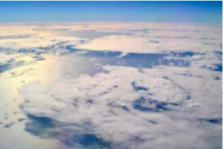
The main observational dataset used in this study is from the rst Next Generation Aircraft Remote-sensing for Validation (NARVAL) Campaign. The NARVAL Campaign made use of HALO, as an airborne remote-sensing platform. The main aim of the NARVAL Cam- paign was to investigate the shallow convection cloud structures and presence of clouds, like those seen in Fig. 2.2 and 3.1, and precipitation over two climate regimes in the North Atlantic, NARVAL South and NARVAL North. NARVAL South took place in December 2013 and was aimed at studying the trade wind regime in the North Atlantic, while NAR- VAL North took place in January 2014 and was aimed at studying winter mid-latitude storm-tracks. For both parts of the campaign, HALO was equipped with a specialized payload, including the microwave package, lidar, and the dropsonde system, along with several other instruments (Klepp et al., 2014). In the case of this study observations and retrievals from the dropsonde system and the HALO microwave package (HAMP) are used to determine the representativeness of the simulations. The measurements from the HAMP instrument and the additional instrumentation, such as the dropsonde system, made the overall NARVAL Campaign a success.

Figure 3.1: Convective clouds observed at 17:30 UTC during research ight 4 of the NARVAL campaign. Photo credit: Bjorn Stevens

(24)

3.1 Observations from the NARVAL Campaign

3.1.1 Dropsondes

The dropsonde measurements add to the HAMP data to give an insight into the thermodynamic conditions in the atmosphere during each research ight in the campaign. The dropsondes developed by Vaisala were launched from HALO at intervals throughout the ight, recording measurements of temperature, wind-speed, latitudes, longitudes, pressure, and the relative humidity throughout the atmosphere. The dropsonde system on board HALO during the campaign were global positioning system (GPS) dropsondes that were based on a dropwindsonde system described in Hock and Franklin (1999). The accuracy of these dropsonde measurements were relatively high with the pressure measurements accurate to within 0.5 mb, the relative humidity measurements had an accuracy of around 2 %, and wind speeds with an accuracy of 0.5 m s⁻¹ to 2.0 m s⁻¹ (Hock and Franklin, 1999). Throughout the entire campaign a total of 121 dropsondes were launched (Klepp et al., 2014).

3.1.2 HAMP

HAMP consists of three modules and is nadir pointing radiometer located in the bellypod of HALO. These three modules are divided into HALO KV, HALO 11990, and HALO 189.

HALO KV consists of two packages that are independent of each other for the K and V bands. HALO 11990 is also dived into two antennas independent of each other, a single detection retriever at 90 GHz and a signal heterodyne receiver which consisted of four channels ranging centered around the O2 line at 118 GHz. Finally HALO 189 consisted of a single heterodyne which retrieved signals over the H2O line centered on the 183 GHz line. Therefore in total, HAMP consists of 26 channels between 22 GHz and 195 GHz (Mech et al., 2014; Konow et al., 2018; Jacob et al., 2019). Using seven of the 26 HAMP channels, Jacob et al. (2019) was able to accurately retrieve values of IWV and LWP from the HAMP database.

3.1.3 Research Flights

A total of 13 research ights and two transfer ights were conducted over the North Atlantic during NARVAL. Eight of these research ights took place during NARVAL South and the remaining 5 research ights took place during NARVAL North. For NARVAL South four of the eight research ights were return trips between Oberpfaenhofen in Germany and Barbados, while the other four research ights were local ights out of Barbados. In three of the four local ights, the aircraft traveled more than half way across the Atlantic.

In this study, the focus is on research ight 4 which took place during NARVAL South.

While research ight 4 was a local ight, in that it left and returned to Barbados, it covered a large distance across the Atlantic. The ight track, shown in Fig. 3.2, shows that after leaving Barbados, HALO traveled approximately half way across the Atlantic to the location at which an overpass by CloudSat was performed. For this HALO turned and traveled south, before returning back to the original ight track and then back to Barbados. A total of 11 dropsondes were launched throughout the ight, the locations of which can be seen by the circles marked in Fig. 3.2.

During research ight 4, the large-scale thermodynamic conditions were generally homo- geneous, with some variations occurring at the beginning and ending of the ight. In the area around the Caribbean Islands a relatively deep convective system was present, which produced precipitation, during the day. This convection also resulted in the presence of a large humid layer at elevated altitudes of around 8 - 10 km. This elevated layer dissipated

(25)

3.2 The Dutch Atmospheric Large-Eddy Simulation Model (DALES)

Longitude [ ]

La tit ud e [ ]

5°N 15°N 25°N

79°W 64°W 49°W 34°W 19°W

Barbados

RF04 dropsondes

Figure 3.2: Flight track of research ight four, including the locations of each of the dropsondes that were launched throughout the ight. Modied version of the ight track to that seen in Klepp et al. (2014) and Reilly et al. (2019)

slightly as HALO traveled out across the Atlantic, where very dry conditions were observed above 2 km (Klepp et al., 2014). Upon returning to Barbados a deep convective system had developed resulting in an increase in the magnitude of the elevated humid layer and an increased depth of the boundary layer (Stevens et al., 2016).

3.2 The Dutch Atmospheric Large-Eddy Simulation Model (DALES)

This study makes use of the Dutch Atmospheric Large-Eddy Simulation (DALES) model.

The code for the DALES model, previously known at the KNMI large eddy simulation model, that is currently used is based on the model used by Wyngaard and Brost (1984) and Nieuwstadt and Brost (1986). The governing equations in DALES can be based on either the Boussinesq approximation, where the reference state variables are set to equal the value of the variables at the surface, or an anelastic approximation. The DALES setup used in this study uses the Boussinesq approximation for the governing equations.

Over the years DALES has been involved in many intercomparison studies investigating the representativeness of LES compared to observed conditions. Some of these intercom- parisons include simulations generated for observational campaigns such as the Atlantic Tradewide Experiment (ATEX) where DALES is referred to as the KNMI simulations (Stevens et al., 2001), and the Rain in Shallow Cumulus over the Ocean Campaign (RICO) (vanZanten et al., 2011). DALES is not however limited to intercomparison studies, it has also been used to study dierent atmospheric condition. These atmospheric conditions include convective boundary layers, which were rst studied using DALES by Cuijpers and Duynkerke (1993).

Over the years since the study by Cuijpers and Duynkerke (1993), DALES has beneted from its open source platform. Having the open source platform for DALES allows users to download, modify and exchange information on the code, depending on the research topics.

As a result of this DALES has been signicantly modied since the study by Cuijpers and Duynkerke (1993). Some of these modications are the inclusion of a number of schemes into the DALES setup, for example updated microphysics schemes and radiation schemes.

(26)

3.2.1 General Description of DALES

DALES requires at least three prognostic variables to be run, these are liquid water potential temperature (Θ_l), the velocity components, and the subgrid-scale turbulent kinetic energy (E) that are either calculated in the model or provided in the large-scale forcings.

Additional prognostic variables such as total water specic humidity (qt), rain droplet number concentration (Nr), and rain water specic humidity (qr), along with additional scalars can also be included (Heus et al., 2010). Large-scale forcing could also be applied for each prognostic variable with the exception of E.

3.2.2 Setup of DALES

One le required for using DALES is the namoptions le, which contains the settings for the simulations including the length of the simulation, the domain size and the resolution of the horizontal and vertical grids. Within the namoptions le it is also possible to set how often the large-scale eld is output as initialization proles, which allows the model to be rerun beginning at dierent time-points throughout the simulation using the warmstart function. Using the warmstart function can be benecial when running simulations with a large-domain and high resolution over a long time period, as it allows the simulation to be produced in smaller sections.

Forcing the LES back towards the large-scale state throughout the simulation, referred to nudging, can be applied to prevent drift in the model. This nudging, similar to the initialization and forcing of the LES, can be applied to either all prognostic variables, with the exception of E, that are provided by the large-scale variables, or individually specied prognostic variables. The nudging can also be applied over the entire prole or over a set range of altitudes. In order to switch nudging on in DALES, the ltestbed and ltb_nudge variables need to be set to true in the namoptions le. Following this the strength of the nudging (τ), referred to as tb_taunudge in the namoptions le, needs to be set to the length of time, in seconds, between the time-points at which DALES is nudged back to the large-scale reference state. The strength of the nudging is important, particularly when applying it to the entire prole, as when the nudging is too strong the turbulence in the boundary layer cannot develop. A detailed description of the nudging in DALES can be found in van Laar et al. (2019).

The DALES code uses a subgrid-scale scheme in order to determine the eddy diusivity coecients. Similar to the microphysics schemes, there are two main subgrid-scale schemes that can be employed by DALES. These subgrid-scale schemes are a sublter-scale turbulent kinetic energy (SFS-TKE) (Deardor, 1973) and the Smagorinsky schemes (Smagorin- sky, 1963). There are some similarities and dierences between the two subgrid-scale schemes in DALES. Both schemes use the three velocity component prognostic variables on a resolved case. There are however some dierences between the two schemes. While both schemes take into account the velocity component prognostic variables, the SFS- TKE subgrid-scale scheme also includes an additional prognostic equation which results in storing the prognostic variable of the subgrid turbulent kinetic energy. The Smagorinsky scheme on the other hand, does not include this prognostic equation. The Smagorinsky scheme does use the Smagorinsky theory which takes into account the stability and viscos- ity of the air.

3.2.3 Microphysics Scheme

There are two main microphysics schemes that can be employed by DALES, both of which are the bulk microphysics scheme. A bulk microphysics scheme is dened as a scheme in

(27)

which the drop size distributions follow a theoretical probability distribution. The droplet size distribution is assumed to follow a prescribed probability density function. The exact size distribution in each cell is then specied by values of the main moments, such as the mean. The two possible bulk microphysics schemes in DALES are the Khairoutinov and Kogan scheme (Khairoutdinov and Kogan, 2000) and the Seifert and Beheng two moment microcphysics scheme (Seifert and Beheng, 2001). The formation of rain is dependent on the type of microphysics scheme used for the individual simulations.

The scheme by Khairoutdinov and Kogan (2000) was developed for representing marine stratocumulus clouds in LES models. It was constructed based on results from a ne bin microphysics simulation (Heus et al., 2010). Within this microphysics scheme a series of prognostic variables are dened based on a number of settings, for example the initialization of cloud droplets is inuenced by the population of the cloud droplets. The droplet size is determined based on the the droplet concentration at specic liquid water content value.

While the Khairoutdinov and Kogan microphysics scheme is primarily used for stratocumulus cloud cases, the microphysics scheme by Seifert and Beheng (2001) and Seifert and Beheng (2005) is primarily for clouds which produce large amounts of precipitation. The microphysics scheme by Seifert and Beheng (2001) is developed by integrating the stochas- tic collection equation in order to determine the microphysical variables (Heus et al., 2010).

This microphysics scheme calculates autoconversion and accretion rates as the cloud begins to develop, and are used to ensure that the transformation of cloud water into rain water is considered.

3.2.4 Radiation Scheme

DALES can be run using dierent radiation calculations depending on the aim of the study.

The type of radiation calculation used is dened in the namoptions le before the simulation begins. There are ve main radiation calculations currently used in DALES. These are no radiation calculations, a parameterized radiation calculation, a full radiation calculation, a rapid radiative model, and a user dened radiation calculation. Switching o the radiation calculation in DALES also results in the diurnal cycle in the simulation being switched o as it is driven by the radiation scheme. For the user dened radiation calculation, the user modies one of the radiation fortran scripts before building the DALES code to be used in the simulation. The remaining radiation calculations, involves using two dierent radiation parameterization schemes, a longwave parameterization and a shortwave parameterization scheme.

The parameterization scheme for the longwave radiative transfer is the Global Energy and Water Cycle Experiment (GEWEX) Cloud System Study (GCSS) parameterization, which links the longwave radiative ux to the liquid water path. This is done using an analytic formula, which allows the simulation to be less computationally expensive (Larson et al., 2007). The shortwave radiative ux is calculated using the Delta-Eddington Model (Joseph et al., 1976). The Delta-Eddington Model calculates an asymmetrical phase function using a Dirac-delta function along side a two-term extension of a phase function (Joseph et al., 1976; Heus et al., 2010).

A rapid radiative transfer model has also been introduced to the DALES setup in recent years. This model also uses a Spectral Integration method, however it varies from the Monte Carlo Spectral Integration Model used by Pincus and Stevens (2009). Details of this rapid radiative transfer model are found in Mlawer et al. (1997). Finally, in the last 10 years, a fully interactive radiation scheme, the Monte Carlo Spectral Integration (Pincus and Stevens, 2009), has also been introduced into the DALES setup. This radiation model

(28)

3.3 Large-scale Forcing Dataset

is based on the k-distribution described in Fu and Liou (1992) and Fu et al. (1997). The benet of the full radiation scheme is that the radiative ux is determined for every grid point at each time-step in the LES. This radiative ux is calculated by either a part of a waveband where the absorption coecients are relatively similar, or by taking into account the full waveband that was randomly chosen. The use of the Monte Carlo Spectral Integration model for the full radiation scheme keeps computational costs reduced.

3.3 Large-scale Forcing Dataset

In order to run simulations using DALES, large-scale proles are required. These proles are used to initialize simulations and when required act as reference state proles towards which the LES can be nudged. Large-scale forcings can be derived from GCM output, on the condition that they contain the prognostic variables required by the LES. Two examples of GCM data from which the large-scale proles can be derived, are the Reanalysis and the Integrated Forecasting System (IFS) datasets from the European Center for Medium-range Weather Forecasts (ECMWF). The ECMWF Reanalysis dataset is a global dataset with information on the atmospheric conditions and surface conditions, and is produced as a result of running forecasting systems using observational data. The ECMWF IFS dataset on the other hand is forecast produced using an integrated computer software system.

These datasets have been used in many studies over the years, with ECMWF Reanalysis being used by Neggers et al. (2006) and Blossey et al. (2013). The ECMWF IFS dataset has been also used in several recent studies, for example studies by Neggers et al. (2012), Dal Gesso and Neggers (2018) and van Laar et al. (2019).

This study makes use of large-scale forcing proles derived from a ECMWF IFS dataset.

These large-scale forcings, derived from the IFS dataset, are based on 12 hour datasets that are complemented by short-range weather forecasts. This provides large-scale proles at a temporal resolution three hours. Having this temporal resolution of three hours, can be of benet particularly when nudging is applied by the LES back towards the large-scale forcings. DALES takes the proles of the atmospheric state variables, such as the total water specic humidity (qt), the liquid water potential temperature (Θ_l) and the wind velocity components in the u and v direction, into account when initializing, forcing, and applying nudging.

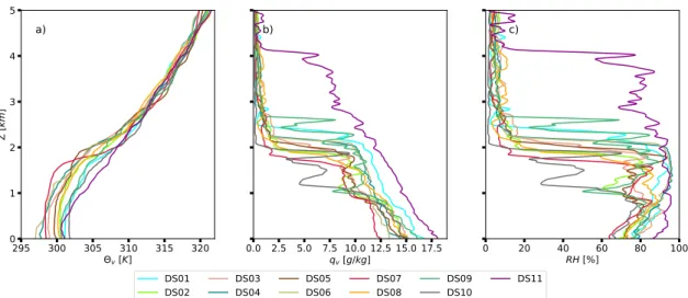
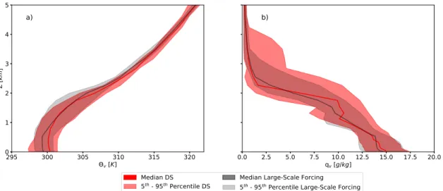
The proles of these atmospheric state variables are provided as averages over a 0.5 ^◦ x 0.5^◦ region around the area where the simulation is based. The vertical resolution of the derived large-scale forcing proles is relatively coarse. With a vertical height of 70 km and a total of 91 vertical levels, the vertical resolution decreases with increasing altitude. This means that the region of the atmosphere with the highest resolution is within the boundary layer. A detailed description of the large-scale forcings, similar to those used throughout this study, is given by van Laar et al. (2019).

Throughout this study, datasets derived from the ECMWF IFS model are used to initialize DALES and are used as reference proles towards which DALES is nudged either over the full atmospheric prole or over a range of altitudes above the boundary layer. Initially 11 large-scale forcing datasets where derived from ECMWF IFS output, for the regions around the locations of the 11 dropsondes launched during Research Flight 4 of NARVAL South. These datasets can be used to run individual simulations, as will be seen in Chapter 4, or run a composite case, as seen in Chapter 5 and Chapter 6.