GENETIC IDENTIFICATION OF SOURCE AND LIKELY VECTOR OF A WIDESPREAD MARINE INVADER Stacy A. Krueger-Hadfield

(1)

GENETIC IDENTIFICATION OF SOURCE AND LIKELY VECTOR OF A WIDESPREAD MARINE INVADER

Stacy A. Krueger-Hadfield^1,2*, Nicole M. Kollars^2†, Allan E. Strand², James E. Byers³, Sarah J. Shainker²,Ryuta Terada⁴,Thomas W.

Greig⁵,Mareike Hammann⁶, David C. Murray², Florian Weinberger⁶, Erik E. Sotka^2*

1 Department of Biology, University of Alabama at Birmingham, Birmingham, AL 35294-1170, USA

2 Grice Marine Laboratory and the Department of Biology, College of Charleston, 205 Fort Johnson Rd, Charleston, SC 29412.

3 Odum School of Ecology, University of Georgia, 130 E. Green St., Athens, GA 30602.

4 United Graduate School of Agricultural Sciences, Kagoshima University, Korimoto 1-21-24, Kagoshima City, 890-0065, Japan⁵ NOAA/National Ocean Service, Center for Coastal Environmental Health and Biomolecular Research, 219 Fort Johnson Rd, Charleston, SC 29312.

6 GEOMAR Helmholtz-Zentrum für Ozeanforschung Kiel, Düsternbrooker Weg 20, D-23105 Kiel, Germany.

*Corresponding authors: Stacy A. Krueger-Hadfield sakh@uab.edu; Erik E. Sotka eriksotka@gmail.com

†Current address: Center for Population Biology, University of California, Davis, CA, 95616.

(2)

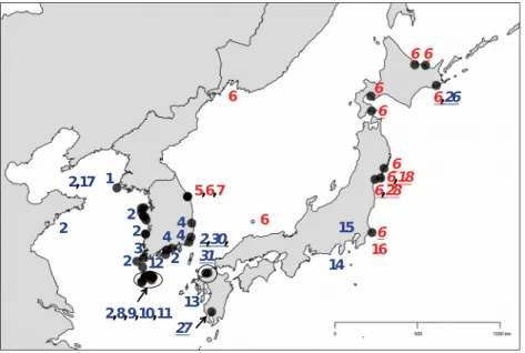
Figure S1. Mitochondrial cox1 haplotypic diversity from Kim et al., (2010) and this study. For maps and the tree, red and blue haplotypes have either a T or a C, respectively, at the 945^th bp. Sites sampled across the known distribution of Gracilaria

vermiculophylla: a) Native range, b) Non-native range west coast of North America, c) Non-native range east coast of the United States and d) Non-native range Europe and northern Africa. Haplotypes are shown next to the site in which they were sampled by Kim et al., (2010; shown in bold) and this study (shown in bold, italics and underlined). e) A phylogenetic tree of haplotypes from Kim et al., (2010) and this study. f) A 1.5% agarose gel with restriction enzyme products for six native non-source individuals from Odo-2-ri in Korea and Qingdao in China (C’s) and four individuals from Fort Johnson in the Charleston Harbor (T’s). These individuals were used as controls for all assays.

a)

2,17 1

2 2

2 23

12

2,8,9,10,11 2 4 44

5,6,7 6

27 13

2,30, 31

6 14

15 16

6,2866,18 6 6

6 6 6,26 6

(3)

b)

(4)

c)

(5)

d)

(6)

e)

(7)

f)

(8)

Table S2. a) The polymorphic sites across the 19 haplotypes from Kim et al., (2010) and the new haplotypes described in this study across the native and non-native ranges of Graclaria vermiculophylla. The SNP that differentiates the native source and non-source regions is shaded in gray. We used the haplotype numbers described by Kim et al., (2010), but not the ones described in Gulbransen et al., (2012). In the latter study, new haplotype numbers in Virginia were assigned based on aligning sequences across different studies and from sequences that did not span the entire length of the sequence (i.e., from 43F to 1549R). However, to avoid confusion with previously published haplotype numbers by Gulbransen et al., (2012), we have chosen different numbers for the six new haplotypes described here. Two of the Kim et al., (2010) haplotypes shared the same GenBank acc. Number (GU907106, see JPY_905_sm_TableS1-2). We called acc. GU907107 Haplotype 7 from Donghae (G530) and acc. GU907106 Haplotype 12 from Jeju (G510). b) The sites in this study for which cox1 was sequenced and the number of thalli at each site belonging to each haplotype.

(9)

a)

51 98 110 156 158 287 296 317 329 347 377 380 382 398 413 503 611

Haplotype 01 (GU907110)

T A C G C T T C C T C G C A A A C

Haplotype 02 (EF434936)

. . . . T . . . . . . . . . . . .

. . . . T . . . . . . . . . . G .

. . . . T C . . . . . . . G . . .

. . . . T A . . . . . . . G . . .

. . . . T . . . . . . . . G . . .

Haplotype 07 (GU907107)*

. . . . T . . . . . . . T G . . .

. . . A T . . T . . . . . G . . .

. . . . T . . . . . . T . . . . .

. . . . T . C . . . . . . . . . .

. . . . T . . . . . . . . . . . .

. . T . T . . . . . . . . . . . T

. . . . T . . T . . . . . G . . .

. . . . T . . . . . . . . G G . .

. . . . T . . . . C . . . . . . .

. . T . T . . . . . . . . G . . .

. . . . T . . . . . . . . G . . .

Haplotype 26 (KY621338)

. . . . T . . . T . A . . G . . .

. G . . T . . . . . . . . G G . .

. . . . T . . . . . . . . G . . .

C . . . T . . . . . . . . . . . .

. . . . T . . . . . . . . . . . .

(10)

629 638 677 767 770 860 866 917 945 947 989 1007 1031 1040 1106 1119 1154 Haplotype 01 (GU907110)

T T C C C T A T C A C T G C G A A

. . . . . . . . . . . . . . . . .

. . . . . C . . . G T . . . T . G

. . . . . . . . T . . . . T . . .

. . . . . C . . . . T . . . T C G

. . . . . . . . . . . . . . . . .

. . . . . . . . . . . . A . . . .

. . . . . . . . . . . . . . . . .

. . . . . C . . . . T . . . T . G

. . T . . C . . . . T . . . T . G

. . . . . C . . . . T . . . T . G

. . . . . . . . T . T . . T . . G

. . . . . . . . . . . . . . . . .

. . . . . . . . T . . . . T . . .

. . . . . . G . T . . . . T . . .

. C . T . . . . . . . . . . . . .

C . . . . C . . . . T . . . T . G

. . . . T . . . T . . . . T . . .

. . . . . . . . T . . C . T . . .

. . . . . . . . . . . . . . . . .

. . . . . . . C . . . . . . . . .

(11)

b)

Haplotypes Site 2 6 15 18 26 2

7 28 29 30 31

akk . 1

0 . . 3 . . . . .

fut . 7 . . . .

hik . . . 7 . . . .

hit . 6 . . . . 1 . . .

mn

g . 7 . 1 . . . .

mo

u . 1

1 . . . .

nag . 8 . . . .

shk 8 . . . .

shr . 8 . . . .

sar . 6 . . . .

usu . 9 . . . .

waj 2 . . . 5 1

bam . 4 3 . . . . 5 . .

bob . 7 . . . .

eld . 7 . . . .

mo

o . 7 . . . .

ptw . 7 . . . .

tmb . 7 . . . .

gar . 4 4 . . . .

lhp . 8 . . . .

mac . 5 1 . . . .

mag . 5 1 . . . .

nyc . 7 . . . .

ris . 8 . . . .

fme . 2 . 6 . . . .

frl . 4 . . . .

(12)

(13)

Figure S2. Discriminant analyses of principal components (DAPC). a) Cross-validation using the xvalDapc function as implemented in adegenet. The optimal number of principal components to retain was 88. b) Using the compoplot function as implemented in adegenet, we determined the a priori assignment of five subregions (native mtDNA-C, native mtDNA-T, WNA, EUSA and EU).

There was high a probability of assignment to these a priori clusters (92%). The y-axis shows the membership probability and along the x-axis are the 1670 diploid thalli genotyped. The majority of thalli were assigned to their cluster: native mtDNA-C (blue) had 94%

reassignment; native mtDNA-T (red) had 85.3% reassignment; WNA (purple) had 74.6.4% reassignment; EUSA (orange) had 97%

reassignment; EU (pink) had 92.3% reassignment.

(14)

a)

(15)

b)

(16)

Figure S3. a) The number of clusters inferred for the data set of diploid thalli including one copy of each genotype based on Psex. The DIC scores + SE for K=2 to K=30 using instruct. The mean similarity scores among different runs at the same K were computed using clumpak. The optimal number of clusters as determined by DIC was K = 23, but the mean similarity score was only 0.901. b-f) Cluster assignment as inferred by instruct and visualized using clumpak for optimal alignment of the 20 independent runs for different K’s.

The x-axis is arranged by site across the native range (divided into ‘C’ Haplotypes and ‘T’ Haplotypes) and the non-native range (divided into WNA, EUSA and EU). Each of the sites grouped together based on genetic similarity are shown by a dashed line along the x-axis (see Figure 3). b) K = 2. The mean similarity score was 0.995 and all 20 runs made up the major modes detected by clumpak. The y-axis shows the proportion of each site that belongs to a given genetic cluster. c) K = 3. The mean similarity score was 0.992 and 17 of the 20 runs made up the major modes detected by clumpak. d) K = 4. The mean similarity score was 0.990 and 18 of the 20 runs made up the major modes detected by clumpak. e) K = 5. The mean similarity score was 0.986 and all 20 runs made up the major modes detected by clumpak. f) K = 23. The mean similarity score was 0.901 and 19 of the 20 runs made up the major modes detected by clumpak. The site groupings based on genetic similarity shifted with the increased number of genetic clusters so that some sites that were previously grouped were no longer dominated by the same genetic cluster (e.g., dae and gye), whereas, other sites became genetically more similar (e.g., don, usu and jon).

(17)

a)

(18)

b)

(19)

(20)

c)

(21)

(22)

d)

(23)

(24)

e)

(25)

(26)

f)

(27)

(28)

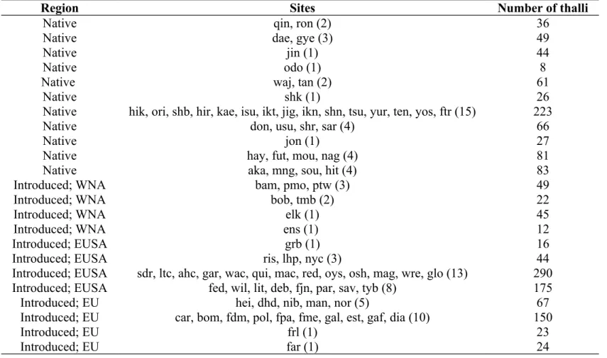
Table S3. The sample size of thalli and sites for the subregions used to calculate mean assignment to one of five genetic clusters identified using Bayesian clustering in instruct and visualized using clumpak.

Region Sites Number of thalli

Native qin, ron (2) 36

Native dae, gye (3) 49

Native jin (1) 44

Native odo (1) 8

Native waj, tan (2) 61

Native shk (1) 26

Native hik, ori, shb, hir, kae, isu, ikt, jig, ikn, shn, tsu, yur, ten, yos, ftr (15) 223

Native don, usu, shr, sar (4) 66

Native jon (1) 27

Native hay, fut, mou, nag (4) 81

Native aka, mng, sou, hit (4) 83

Introduced; WNA bam, pmo, ptw (3) 49

Introduced; WNA bob, tmb (2) 22

Introduced; WNA elk (1) 45

Introduced; WNA ens (1) 12

Introduced; EUSA grb (1) 16

Introduced; EUSA ris, lhp, nyc (3) 44

Introduced; EUSA sdr, ltc, ahc, gar, wac, qui, mac, red, oys, osh, mag, wre, glo (13) 290

Introduced; EUSA fed, wil, lit, deb, fjn, par, sav, tyb (8) 175

Introduced; EU hei, dhd, nib, man, nor (5) 67

Introduced; EU car, bom, fdm, pol, fpa, fme, gal, est, gaf, dia (10) 150

Introduced; EU frl (1) 23

Introduced; EU far (1) 24

(29)

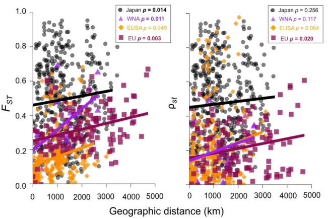
Figure S4. Genetic differentiation of Gracilaria vermiculopyhlla sites along the coastlines of native Japanese and non-native WNA, EUSA and EU coastlines. Pairwise genetic distances, measured by allele identity (FST) and allele size (ρST), are plotted against pairwise geographic distances (km) for each coastline. For pairwise FST, all slopes were significantly different from zero following sequential Bonferroni correction except for slope along the EUSA (significant p-values are shown in bold). In contrast, for pairwise ρST, only the slope along the EU coastline was significantly different from zero.

(30)

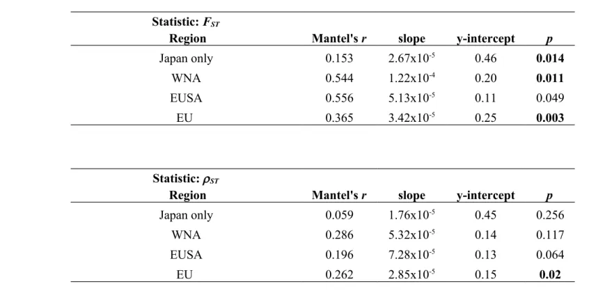
Table S4. Mantel’s r, slope, y intercept and p-value for Mantel tests across native and non-native coastlines for a) FST and b) ST as calculated using genpop. For allele identity, all slopes were significantly different from zero following sequential Bonferroni correction and are shown in bold except for the EUSA. For allele size, the only significant slope was the EU.

a)

Statistic: FST

Region Mantel's r slope y-intercept p

Japan only 0.153 2.67x10^-5 0.46 0.014

WNA 0.544 1.22x10^-4 0.20 0.011

EUSA 0.556 5.13x10^-5 0.11 0.049

EU 0.365 3.42x10^-5 0.25 0.003

b)

Statistic: ST

Region Mantel's r slope y-intercept p

Japan only 0.059 1.76x10^-5 0.45 0.256

WNA 0.286 5.32x10^-5 0.14 0.117

EUSA 0.196 7.28x10^-5 0.13 0.064

EU 0.262 2.85x10^-5 0.15 0.02

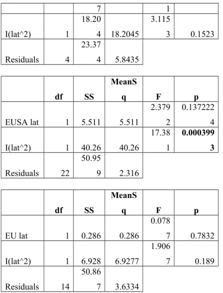
Table S5. ANOVA tables for each coastline and diversity metric. Significant p-values are shown in bold.

(31)

Response

: HE

df SS MeanSq F p

Native lat 1

0.00577 5

0.005775 2

0.649

3 0.426

I(lat^2) 1

0.00565 1

0.005651 3

0.635

4 0.4309 Residuals 34

0.30242 1

0.008894 7

WNA lat 1

0.04371

9 0.043719

11.81 2

0.0263 7 I(lat^2) 1

0.06176

5 0.061765

16.68 8

0.0150 4 Residuals 4

0.01480

5 0.003701

EUSA lat 1

0.00060 5

0.000604 9

0.148 8

0.7034 1 I(lat^2) 1

0.01424 3

0.014243 1

3.503 1

0.0746 1 Residuals 22 0.08945

0.004065 9

(32)

EU lat 1

0.00231 8

0.002318 2

0.388

7 0.543

I(lat^2) 1

0.00336 4

0.003364 4

0.564

1 0.4651 Residuals 14

0.08350 2

0.005964 4

Response

: AE

Native lat 1 0.0006 0.00055 0.0027 0.9586 I(lat^2) 1 0.0936

0.09363

4 0.465 0.4999 Residuals 34 6.8458

0.20134 7

WNA lat 1

0.6863

4 0.68634 4.943 0.09028 I(lat^2) 1

0.6653

4 0.66534 4.7918 0.09379 Residuals 4 0.5554 0.13885

EUSA lat 1 0.0784 0.07845 2.0266 0.1686

(33)

5 I(lat^2) 1

0.9593

6 0.95936

24.783 4

5.55E- 05 Residuals 22

0.8516

1 0.03871

EU lat 1 0.0871

0.08710

3 1.6473 0.2202 I(lat^2) 1

0.1462 1

0.14620

8 2.7651 0.1186 Residuals 14

0.7402 8

0.05287 7 Response

:

eML G

df SS

MeanS

q F p

Native lat 1 0.119 0.11912

0.048

1 0.8277

I(lat^2) 1 0.535 0.53474 0.216 0.6451

Residuals 34

84.17

5 2.47573

df SS

MeanS

q F p

WNA lat 1 11.50 11.5066 1.969 0.2332

(34)

7 1

I(lat^2) 1

18.20

4 18.2045

3.115

3 0.1523

Residuals 4

23.37

4 5.8435

df SS

MeanS

q F p

EUSA lat 1 5.511 5.511

2.379 2

0.137222 4

I(lat^2) 1 40.26 40.26

17.38 1

0.000399 3 Residuals 22

50.95

9 2.316

df SS

MeanS

q F p

EU lat 1 0.286 0.286

0.078

7 0.7832

I(lat^2) 1 6.928 6.9277

1.906

7 0.189

Residuals 14

50.86

7 3.6334

Figure S5. Bootstrapped (1000 replicates), unrooted neighbor-joining trees using sites with 10 or more thalli and jaccard distance for a) the native and non-native sites rooted in the native C site Qingdao (qin) and b) the non-native range alone rooted in the WNA site

(35)

Elkhorn Slough (elk). Few of the nodes in either tree had bootstrap support exceeding 0.5. The colors correspond to those used in the DAPC analyses where blue: ‘C’ haplotypes; red: ‘T’ haplotypes; purple: WNA; orange: EUSA; maroon: EU. Site codes can be found in Table S1.

a)

(36)

b)

(37)

(38)

Figure S6. Site assignment as inferred by DAPC using supplementary individuals as observations that did not participate in constructing the model. The supplementary individuals were predicted using a model fitted to other “training” data. The assigned sites are shown along the y-axis and the collected sites are shown along the x-axis. The probability of assignment to sites in the native range is shown with a heatmap ranging from white (0.0: no assignment) to black (1.0: complete assignment). As Eld’s Inlet had only one thallus after clones were removed, this site was removed from analyses. a) Native sites with >20% re-assignment of non-native thalli are shown in larger text and bold (**, mng had ~40% of non-native thalli assigned to it).

Native sites with 1% < x < 5% reassignment of non-native thalli are shown in smaller text.

Native sites with < 1% re-assignment are not shown on the map. b) WNA, EUSA and EU were each projected separately onto discriminant functions obtained from the native range the other two non-native coastlines. For example, the WNA sites were excluded from model construction.

Then, each of the WNA sites were projected on the discriminant functions constructed from the native range, EUSA and EU (hence, the “x” filling the cells along the assigned WNA sites as they could not be assigned to their own site or subregion). The probability of assignment is shown with a heatmap ranging from white (0.00: no assignment) to black (1.00: complete assignment). As Eld’s Inlet had only one thallus after clones were removed, this site was removed from analyses.

(39)

a)

(40)

b)