JO U R N A L O F PH Y S I C A L OC E A N O G R A P H Y
Freshwater in the ocean is not a useful parameter in climate research
URSULASCHAUER∗ANDMARTINLOSCH
Alfred-Wegener-Institut Helmholtz-Zentrum f¨ur Polar- und Meeresforschung
ABSTRACT
Ocean water is freshwater with salt. The distribution of salt concentration in the ocean changes by addition and removal of freshwater in the form of precipitation, continental runoff, and evaporation, and by a flow of saline ocean water that gives rise to a salt flux divergence. Often, changes in salinity are described in terms of “freshwater content” changes and oceanic “freshwater transports”, defined as fractions of freshwater. But these freshwater fractions are arbitrary, because they are defined by a non-unique reference salinity. Also all temporal and spatial comparisons and anomalies of such freshwater fractions in the ocean depend on the choice of reference salinity in a nonlinear way, because in the definition of the fraction it appears in the denominator. Consequently, any conclusion based on the comparison of freshwater fractions is ambiguous.
Since there is no definite physical constraint for a unique reference salinity, freshwater fractions are declared not useful for the assessment of the state of ocean regions and the associated changes. In the light of ongoing changes in the water cycle and the global nature of climate science, scientific results need to be expressed in a way so that they can be easily compared and integrated in a global perspective. To this end, we recommend to avoid freshwater fraction as a parameter describing the ocean state. Instead, one should use the terms of the salt budget to obtain unique results for quantifying and comparing salinity.
1. Introduction
Physical oceanography, like any other field of science, is based on measurable and derived quantities that can be compared to each other and to the respective terms of physical laws. To derive any understanding of processes and gain, for example, insight into the ocean’s role in the climate system, these comparisons need to be unambigu- ous. Here, by ambiguity we do not mean uncertainty due to instrumental errors, to non-synoptic observations, to in- terpolation, or to model resolution and parametrizations, but ambiguity due to an unavoidable arbitrary choice of reference. With ambiguous comparisons, also analyses and conclusions are ambiguous, and future scenarios can hardly be developed. As we will show, the concept of
“freshwater in the ocean” inevitably leads to this type of ambiguity and thus is not useful in physical oceanography.
Calculation of quantities that depend on an arbitrary ref- erence value yield arbitrary numbers by definition. Conse- quently, arbitrary parameters may cause considerable con- fusion if they come without clear specification through a name or a unit. For example, sound pressure level (loud- ness) is a parameter in acoustics, that needs a reference pressure. Since, for practical reasons, the reference pres- sure used in underwater acoustics is different from that
∗Corresponding author address: Alfred-Wegener-Institut Helmholtz-Zentrum f¨ur Polar- und Meeresforschung.
E-mail: ursula.schauer@awi.de
used in air acoustics, and even though these references are internationally accepted standards, misunderstandings easily appear evoking even societal debates (Finfer et al.
2008; Slabbekoorn et al. 2010).
The notion of freshwater in the ocean is mostly invoked in recognition of salinity changes being caused by dilu- tion or concentration due to adding or removing fresh- water. This exchange of freshwater is an important part of the hydrological cycle. In the non-oceanic compart- ments of the earth, soil, land-ice and atmosphere, freshwa- ter (which is simply termed “water” there) is an important quantity because the residence times, except for ice-sheets and glaciers, and the total amount of water are compara- tively small and changes of the water exchange are crucial.
In contrast, in the ocean the amount of water is large and changes are fairly small. But since these changes deter- mine the distribution of salt concentration, the freshwater flux into and out of the ocean has a huge impact on ocean processes.
Salinity itself is a key feature of the ocean. Together with temperature, it determines the density of ocean wa- ter and thereby influences almost all dynamical processes, ranging from the large-scale overturning circulation to double diffusive mixing at the centimeter scale. Salinity varies greatly in the world ocean, but this variability is not a consequence of sinks and sources of salt, as indicated by the small ratio between salt input (O(1012 kg/year)) and salt content in the ocean (O(1019 kg)), but of freshwater
Generated using v4.3.2 of the AMS LATEX template 1
(e.g. Talley et al. 2011). Precipitation, input from land by rivers, glaciers and groundwater, and loss by evaporation create large differences in salinity on various spatial and temporal scales. These salinity differences lead to ocean currents, but on the other hand, they are also subject to ocean currents as water masses with a surplus or a deficit of freshwater are transported to other regions.
In the first combined analysis of freshwater input and ocean salinities, Knudsen (1900) inferred the steady state ocean circulation between a partially enclosed basin and the adjacent ocean from salt and mass balances, including river runoff. This concept applies to any fixed volume of the ocean, also the global ocean (e.g. Talley 2008).
In the context of changes in the ocean, research also addresses changes of salinity. In the 1970s and 1980s, when large-scale salinity anomalies were first investigated they were still described as such, namely as “Great Salin- ity Anomalies” (Dickson et al. 1988; Belkin et al. 1998).
Only a few recent publications continue to provide salt budgets (Mauritzen et al. 2012; Treguier et al. 2014).
Since the 1990s, research papers often presented terms of a freshwater budget instead (e.g. Rahmstorf 1996; Ser- reze et al. 2006; Yang et al. 2016; Holliday et al. 2016, to give only a few examples). These terms are then called
“freshwater content” in the ocean as well as “freshwater transports”, for example through individual sections and gateways. Such ”freshwater content”Vffand ”freshwater transport”φffin the ocean is then defined as
Vff=VSref−S Sref
(1) and
φff= ZZ
sec
u⊥
Sref−S Sref
dl dz, (2) with an ocean volumeV with salinityS, and an arbitrar- ily chosen reference salinitySref. The double integral is evaluated over a vertical cross section area sec to which the velocity componentu⊥is perpendicular anddlanddz are the respective horizontal and the vertical line elements along the boundary.
The freshwater content of ocean water is, however, uniquely defined as
FW=1−10−3SA (3) withSAthe absolute salinity in g kg−1 (IOC, SCOR, and IAPSO 2010). This definition gives the mass relation, hence, the mass of freshwater in an ocean volumeV. The freshwater massVρFW (ρ for density) is comprising al- most the entire mass of ocean water.
Consequently, the parameters defined by eqs. (1) and (2) describe only fractions of the freshwater defined by eq. (3). Accordingly, we will call these terms “freshwater fraction” and “freshwater fraction transport” throughout this paper. This also differentiates the latter from “true”
freshwater inflow or removal through precipitation, evap- oration, and continental runoff. Note that Treguier et al.
(2014) suggested to use the terminology of “freshwater anomaly”, but we find “anomaly” misleading and also in- consistent with definition (3), because “anomaly” usually refers to a deviation from a mean.
Freshwater fractions first appeared in the context of re- gional analyses, but ultimately the nature of ocean and cli- mate science is global. This global nature requires that all analyses and results are formulated in a way that they can be integrated in a global perspective easily and seamlessly.
Results that depend on a locally determined reference can- not satisfy this requirement.
In one of the first publications on freshwater fraction transports, Aagaard and Carmack (1989) provided esti- mates of freshwater budgets of the Arctic Ocean and of the Nordic Seas. These budgets included the exchange between the two basins and with the North Pacific and the North Atlantic. Based on the same volume transports through the connecting passages Fram Strait and Barents Sea Opening and the same salinities in the passages, Aa- gaard and Carmack (1989) estimated different freshwater fraction transports depending on whether they calculated them for the Nordic Seas or for the Arctic Ocean because they based these transports on different reference salinities Sref. For example, they calculated the freshwater transport by southward flow in Fram Strait to be 820 km3yr−1and at the same time to be also 1160 km3yr−1. From a physical point of view, such an ambiguity of results is not accept- able because it does not allow closing an overall budget.
The root of the problem is the requirement of a reference salinity for computing the freshwater fraction terms.
Treguier et al. (2014) strongly recommended to use salinity in global analyses and to avoid analysing “fresh- water in the ocean” as defined by eqs. (1) and (2) as the results are ambiguous. To our knowledge, their study is the only one that avoids assessing freshwater fraction ex- plicitly for this reason. In this paper, we emphasize partic- ularly that freshwater fraction terms are not only ambigu- ous by themselves but, even more important, comparing them is ambiguous as well, because the reference value in the denominator determines also their differences. Since temporal or spatial comparisons or anomalies are the ratio- nale for any study, freshwater fraction cannot be a useful variable, neither on regional nor on global scales.
In this paper, we revisit the salt and volume budget (sec- tion 3) and stress that the relative change in ocean volume through addition or removal of pure fresh water is so small that in almost all cases this change can be neglected. Note that we will use the term “pure” freshwater for water that is supplied to the ocean from outside or leaving it. If the ocean volume remains constant and only the salt amount varies locally, all salinity changes can only be a conse- quence of a salt transport divergence. None of this is new.
For the stationary case, the salt and volume conserva- tion reduces to the concept of Knudsen (section 4). In sec- tion 5 we lay out the corresponding concept of freshwater fraction in the ocean and in section 6 we address how the spatial and temporal comparison of the different terms de- pends on the arbitrary choice of the reference salinity.
We discuss the question of a physical constraint for a particular reference salinity (section 7) that should be used, and, since there is no such constraint, whether it would be useful to seek an international binding agree- ment for such a reference (section 8). We strongly suggest in section 9 to use salt content, salt transport and changes thereof and to avoid all freshwater fraction terms because they are ambiguous and not physically convincing.
2. Data
We demonstrate the implications of the concept of freshwater fraction and the impact of the choice of ref- erence salinities in the context of the Arctic Ocean. The Arctic Ocean has a large input of pure (riverine and me- teoric) fresh water and at the same time various oceanic connections to the Pacific and the Atlantic. We use data of a very simple toy model of the Arctic Ocean that are inspired by data of the real Arctic Ocean. In addition, temporal changes of transports through passages between the Arctic Ocean and the Nordic Seas are addressed with simulations of a global configuration with an Arctic focus of the finite element sea-ice ocean model FESOM (Wek- erle et al. 2017). The advantage of using a toy ocean is that a closed salt and volume budget can be prescribed.
Also, basic insights are accessible more easily with a sim- ple model. In contrast, FESOM is sufficiently complex to mimic observational data with the additional advantage of no data gaps. Using observational data is not an alternative since the uncertainties due to a lack of representativeness of point measurements also lead to residuals in the salt and mass budget (e.g. Tsubouchi et al. 2018).
3. Conservation of salt and volume
As derived in numerous textbooks (e.g. Olbers et al.
2012) and publications (e.g. Wijffels et al. 1992), the salt budget of the ocean is controlled by the conservation laws of salt and mass of ocean water. Since sources of salt are negligible on the relatively short time scales of decades that are typical for physical oceanography, any change of salinity S in a fixed finite ocean volumeV can only be caused by a lateral diffusive and advective salt flux di- vergence through the enclosing fixed lateral boundaryA.
Neglecting the variability of density and the diffusive salt fluxes through the boundary, the conservation for the mass of saltsin the volumeVcan be written as
∂s
∂t =ρ I
∂A top
Z
bot
S u⊥dz dl (4)
withtfor time, andu⊥for the velocity normal to the verti- cal boundaryA. dzanddlare vertical and horizontal line elements. The sign convention makes inward fluxes pos- itive. The integration over the lateral boundary is written as an explicit vertical integration from bottom to top and a horizontal integration along the surface boundary∂Aof the enclosing vertical boundaryA. The salt transport di- vergence appears as a closed integral over the oceanic flow through the lateral boundaries, because there is no surface flux of salt.
A finite volume V of sea water can change by lat- eral transport through the boundaries and the flux of pure freshwater[P−E+R]through the surface:
∂V
∂t = I
∂A top
Z
bot
u⊥dz dl+ [P−E+R]. (5)
For convenience we have lumped all contributions to [P−E+R], the input from land through rivers, glaciers and groundwater R, the precipitation P, and the loss of freshwater through evaporationE, into a flux that can be thought of as a surface flux.
Today, a volume change from freshwater input on timescales of years to decades can only stem from the net mass loss of glaciers and ice sheets. Assuming an eustatic sea level rise of about 50 cm until the year 2100 (Stocker et al. 2013) this would be equivalent to an 0.15 permille increase of the ocean volume. The corresponding global mean salinity decrease would be 0.004 PSU which is at the limit of today’s measurement accuracy. Even a short local volume input such as the seasonal peak of river runoff into the Arctic Ocean (Haine et al. 2015) does not raise the sea surface over a substantial time because any surface pres- sure gradient resulting from the input immediately excites barotropic waves that remove the height difference within days to weeks (Treguier et al. 2014). Therefore, we can state that, for our purposes, the volume of an ocean re- gion can be considered constant, and the left hand side of eq. (5) can be neglected.
4. A steady state ocean with freshwater input - the Knudsen theorem
More than one hundred years ago, Knudsen (1900) used the conservation of mass and salt in steady state to de- rive estimates of the ocean circulation. Since then, the so-called Knudsen theorem (see the English translation in Burchard et al. 2018) has been widely used in estuarine re- search, for example, when river runoff and the salinities of inflow and outflow at the connecting ocean passages were used to infer the circulation and thus the flushing times of the estuary (Burchard et al. 2018). The Knudsen theorem can, however, also be applied to any ocean region when the inflow or evaporation of pure freshwater and the salin- ity along sections enclosing that region are known.
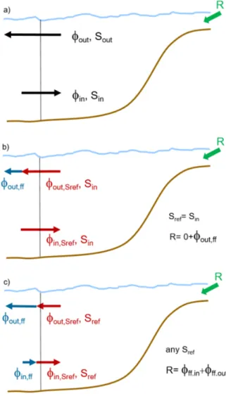
In a simple case, a river provides input of pure fresh- water to an estuary at a known rateR. This water mixes with saline water in the estuary and in steady state, saline water with a salinitySout leaves the estuary to the open ocean (Fig. 1a). To compensate the loss of salt and wa- ter, inflow of water withSin>Sout is required. The sub- scriptsinandoutindicate inflowing and outflowing water.
From conservation of salt (φinSin−φoutSout=0) and vol- ume (R+φin−φout=0), it follows that
R=φout
Sin−Sout
Sin
(6) in volume flux units, for example, Sv (1 Sv=106m3s−1).
Note that in the convention used here the transportφis al- ways positive, so thatφinincreases the volume and−φout
reduces the volume. From eq. (6) and withSin and Sout
known (e.g. measured), φout can be calculated and φin
can be computed from the difference betweenφout andR (Fig. 1a).
Note that Knudsen did not seek to trace “freshwater”
in the ocean, but the great step forward of his theorem was that it provided a simple method to make use of the information of pure freshwater input and relatively easy- to-obtain salinity values to quantify not-so-easy-to-obtain ocean transports. The theorem allows to derive these numbers in an unambiguous way. It was applied many times, for example to estimate the exchange in the Strait of Gibraltar (Nielsen 1912, and many others thereafter).
In a very elaborated way, Talley (2008) used the Knudsen principle to assess which parts of the global circulation match the pure freshwater flux divergences.
5. The concept of freshwater fraction in the ocean Despite the unique freshwater definition (IOC, SCOR, and IAPSO 2010, and eq. (3)), a plethora of publications (see section 1) use freshwater fraction terms and their changes with space and time to describe salinity changes.
Fig. 2 illustrates the general concept. Any volume of ocean waterV with a salinitySmay be considered as a composition of a fraction of freshwaterVff (subscript ff containing no salt and a fractionVSref with salinity Sref, henceV=Vff+VSref. The total amount of salt is then given byVSrefSref=V S. These two equalities can be combined into eq. (1)
Vff=VSref−S Sref .
This equation already illustrates the problem of the con- cept. Sref appears in the denominator so that the volume of freshwater Vff depends non-linearly on the reference salinity. This makes the definition fundamentally differ- ent from other physical quantities, including the TEOS10 freshwater definition of eq. (3).
FIG. 1. Sketch of an estuary with inflow of freshwaterR(green), outflow with salinitySoutand respective inflow with salinitySinacross a section denoted by the vertical line. a) shows the sketch in the sense of the Knudsen theorem where only the absolute flows are of interest;
in b) the outflow is split into a transport fraction with the salinitySin (red), and a fraction of freshwater transportφout.ff(blue); in c) the case is generalized to arbitrary reference salinities: both in- and outflow are split into a transport fraction with an arbitrary salinitySre fand a fraction of freshwater transport. Both flow fractions carrying salt (φin.Sref and φout.Sref) are of equal size and the combination of the freshwater flow fractionsφin.ff−φout.ffis alwaysR.
Within the concept of freshwater fraction transports in the ocean (eq. 2), the outflowφoutin eq. 6 and Fig. 1a can be seen as the combination of a flowφout.Sinexporting the salt that is imported byφin and that has the same salinity Sin (and thus equals φin) and a flow of freshwater φout.ff compensating the inflowR(Fig. 1b). Consequently,
φout.ff=φout
Sin−Sout
Sin
. (7)
FIG. 2. Illustration of a water column with a salinityS=34.8 that is interpreted as a combination of a column of salinitySrefand a column of freshwater, (a) for dilution, (b) for concentration.
In contrast to eq. (6), eq. (7) is equivalent to percievingSin
as a reference salinity for the flow of an oceanic freshwater fraction.
Eq. (7) can, however, also be formulated with any other arbitrary reference salinitySref (eq. 1). It then im- plies thatφout is composed of a respective saline φout.Sref
and freshwater flow fractionφout.ff. In this general case, also the inflowφin consists of respective fractionsφin.Sref
andφin.ff (Fig. 1c). Salt conservation requires again that φin.Sref=−φout.Sref, and volume conservation requires that φout.ff−φin.ff=R. In other words, in a steady state both the divergence of ocean currents and the divergence of flows of arbitrary freshwater fractions are equal to the pure freshwater input or output, no matter whichSrefwas used to defineφin.ffandφout.ffin terms of eq. (7) or, gener- ally, eq. (2).
VolumeVin Fig. 2 can also be interpreted as water with salinitySthat originates from a volumeVSref with salinity Sref, of which a certain amount of freshwater has been re- moved but the salt has been retained. The removed water has then been replaced by water withSref(Fig. 2b). Note that this description is equivalent to a salt transport diver- gence.
It is evident from eq. (1) that in any ocean volume the content of freshwater defined in this way depends as much on the observed salinity as on the reference salinity.
Accordingly, from a physical point of view, any volume of ocean water can be described containing a freshwater fraction ranging from large negative values to values ap- proaching 100%. In principle, anyone can arbitrarily de- cide how much freshwater is to be contained in a given sample of ocean water. Often, authors use mean values
of a basin (Aagaard and Carmack 1989) or along (set of) sections (Bacon et al. 2015).
6. The freshwater fraction budget
In section 5, we introduced the concept of artificially dividing a fixed ocean volume into a freshwater fraction and a fraction with the salinity Sref. For such an ocean volume, the budget can also be divided into one for the freshwater fraction and a second one for the water with salinitySref. Obviously, global conservation requires that the two budgets match.
The freshwater fraction budget is given through a bal- ance between the change of freshwater fraction content with time, the freshwater fraction transport divergence (a closed integral over the flow of freshwater fraction per- pendicular to the lateral boundary), and finally external sources and sinks:
∂Vff
∂t = I
∂A
Z top bot
u⊥,ffdz dl+ [P−E+R]. (8) To keep the total ocean volumeVconstant,
∂Vff
∂t +∂VSref
∂t =0,
there has to be a compensating exchange of water with the reference salinity. Thus, we get the second budget
∂VSref
∂t = I
∂V
u⊥,Srefda, (9) where now the closed integral means integration over the entire surface∂Vof volumeV. Eq. (9) makes clear that the concept of freshwater fraction repeats nothing else but that the salt content change is invoked by a salt flux divergence.
The flux divergence on the right hand side of eq. (8) may be composed of several individual branches through the lateral boundary and pure freshwater input. We show that comparing freshwater fraction transports across individual sections that do not form a closed boundary of a defined volume yields ambiguous results, not only for absolute values, but also for anomalies. Unfortunately, such com- parisons are made often (Tsubouchi et al. 2018; Schmidt and Send 2007, to name a few).
As shown above, the transports of freshwater fractions φffcan be derived as an expression analogous to that for the content; hence repeating eq. (2)
φff= ZZ
sec
u⊥
Sref−S Sref
dl dz.
Bothu⊥ andSvary withl andzand may also vary with time. Here, the section sec need not enclose a volume.
We will use the Arctic Ocean to illustrate the ambiguity of such freshwater fraction transports. The Arctic Ocean receives a huge amount of pure freshwater through the
rivers draining the North American and Eurasian catch- ments and therefore it is often regarded as a large estu- ary. It is however, connected to both the Pacific and the Atlantic Oceans through various passages. Pacific wa- ter with relatively low salinity (as compared to the Arc- tic Ocean mean salinity) and sea ice is imported through the Bering Strait; North Atlantic water with relatively high salinity is imported through the Fram Strait and the Bar- ents Sea Opening. Low salinity water and sea ice is ex- ported from the Arctic Ocean in the East Greenland Cur- rent and through the straits in the Canadian Archipelago.
The salinities of the outflows are determined by mixing and dynamics within the Arctic Ocean. The Bering Strait inflow is also considered a freshwater inflow because its salinity is low.
Often the freshwater fraction transports through the dif- ferent passages are calculated for the purpose of compar- ing them to each other and to the pure freshwater in- and outflow (Serreze et al. 2006). Some authors investigate, how the transports vary with time (Wekerle et al. 2013;
Rabe et al. 2013; Haine et al. 2015; Tsubouchi et al. 2018), and how much of a freshwater fraction is gained or lost by the Arctic Ocean (Rabe et al. 2014). In the following, we demonstrate that all results depend on the choice of refer- ence salinity.
a. Steady-state freshwater transports
In section 5, we mentioned in the context of the Knud- sen theorem that in steady state the sum of freshwater frac- tion transports equals the pure freshwater input. The indi- vidual transports, however, and, most importantly, their re- lation to each other depend on the choice ofSref. To illus- trate this, we use a simple toy model of the Arctic Ocean.
The values for the volume transports through the different passages and their bulk salinities are given at the bottom of Fig. 3. For simplicity, we combine here the Atlantic Water inflow through Fram Strait and Barents Sea Open- ing. Since we simulate an equilibrium case, the values of the in- and outflow transports and salinities are chosen in a way that the net input and output of volume and of salt are zero. Fig. 3 shows the freshwater fraction transports that enter or leave the Arctic Ocean based on different ref- erence salinities and that no clear judgement about neither their absolute nor their relative size can be made:
• For Sref=36 (a salinity typical for brine-enriched shelf water in winter) the freshwater fraction inputs through the Bering Strait inflow (rather low salinity) and the combined Fram Strait/Barents Sea Opening (WSCBSO) inflow (highest salinity of all inflows) are almost equal. Both are larger than the pure freshwa- ter inputφfffrom runoff etc. The freshwater fraction outflow is largest through the East Greenland Cur- rent (EGC) and the outflow through the passages of
FIG. 3. Freshwater transports by net pure freshwater inflow,[P−E+ R], and freshwater fraction fluxes through four oceanic gateways of a toy model of the Arctic Ocean based on differentSrefs (legend). Thex-axis shows the salinity (upper labels) and the volume flow (middle labels) of the gateways (lower labels). The gateway acronyms mean WSCBSO for the combined West Spitsbergen Current/Barents Sea Opening in- flow, and EGC for the outflow through the East Greenland Current. The salinities and transports are chosen in a way so that they are in equi- librium. The reference salinities are chosen as a fairly large (36) and a medium (34) value (see text), as salinity of the West Spitsbergen Cur- rent (WSC) (35), and the average salinity of all in and outflows in this configuration (33.38), following Bacon et al. (2015). Note that the sum of all oceanic freshwater transports for eachSref(each color) is equal and identical to P-E+R.
the Canadian Arctic Archipelago (CAA) is about two thirds of the EGC outflow.
• For Sref=35 (a typical Atlantic Water inflow salin- ity), the difference between the Bering Strait and the WSCBSO inflows is huge since the WSCBSO fresh- water fraction flow is now zero. While the Bering Strait inflow is again slightly larger than the pure freshwater input, the WSCBSO flow, being zero, is now much smaller than the runoff. The Canadian Archipelago outflow is now only about one third of the EGC outflow.
• For Sref=34 (a salinity typical for the lower halo- cline (Rabe et al. 2011)) the freshwater fraction flow through WSCBSO is negative, and in fact consid- erably so, namely more negative than the outflow through both outflow passages. The Bering Strait in- flow is now slightly smaller than the pure freshwater input, and the freshwater fraction transport through the Canadian Archipelago is even positive, that is, di- rected into the Arctic Ocean.
• For the boundary averaged salinity of 33.38, the
“only correct reference salinity” (Bacon et al. 2015),
the WSCBSO inflow provides now the largest neg- ative freshwater fraction contribution. Again, the Bering Strait inflow is positive but smaller than the runoff, however the second largest positive input is now provided through the Canadian Archipelago out- flow while the EGC outflow remains a freshwater fraction sink.
From this simple example we can easily see that al- most every combination of “main input contribution” ver- sus “smaller input” or of “strongest/weakest output” and inverse relations between inputs and outputs of freshwa- ter fractions can be obtained simply by the choice of reference salinity in a fairly moderate range of possi- ble ocean salinities. On the other hand, the associated salt transports are uniquely 0, 175, 31, −107, and −99 kt s−1 for [P−E+R], WSCBSO, Bering Strait, Cana- dian Archipelago, and EGC. Here, a constant density of 1000 kg m−3was assumed for simplicity.
Note also, that no information about the average salin- ity of the toy ocean is required neither for the freshwater fraction nor for the salt budget. The fact that each ocean is inhomogeneous with respect to salinity is the ultimate rea- son for having different outflow salinities (Dickson et al.
2007; Aagaard and Carmack 1989).
b. Time variability of freshwater fraction content and transports
One of the main goals in climate research is to consider non-stationary systems and to determine anomalies and the magnitude and direction of changes. Thus a consid- erable observational effort is directed to quantifying the variable content and transport of quantities in the ocean.
From eq. (1), we can see immediately how the choice of the reference salinitySrefinfluences not only the freshwa- ter fraction volumes themselves but also their difference
∆Vffwhen the salinity is changing fromS1toS2:
∆Vff=V
Sref−S2
Sref −Sref−S1 Sref
=VS1−S2 Sref For the example values in Table 1, the magnitude of the resulting ambiguities are of the order of 10% and more.
Note that the range ofSrefin Table 1 is approximately that of ocean salinities. From a physical point of view also much smaller or much larger Sref can be chosen, which would result in a larger ambiguity of a change in freshwa- ter fraction content.
The arbitrariness of comparisons of freshwater fraction contents or transports can also be seen in time series of the transport through a single passage (Fig. 4). Here we use results derived from FESOM simulations of velocities and salinities (Wekerle et al. 2017). From a 30 year time series in the East Greenland Current the liquid freshwater frac- tion export from the Arctic Ocean into the Nordic Seas is
TABLE1. Numerical example for the ambiguity in freshwater frac- tion content differences as a consequence of the choice of a reference salinity.
reference salinitySref 30 38
salinityS 34 35 34 35
freshwater contentVff(%) -13.33 -16.67 10.53 7.89 difference in freshwater
fraction content∆Vff(%)
-3.33 -2.63
FIG. 4. Anomaly of southward liquid freshwater fraction transports through the Fram Strait for different reference salinities. Salinity and volume transport data (see Fig. 5) from FESOM simulation (Wekerle et al. 2017; Horn 2019).
computed. Again, different reference salinities give very different absolute values (not shown). More relevant in the context of climate change research, the rates of change in the transport anomalies (Fig. 4) are different at almost any instance, and over many periods they do not even agree in the direction of change: during several phases, the fresh- water fraction export from the Arctic Ocean in the East Greenland Current has been both increasing and decreas- ing in the same time interval. It is entirely unclear how to use such information in the context of climate change research.
7. Are there physical constraints for a particular refer- ence salinity?
The ambiguity in the concept of freshwater fraction in the ocean, apparent in eq. (1), may be resolved if a univer- sal reference salinity could be derived from physical prin- ciples. We argue that there is no such universal reference salinity.
Common choices for reference include the mean salin- ity of an ocean volume (e.g. Aagaard and Carmack 1989;
de Steur et al. 2018), the “maximum salinity of inflow- ing water” (e.g. Dickson et al. 2007; Rabe et al. 2014), or the average salinity along the entire lateral boundary of a
given volume (Bacon et al. 2015; Tsubouchi et al. 2018).
Although all authors argue for their reference value, the different choices have in common that they change with time and also with the (adjacent) ocean basin. The fact that a basin or boundary average or transport maximum salinity changes with time makes these constant reference salinities incompatible with studying salinity change. In section 1, we discussed how different reference salinities for adjacent ocean basins immediately lead to conflicting values of “freshwater” flux through the connecting pas- sage.
The average salinity along the entire lateral boundary of a given volume was even claimed to be the only correct reference salinity (Bacon et al. 2015). Indeed, this choice does close the total budget of the freshwater fraction in the given volume – just as any other choice does. The proof of uniqueness in Bacon et al. (2015), however, is not convinc- ing because it is based on an inconsistent analogy. Further, in following the rule of Bacon et al. (2015) a neighbor ocean with a different boundary average salinity is again assigned a different reference salinity. Any passage con- necting the two adjacent oceans would then have two “cor- rect” reference salinities and thus two “unique” freshwater fluxes. If the different boundary meanSrefs were unique to specific ocean basins and regions, a combination of them to obtain global budgets would be impossible. This may serve as an independent indication that there cannot be a
“unique” or “correct”Sref.
8. Is it useful to seek an international agreement on a universal reference salinity?
In the absence of a plausible physical constraint for a reference salinity, it may be useful for the community to (1) agree on an internationally binding reference salinity and to (2) assign a special name and unit to the respective freshwater terms. In reflecting a few very general princi- ples of physical parameters, we discuss in the following, why such an effort is not worth consideration.
The measurement of a quantityQ, which is the first step in any metrological consideration, is just the comparison of the measured value with a standard, or reference. The used reference is expressed as the unit. The combination of a valuexand a unitb, for example distance relative to the unit meter, is unambiguously expressed as
Q=x·b. (10)
From the measured quantities, other quantities can be de- rived that are unambiguous as well. This quantity is abso- lute in the sense, that a value of zero implies that there is nothing of this quantity.
For example, length is an absolute parameter. It can be given in meters, inches, miles and other units. An identical length will then have different combinations of values and units. The key point is that also the difference between two
different lengths will be unambiguous through the unit:
∆Q=Q2−Q1= (x2−x1)·b, (11) while the ratio between two different lengths is even inde- pendent of units and thus of the reference system:
rQ=Q2 Q1 = x2
x1. (12)
Also salinity is an absolute parameter, that is, there is either no salt in the water, hence the salinity is zero, or there is some salt the concentration of which can be given in various units or no units, depending on which salinity is given (IOC, SCOR, and IAPSO 2010). These comparison principles hold for almost all parameters that are used to describe physics in a quantified way.
The other type of quantification is made relative to a ref- erence value that is chosen arbitrarily either since there is no absolute value (for example for potentials) or because of practical reasons. The most prominent example for a practical scale is temperature, for which the Celsius scale is used in daily life in most of the world and in Earth sys- tem science. The Celsius scale is based on an international agreement (Comit´e International des Poi Mesures 1969;
Preston-Thomas 1990) and it has its own unit, ◦C. The Celsius scale and the Fahrenheit scale, the other practical scale that is in use, are no longer absolute, because the linear relation between unit and parameter value includes now an offseta,
T=a+b·x. (13) A ratio between two temperatures,T1andT2, would there- fore have the form:
T1
T2 =a+b·x1
a+b·x2 (14)
and a statement like “temperature 1 is twice as large as temperature 2” cannot be made in the practical scales. It can be made for temperatures given in the Kelvin scale, for whicha=0.
Yet, any temperature difference is again well defined by the respective unit. Furthermore, the amount of heat (en- ergy) necessary to raise the temperature of a sample is in- dependent of the temperature scale because it is expressed by the temperaturedifferenceand two temperature differ- ences,∆Tnand∆Tm, can again be related unambiguously.
Consequently, the introduction of a practical scale for tem- perature with a reference offset is very meaningful and for all scales (Kelvin/Celsius or even Fahrenheit) the unit re- veals the value of the absolute values immediately.
For oceanic freshwater fraction terms, none of these principles hold. They have different values for different Srefbut the units (typically m3 for contents and mSv for transports) remain the same. Moreover, all comparisons depend on the choice of Sref, as is obvious from eq. (b)
FIG. 5. Time series of velocity weighted salinity (red) and vol- ume transport (blue, positive northward) of the southward flow in Fram Strait. Data based on the FESOM simulation (Wekerle et al. 2017; Horn 2019).
and Figures 3 and 4. Neither the difference nor the re- lation between freshwater fractions (content or transport) are independent of the reference salinity. Therefore, the oceanographic community should not strive to obtain an agreement on a universal reference salinity.
9. Return to salt and volume budget
We reviewed that the freshwater terminology does not help to explain ocean salt content, its changes, and oceanic transport variability, because, with the exception of pure freshwater, it is inherently ambiguous. To explain ocean salinity changes, we strongly recommend instead to return to the analysis of salinity and volume transports, and ulti- mately salt transports, considering that changes of the salt content in an ocean volume (i.e., changes of the volume average salinity) are a consequence of salt transport diver- gences (sections 3 and many oceanographic text books).
In contrast to freshwater fraction transports, salt transports are robust and unique absolute numbers.
As an incentive, consider the simulated freshwater transports in Fig. 4. They are based on time series of the southward volume transport through the Fram Strait and the respective transport-average salinity (Fig. 5). These time series immediately reveal two important features that cannot be seen from the freshwater plots: (i) there seems to be a correlation between volume transport and salinity with a weaker southward flow having a larger salinity and vice versa, and (ii) the range of variation is much larger for the volume flow (ca. 40% of the absolute value) than for salinity (0.3% of the absolute value).
The important budget term, however, is the salt trans- port. For the timeseries in Fig. 5, the salt transport vari- ation follows largely the volume transport variation and such a relation is probably true for most ocean transports.
FIG. 6. Salt transports in kt s−1through Fram Strait by the northward and southward flows (dashed lines, both drawn as positive flows) and the difference between the two (red solid line) resulting in a net salt transport that is directed northward.
This immediately suggests oceanographic interpretations of the flow that are otherwise obscured by the ambiguity of the relation between volume flow and freshwater flow.
No matter how small its salinity, the southward flow in Fram Strait exports salt from the Arctic Ocean and imports salt to the subarctic North Atlantic. While this salt trans- port is a robust number, it still does not say much about the contribution of this flow to salt content changes in either ocean since these changes are a consequence of the local salt transport divergence. To conserve volume, the large volume flow variation (Fig. 5) must be compensated and only in case of a salinity difference between the in- and the compensating outflows, the Arctic Ocean and North Atlantic will gain or lose salt. In the case of Fram Strait, a considerable part of the southward volume flow, including its variations, is balanced by the northward West Spits- bergen Current. Comparing the respective salt transports shows that an excess of 100 kt s−1 salt is carried north- wards (Fig. 6). The variations in the individual salt trans- ports, which are mostly induced by variations of the vol- ume transport, are largely compensated and do not show up in the net transport. What remains from the two op- posite flows is that the net salt import to the Arctic Ocean through Fram Strait has been smoothly increasing over the last 30 years (in this model simulation). Again, all salt transport time series, northward, southward and net salt transport through Fram Strait, yield themselves to imme- diate oceanographic interpretation.
There are a number of recent publications where the ambiguities of the freshwater terminology are avoided by quantifying the variation of salt content in a given ocean volume instead (e.g., Mauritzen et al. 2012) or by specifically quantifying salt transports instead of freshwa-
ter transports across latitudes (e.g., Treguier et al. 2014).
Jackson and Straneo (2016) computed salt transports to analyze ocean variability in a glacier fjord with pure fresh- water input through melting.
10. Conclusion
“Freshwater transport in the ocean can be a puzzling subject, with much confusion arising simply out of differ- ences in what is meant by the term freshwater transport.”
(Wijffels et al. 1992). After elucidating the meaning of the parameter “freshwater” in the ocean as an arbitrary fraction we conclude that not only “can” freshwater trans- ports within the ocean be puzzling, but rather they “are puzzling” by definition. We claim that, because of their arbitrariness, they are not useful for quantifying and un- derstanding ocean change.
The parameter “freshwater in the ocean” formulated as an arbitrary freshwater fraction cannot be used in any meaningful way because the results of comparisons and anomalies (both relations and differences) depend funda- mentally on the reference salinity. Comparisons, however, are the ultimate reason for any quantification.
Further, in the context of global changes, results from regional analyses, where for a short time a small com- munity of researchers may reach a local consensus on a particular reference value, need to be comparable between each other. This type of comparison is not possible with regionally defined freshwater fractions, either.
There are cases where certain types of freshwater in the ocean are of interest. For example, it is interesting to dis- criminate between glacial melt and meteoric water in the ocean and to trace the pathways of these waters. Such trac- ing can be uniquely achieved with source-specific tracers, such as oxygen isotopes (Bauch et al. 2016) or Helium (Huhn et al. 2018).
There is an increasing degree of arbitrariness in the use of ocean freshwater fraction:
i – In a stationary case or in climatological considera- tions, freshwater sources and sinks can be quanti- fied without any arbitrariness. They can be computed unambiguously as divergences of freshwater fraction transports (e.g. Talley 2008). The results are unique and independent ofSrefas pointed out by both Talley (2008) and Treguier et al. (2014).
ii – For all reference salinities, a freshwater fraction, of- ten called “freshwater content”, in a given volume will be larger for a lower salinity than for a higher salinity. However, the size of the difference depends on the reference salinity.
iii – For a freshwater fraction transport that is not mass balanced not even the sign is unique.
We emphasize that specifying freshwater fraction terms is not wrong in a physical sense. Fractions of freshwater
contents or transports with respect to a specifically chosen reference salinity are well defined, but this choice is only as valid as any other choice. Both mean values as well as anomalies of freshwater fraction transports are entirely ambiguous, including the sign of comparisons.
A fundamental misunderstanding already appears in the interpretation of “adding” or “removing” freshwater.
Adding pure freshwater to a region in the ocean does not result in a local volume change because of fast adjustment processes. Instead, the amount of salt changes because the added freshwater volume is compensated by an outflow of saline ocean water. Replacing saline water with pure freshwater is just a statement of salt flux divergence.
There is no physical constraint for a particular reference salinity and thus in the oceanographic literature, reference salinities are chosen in a suggestive and therefore subjec- tive way. Supposedly “correct” reference salinities (Bacon et al. 2015) turn out to be based on an inconsistent anal- ogy. It can be — and sometimes it is — argued that the dependence of the freshwater fraction terms on the differ- ent reference salinities in the oceanographic literature is not large, because the publishedSrefvalues do not differ very much. This reasoning resembles the joke about the drunkard seeking his lost key in the light cone of the street lantern, because in the darkness outside of the light cone he would not see it anyway. It is certainly not incorrect that similarSref lead to similar freshwater terms, but this insight is hardly a justification for dealing with arbitrary numbers. And it evokes immediately the question why there are different reference salinities in the first place.
The arbitrariness of freshwater budgets can easily be avoided (Treguier et al. 2014). Mass and salt conservation are unambiguous in both stationary and non-stationary cases. Salt transports through individual sections can un- ambiguously be compared since the mass of salt is an ab- solute quantity. Furthermore, salt budget terms have the profound advantage over freshwater fractions in that they lead more directly to oceanographical interpretation.
Salinity itself is a sophisticated quantity, which has been difficult to define (IOC, SCOR, and IAPSO 2010), and measuring it with high accuracy is difficult even to- day (Bud´eus 2011). Despite remaining caveats (Schmidt et al. 2018; Bud´eus 2018), practical salinity can be deter- mined as a unique parameter, and salinity changes can be analyzed by assessing salinity and ocean transports in a unique way, including the input of pure freshwater. It is entirely counter-productive to dilute the parameter salin- ity by watering it down with the artificial and ambiguous construction of “oceanic freshwater fraction”.
Acknowledgments. US was funded by the European Union’s Horizon 2020 research and innovation program under grant agreement H2020-BG-2014-2 (AtlantOS).
The authors are grateful to Sergey Danilov, Anne-Marie
Treguier and an anonymous reviewer for very helpful dis- cussion and comments.
References
Aagaard, K., and E. Carmack, 1989: The role of sea ice and other fresh- water in the Arctic circulation.J. Geophys. Res.,94 (C10), 14 485–
14 498, doi:10.1029/JC094iC10p14485.
Bacon, S., Y. Aksenov, S. Fawcett, and G. Madec, 2015: Arctic mass, freshwater and heat fluxes: Methods and modelled seasonal variabil- ity.Philos. Trans. Roy. Soc. London,373 (2052), doi:10.1098/rsta.
2014.0169.
Bauch, D., E. Cherniayskaia, and L. Timokhov, 2016: Shelf basin ex- change along the Siberian continental margin: Modification of At- lantic Water and Lower Halocline Water.Deep-Sea Res. I,115, 188–
198, doi:10.1016/j.dsr.2016.06.008.
Belkin, I. M., S. Levitus, J. Antonov, and S. A. Malmberg, 1998: “Great Salinity Anomalies” in the North Atlantic.Prog. Oceanogr.,41 (1), 1–68, doi:10.1016/S0079-6611(98)00015-9.
Bud´eus, G. T., 2011: Bringing laboratory salinometry to modern stan- dards.Sea Technology,52 (12), 45–48.
Bud´eus, G. T., 2018: Potential bias in TEOS10 density of sea water samples. Deep-Sea Res. I, 134, 41–47, doi:10.1016/j.dsr.
2018.02.005, URL http://www.sciencedirect.com/science/article/pii/
S0967063717300596.
Burchard, H., K. Bolding, R. Feistel, U. Graewe, K. Klingbeil, P. Mac- Cready, V. Mohrholz, L. Umlauf, and E. M. van der Lee, 2018:
The Knudsen theorem and the Total Exchange Flow analysis frame- work applied to the Baltic Sea.Prog. Oceanogr.,165, 268–286, doi:
10.1016/j.pocean.2018.04.004.
Comit´e International des Poi Mesures, 1969: The international practical temperature scale of 1968.Metrologia,5 (2), 35–44, doi:10.1088/
0026-1394/5/2/001, URL https://doi.org/10.1088%2F0026-1394%
2F5%2F2%2F001.
de Steur, L., C. PeraltaFerriz, and O. Pavlova, 2018: Freshwater export in the East Greenland Current freshens the North Atlantic.Geophys.
Res. Lett.,45 (13), 13 359 13 366, doi:10.1029/2018GL080207.
Dickson, R., B. Rudels, S. Dye, M. Karcher, J. Meincke, and I. Yashayaev, 2007: Current estimates of freshwater flux through Arctic and subarctic seas.Prog. Oceanogr.,73 (3–4), 210–230, doi:
10.1016/j.pocean.2006.12.003.
Dickson, R. R., J. Meincke, S. A. Malmberg, and A. J. Lee, 1988: The Great Salinity Anomaly in the northern North-Atlantic 1968-1982.
Prog. Oceanogr., 20 (2), 103–151, doi:10.1016/0079-6611(88) 90049-3.
Finfer, D. C., T. G. Leighton, and P. R. White, 2008: Issues relating to the use of a 61.5dB conversion factor when comparing airborne and underwater anthroprogenic noise levels.Applied Acoustics,69 (5), 464–471, doi:10.1016/j.apacoust.2007.05.008.
Haine, T. W. N., B. Curry, R. Gerdes, E. Hansen, M. Karcher, C. Lee, B. Rudels, G. Spreen, L. de Steur, K. D. Stewart, and R. Woodgate, 2015: Arctic freshwater export: Status, mechanisms, and prospects.
Global and Planetary Change,125, 13–35, doi:10.1016/j.gloplacha.
2014.11.013.
Holliday, N. P., S. Bacon, S. A. Cunningham, S. F. Gary, J. Karstensen, B. A. King, F. Li, and E. L. Mcdonagh, 2016: Subpolar North
Atlantic overturning and gyre-scale circulation in the summers of 2014 and 2016.J. Geophys. Res.,123 (7), 4538–4559, doi:10.1029/
2018JC013841.
Horn, M., 2019: Freshwater variability in the Arctic Ocean and subarc- tic North Atlantic. Ph.D. thesis, University of Bremen, 168 pp., URL https://elib.suub.uni-bremen.de/edocs/00106914-1.pdf.
Huhn, O., T. Hattermann, P. E. D. Davis, E. Dunker, H. H. Hellmer, K. W. Nicholls, S. Osterhus, M. Rhein, M. Schroeder, and J. Suel- tenfuss, 2018: Basal melt and freezing rates from first noble gas sam- ples beneath an ice shelf.Geophys. Res. Lett.,45 (16), 8455–8461, doi:10.1029/2018GL079706.
IOC, SCOR, and IAPSO, 2010: The international thermodynamic equa- tion of seawater - 2010: Calculations and use of thermodynamic properties. Tech. rep., Intergovernmental Oceanographic Commis- sion, Manuals and Guides No. 56, UNESCO (English), 196 pp.
Jackson, R. H., and F. Straneo, 2016: Heat, Salt, and Freshwater Bud- gets for a Glacial Fjord in Greenland.J. Phys. Oceanogr.,46 (9), 2735–2768, doi:10.1175/JPO-D-15-0134.1.
Knudsen, M., 1900: Ein hydrographischer Lehrsatz.Annalen der Hy- drographie und Maritimen Meteorologie, 28 (7), 316–320, URL www.scopus.com, in German.
Mauritzen, C., A. Melsom, and R. T. Sutton, 2012: Importance of density-compensated temperature change for deep North Atlantic Ocean heat uptake. Nature Geoscience,5 (12), 905–910, doi:10.
1038/NGEO1639.
Nielsen, J. N., 1912: Hydrography of the mediterranean and adjacent waters.Rep. Dan. Oceanogr. Exped. 1908-1910,1, 77–191.
Olbers, D., J. Willebrand, and C. Eden, 2012: Ocean Dy- namics. Springer, Berlin, Heidelberg, 708 pp., doi:10.1007/
978-3-642-23450-7.
Preston-Thomas, H., 1990: The international temperature scale of 1990 (its-90).Metrologia,27, 3–10.
Rabe, B., M. Karcher, U. Schauer, J. M. Toole, R. A. Krishfield, S. Pisarev, F. Kauker, R. Gerdes, and T. Kikuchi, 2011: An assess- ment of Arctic Ocean freshwater content changes from the 1990s to the 2006–2008 period.Deep-Sea Res. I,58 (2), 173–185, doi:
10.1016/j.dsr.2010.12.002.
Rabe, B., P. A. Dodd, E. Hansen, E. Falck, U. Schauer, A. Mackensen, A. Beszczynska-Moeller, G. Kattner, E. J. Rohling, and K. Cox, 2013: Liquid export of Arctic freshwater components through the Fram Strait 1998–2011.Ocean Science,9 (1), 91–109, doi:10.5194/
os-9-91-2013.
Rabe, B., M. Karcher, F. Kauker, U. Schauer, J. M. Toole, R. A. Krish- field, S. Pisarev, T. Kikuchi, and J. Su, 2014: Arctic Ocean basin liq- uid freshwater storage trend 1992-2012.Geophys. Res. Lett.,41 (3), 961–968, doi:10.1002/2013GL058121.
Rahmstorf, S., 1996: On the freshwater forcing and transport of the Atlantic thermohaline circulation.Climate Dyn.,12 (12), 799–811, doi:10.1007/s003820050144.
Schmidt, H., S. Seitz, E. Hassel, and H. Wolf, 2018: The density–
salinity relation of standard seawater.Ocean Science,14 (1), 15–40, doi:10.5194/os-14-15-2018, URL https://www.ocean-sci.net/14/15/
2018/.
Schmidt, S., and U. Send, 2007: Origin and composition of seasonal Labrador sea freshwater.J. Phys. Oceanogr.,37 (6), 1445–1454, doi:
10.1175/JPO3065.1.
Serreze, M. C., A. P. Barrett, A. G. Slater, R. A. Woodgate, K. Aagaard, R. B. Lammers, M. Steele, R. Moritz, M. Meredith, and C. M. Lee, 2006: The large-scale freshwater cycle of the Arctic.J. Geophys.
Res.,111 (C11), doi:10.1029/2005JC003424.
Slabbekoorn, H., N. Bouton, I. van Opzeeland, A. Coers, C. ten Cate, and A. N. Popper, 2010: A noisy spring: the impact of globally ris- ing underwater sound levels on fish.Trends in ecology & evolution, 25 (7), 419–427, doi:10.1016/j.tree.2010.04.005.
Stocker, T. F., D. Qin, G.-K. Plattner, M. Tignor, S. K. Allen, J. Boschung, A. Nauels, Y. Xia, V. Bex, and P. M. Midgley, Eds., 2013: Climate Change 2013: The Physical Science Basis. Contri- bution of Working Group I to the Fifth Assessment Report of the In- tergovernmental Panel on Climate Change. Cambridge University Press, Cambridge, United Kingdom and New York, NY, USA, 1535 pp.
Talley, L. D., 2008: Freshwater transport estimates and the global overturning circulation: Shallow, deep and throughflow compo- nents. Prog. Oceanogr., 78 (4), 257–303, doi:10.1016/j.pocean.
2008.05.001, URL http://www.sciencedirect.com/science/article/pii/
S0079661108001080.
Talley, L. D., G. L. Pickard, W. J. Emery, and J. H. Swift, 2011:De- scriptive Physical Oceanography: An Introduction. sixth ed., Else- vier, 560 pp.
Treguier, A. M., J. Deshayes, J. Le Sommer, C. Lique, G. Madec, T. Penduff, J. M. Molines, B. Barnier, R. Bourdalle-Badie, and
C. Talandier, 2014: Meridional transport of salt in the global ocean from an eddy-resolving model.Ocean Science,10 (2), 243–255, doi:
10.5194/os-10-243-2014.
Tsubouchi, T., S. Bacon, Y. Aksenov, A. C. N. Garabato, A. Beszczynska-Moller, E. Hansen, L. de Steur, B. Curry, and C. M.
Lee, 2018: The Arctic Ocean seasonal cycles of heat and freshwa- ter fluxes: Observation-based inverse estimates.J. Phys. Oceanogr., 48 (9), 2029–2055, doi:10.1175/JPO-D-17-0239.1.
Wekerle, C., Q. Wang, S. Danilov, T. Jung, and J. Schr¨oter, 2013: The Canadian Arctic Archipelago throughflow in a multiresolution global model: Model assessment and the driving mechanism of interannual variability.J. Geophys. Res.,118 (9), 4525–4541, doi:10.1002/jgrc.
20330.
Wekerle, C., Q. Wang, W.-J. von Appen, S. Danilov, V. Schourup- Kristensen, and T. Jung, 2017: Eddy-resolving simulation of the Atlantic Water circulation in the Fram Strait with focus on the sea- sonal cycle.J. Geophys. Res.,122 (11), 8385–8405, doi:10.1002/
2017JC012974.
Wijffels, S. E., R. W. Schmitt, H. L. Bryden, and A. Stige- brandt, 1992: Transport of fresh-water by the oceans. J.
Phys. Oceanogr., 22 (2), 155–162, doi:10.1175/1520-0485(1992) 022h0155:TOFBTOi2.0.CO;2.
Yang, Q., T. H. Dixon, P. G. Myers, J. Bonin, D. Chambers, M. R.
Van den Broeke, M. H. Ribergaard, and J. Mortensen, 2016: Re- cent increases in Arctic freshwater flux affects Labrador Sea convec- tion and Atlantic overturning circulation.Nature Communications, 7 (10525), doi:10.1038/ncomms10525.