Adaptive Order FlowForecasting withMultiplicativeError Models

S F B

XXX

E C O N O M I C

R I S K

B E R L I N

SFB 649 Discussion Paper 2014-035

Adaptive Order Flow Forecasting with

Multiplicative Error Models

Wolfgang K. Härdle*

Andrija Mihoci*

Christopher Hian-Ann Ting**

* Humboldt-Universität zu Berlin, Germany

** School of Business Singapore Management University, Singapore

This research was supported by the Deutsche

Forschungsgemeinschaft through the SFB 649 "Economic Risk".

http://sfb649.wiwi.hu-berlin.de ISSN 1860-5664

SFB 649, Humboldt-Universität zu Berlin Spandauer Straße 1, D-10178 Berlin

SFB

6 4 9

E C O N O M I C

R I S K

B E R L I N

Adaptive Order Flow Forecasting with Multiplicative Error Models ^∗

Wolfgang K. Härdle

, Andrija Mihoci

and Christopher Hian-Ann Ting

Abstract

A flexible statistical approach for the analysis of time-varying dynamics of transaction data on financial markets is here applied to intra-day trading strategies. A local adap- tive technique is used to successfully predict financial time series, i.e., the buyer and the seller-initiated trading volumes and the order flow dynamics. Analysing order flow series and its information content of mini Nikkei 225 index futures traded at the Osaka Securities Exchange in 2012 and 2013, a data-driven optimal length of local windows up to approxi- mately 1-2 hours is reasonable to capture parameter variations and is suitable for short-term prediction. Our proposed trading strategies achieve statistical arbitrage opportunities and are therefore beneficial for quantitative finance practice.

JEL classification: C41, C51, C53, G12, G17

Keywords: multiplicative error models, trading volume, order flow, forecasting

∗Financial support from the Deutsche Forschungsgemeinschaft via CRC 649 ”Economic Risk” and IRTG 1792 ”High Dimensional Non Stationary Time Series”, Humboldt-Universität zu Berlin, is grate- fully acknowledged.

†Humboldt-Universität zu Berlin, C.A.S.E. - Center for Applied Statistics and Economics, Spandauer Str. 1, 10178 Berlin, Germany and School of Business, Singapore Management University, 50 Stamford Road, Singapore 178899

‡Humboldt-Universität zu Berlin, C.A.S.E. - Center for Applied Statistics and Economics, Spandauer Str. 1, 10178 Berlin, Germany, tel: +49 (0)30 2093 5728, fax: +49 (0)30 2093 5649

§School of Business Singapore Management University, 50 Stamford Road, Singapore 178899

1 Introduction

Modelling and short-term forecasting of transaction data has become an important goal in academia and in practice. While understanding high-frequency dynamics, researchers suggest more accurate modelling solutions and provide more precise out-of-sample fore- casting results. A successful application in intra-day trading practice similarly demands carefully chosen trading strategies and financial solutions at any trading minute during the trading hours at a securities exchange.

This paper introduces a flexible framework for an useful data-driven application of time- varying dynamics for retrieving valuable information from transaction data at financial markets. The proposed financial steps and trading execution strategies start by employing the the so-called local adaptive multiplicative error models by Härdle et al. (2014) due to their demonstrated predictive accuracy. In adaptive forecasting of aggregate trading volume series these models statistically outperform benchmark models. Here we use them to meet the demands of business practice as we discuss the information content of the volume and the order flow series dynamics as well as the temporary imbalance between buy and sell orders. Our paper thus contributes to the financial and banking literature, as the dynamics of several (key) high-frequency financial time series is carefully analysed and successfully applied in intra-day trading.

The modelling and the forecasting part of our study integrates the local parametric ap- proach originally proposed by Spokoiny (1998) and themultiplicative error models intro- duced by Engle (2002) and therefore accommodates time-varying parameters, see, e.g., Härdle et al. (2014). From statistical perspective, in (volume and order flow) time series modelling, longer data intervals induce a large modelling bias and shorter ones lead to quite volatile parameters. The aim is here to strike a balance between the bias and the (in)efficiency at each point in time while finding an estimation window with potentially varying length, the so-called interval of homogeneity, in which one can safely assume a parametric multiplicative error model (with constant parameters) to hold. This is done

by a sequential testing procedure and the resulting intervals are used in our study for prediction and the performance evaluation of competing trading strategies.

Order flow dynamics provides valuable information for inferring the direction of price moves, as documented in recent literature. Although trading activity is generally consid- ered to be important and informative, its measurement is still contentious in the litera- ture. For example, Jones et al. (1994) show that the positive relation between volume and price moves is due to the number of trades and not the transaction size. They con- clude that volume has no information content beyond that which is already impounded in the number of transactions. On the contrary, Chan and Fong (2000) and Chordia et al.

(2002) find that trade size is more significant in explaining the volume-volatility relation, particularly when it is employed to measure the aggregate order flow between buyer- and seller-initiated trades. Moreover, Chordia et al. (2001) and Cairney and Swisher (2004)’s papers highlight the importance of order flow as a measure of trading activity. Their re- sults demonstrate that order flow is more valuable than volume in inferring the direction of price moves for the next trading day. The implication of this finding in the context of designing trading strategies that yield anomalous returns is obvious.

Adaptive order flow modelling is suitable for understanding of the imbalances in trades initiated by market orders at transaction level. Order flow or order imbalance makes sense, strictly speaking, when there is a middleman to make the market by holding an inventory to accommodate temporary imbalance between buy and sell orders. For a fully automated exchange that has no designated market maker, there is no order flow in the sense of inventory management. As the underlying construct of order flow is trade direction, one could still entertain order flow for trades executed by a computer. A market order that hits a limit order at the ask price could be considered as buyer-initiated, and seller-initiated trades are those executed at bid prices. The imbalance in trades initiated by market orders is then defined analogously as the difference between those that hit the ask and those that hit the bid. It is of our outmost interest to employ trading strategies based on the predicted imbalances in trades.

In summary, our paper’s objectives include short-term order flow forecasting and intra-day trading. Adaptive order flow modelling provides a sound framework for the prediction of transaction data. While employing numerous intra-day trading strategies, our method- ology provides valuable insides into the dynamics of imbalances in trades initiated by market orders for inferring the direction of price moves and represents a basic building block in securities trading.

The remainder of the paper is structured as follows. After the data description in Section 2, the local adaptive multiplicative error model framework is introduced in Section 3.

Empirical results concerning the modelling and the forecasting of the order flow series are provided in Sections 4 and 5. Section 6 concludes.

2 Data

In adaptive order flow time series forecasting we focus on the high-frequency dynamics of mini Nikkei 225 index future contracts due to the availability of the intra-day data. Our data originate from the Osaka Securities Exchange, where mini Nikkei 225 index futures are actively traded in the regular session from 9:00 till 15:10 Japan time (UTC+9:00).

The contract size (also known as the price multiplier) of this futures contract is U100, and the minimum tick size is 5 index points. The contract months follow a quarterly cycle: Mar (H), Jun (M), Sep (U), and Dec (Z). The last trading day is the business day preceding the second Friday of each contract month, whereas the final settlement day is the business day preceding the second Friday of each contract month.

Our main data service provider is Bloomberg, which assigns the ticker symbol NO to the mini Nikkei 225 index futures traded exclusively at the Osaka Securities Exchange. We obtain the records of each trade and every best quote that enter into Bloomberg’s ticker plant through the Excel API. The data fields are Date and Time, Type (whether it is bid, ask or trade), Size (number of contracts), Condition Codes, and Exchange Code.

Our sample period is from 28 June 2012 to 24 May 2013. We analyse the following series:

i. NO12U: 28 June - 13 September 2012 ii. NO12Z: 14 September - 13 December 2012 iii. NO13H: 14 December 2012 - 7 March 2013, and iv. NO13M: 8 March - 24 May 2013.

The chronologically arranged data records allow us to infer the trade direction of each trade. We check the best bid and the best ask price prior to each trade. If a trade occurs at the ask price, it is classified as buyer-initiated trade, and the volume traded is called the buyer-initiated volume. Conversely, if a trade occurs at the bid price, it is labelled as seller-initiated trade, and seller-initiated volume accordingly. Data on 4 March 2013 are excluded because the trading stopped between 11:06 and 14:10, as well as the data after 15:00 at all trading days to avoid the large price swings that typically occur during market closing. In total, our high-frequency tick data span 218 trading days, and each day starts from 09:01 to 15:00.

We use 1 minute as the time interval to aggregate the buyer- and seller-initiated volumes.

The 1-minute (absolute) order flow is computed as the aggregate buyer-initiated volume minus the seller-initiated volume. The relative order flow equals the ratio between the buyer-initiated volume to the aggregate volume. Over the sample period, a total of 78,480 minutes of observed order flows are obtained.

We denote the one-minute cumulated buyer-initiated volumes at day d and minutei by

˘

y^b_i,d. Similarly, the seller-initiated volume are notated by ˘y^s_i,d. The price data includes the ask S_d,i^a , the bid S_d,i^b and the transaction price S_d,i at beginning of minute i.

Trading volume data displays an intraday pattern. To account for the intraday peri- odicity effects we follow econometric literature and use a Flexible Fourier Series (FFS) approximation, see, Gallant (1981). The seasonally adjusted volumes are given by

9 11 13 15 0

2 4

Factor

NO12Z

9 11 13 15

0 2 4

NO13H

9 11 13 15

0 2 4

NO13M

9 11 13 15

0 2 4

Factor

Trading Hour 09 11 13 15

2 4

Trading Hour

9 11 13 15

0 2 4

Trading Hour

x10³ x10³

x10³

x10³ x10³ x10³

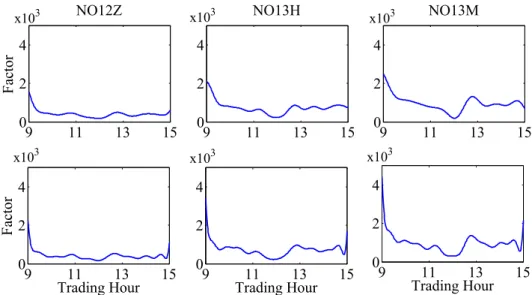
Figure 1: Estimated intraday periodicity factors for the buyer-initiated (upper panel) and the seller-initiated (lower panel) trades for the ’mini Nikkei 225 index futures’ traded at the Osaka Securities Exchange on 13 December 2012 (NO12Z), 7 March 2013 (NO13H) and 24 May 2013 (NO13M)

- Buyer-initiated volume, y^b_i,d = ˘y^b_i,d/s^b_i,d−1 - Seller-initiated volume, y^s_i,d = ˘y_i,d^s /s^s_i,d−1

ford= 31, . . . ,218 (13 August 2012 - 24 May 2015), i= 1, . . . ,360 with periodicity com- ponent si,d−1 at minute i and day d. The later are estimated based on a 30-day rolling window basis, see, e.g., Engle and Rangel (2008). Consider (s1,d−30, . . . , s360,d−1)^> and

si,d−1 =δ¯ı_i+

M

X

m=1

{δ_c,mcos (¯ı_i·2πm) +δ_s,msin (¯ı_i ·2πm)}

where ¯ı = (¯ı₁, . . . ,¯ı₃₆₀)^> = (1/360, . . . ,360/360)^> denotes the intraday time trend. The estimated periodicity factors for the volume series on the last days of the NO12Z, NO13H and NO13M series (13 December 2012, 7 March 2013 and 24 May 2013) are displayed on Figure 1.

The estimated intraday periodicity factors for the buyer- and the seller-initiated volumes, reveal typical intraday trading patterns: the volume is relatively high during the opening hours and during the closing period. Less contracts are traded during midday phase.

3 Local Adaptive Multiplicative Error Models

In financial econometrics it is a challenging task to understand the trading volume and the order flow dynamics. Local adaptive multiplicative error models are used for analysing and forecasting of high-frequency time series, see Härdle et al. (2014). Their framework employs the local parametric approach (LPA) originally proposed by Spokoiny (1998) to the multiplicative error models (MEM) introduced by Engle (2002). The underlying idea is to find an estimation window, the so-called interval of homogeneity, in which one can safely fit a parametric multiplicative error model with constant parameters. Since the methodology accounts for time-varying MEM parameters and because it selects data- driven estimation windows here we use it for high-frequency time series forecasting.

3.1 Multiplicative Error Models

The multiplicative error model by Engle (2002) plays an important role in the analysis of positive valued financial market data, such as trading volumes, durations, bid-ask spreads or price volatilities. In high-frequency financial data modelling Engle and Russell (1998) used a special type of a MEM, i.e., the so-calledautoregressive conditional duration (ACD) model, see a comprehensive MEM literature overview by Hautsch (2012).

The MEM models a non-negative valued time series, denoted byy={y_i}ⁿ_i=1, as a product between its conditional mean µ_i and an unit mean positive valued error term ε_i

yi =µiεi, E[εi| Fi−1] = 1 (1)

conditional on the information setF_iup to observationi. The conditional meanµ_ifollows an ARMA-type specification

µ_i =µ_i(θ) =ω+

p

X

j=1

α_jyi−j+

q

X

j=1

β_jµi−j (2)

with parameter θ = (ω, α^>, β^>)^> where α = (α₁, . . . , α_p)^> and β = (β₁, . . . , β_q)^> col-

lect the parameters associated with lagged observations of the process and its lagged conditional mean, respectively.

Motivated by econometric literature we assume that the error term follows a (standard) exponential distribution and thus focus on theExponential-ACD(EACD) model, see, e.g., Engle and Russell (1998) and Härdle et al. (2014). By utilising the (quasi) maximum likelihood estimation, the (quasi) log-likelihood function over a (right-end) fixed interval I = (i0−n, i0 ] ofn observations at time pointi0 is given by

`_I(y;θ) =

n

X

i=max(p,q)+1

−logµ_i− y_i µi

!

I{i∈I} (3)

where I{•} denotes the indicator function. The (quasi) maximum likelihood estimate over interval I is then given by

θe_I = arg max

θ∈Θ `_I(y;θ). (4)

3.2 Local Adaptive Multiplicative Error Models

In modelling trading volume and order flow series we utilise the local adaptive multi- plicative error model framework by Härdle et al. (2014) to meet the quantitative practice demands. A data-driven approach in parameter estimation and hypothesis testing is pro- posed with the focus on the selection of reasonable (tuning) parameter constellations for each of the analysed high-frequency series. It is therefore expected that our empirical results provide valuable insides into high-frequency dynamics. This part describes the statistical modelling background while empirical evidence is provided in Section 4.

There are four basic steps in the application of the local adaptive multiplicative error models. The statistical framework part discusses the underlying idea and introduces the statistical background. A detailed description of the so-called local change point detection test and the resulting testing procedure enable us to determine the interval of

homogeneity. The adaptive estimation part finally defines the adaptive estimate, that is used in further analysis, particularly in forecasting time series and in intra-day trading.

Statistical Framework

Including more observations in an estimation window enlarges the modelling bias and reduces the variability of the estimate. The key idea is therefore to strike a balance be- tween the modelling bias and the parameter variability, which can be accomplished by approximating the ’true’ model by a parametric model with constant parameters over a

’relatively short’ time interval. This local parametric approach has been originally pro- posed Spokoiny (1998) and since then it has been gradually introduced into econometric time series literature. For an application to daily data, including exchange rates, index returns and stock index returns, see, e.g., Mercurio and Spokoiny (2004), Čížek et al.

(2009) and Chen et al. (2010). The study by Härdle et al. (2014) applied the framework to the high-frequency volume series.

The proposed framework covers the case of time-varying coefficients that are either smooth functions of time or that are modelled as piecewise constant functions of time.

Parameters can thus vary over time as the interval changes and can account for discon- tinuities and jumps as a function of time. The quality of the local approximation is theoretically measured by the Kullback-Leibler divergence and in practice a sequential testing procedure is developed to determine the ’optimal’ window. The later procedure helps us to find the so-calledinterval of homogeneity at any fixed time pointi0. It is thus safe to assume the (multiplicative error) model to hold over the resulting interval.

The data intervals used in the sequential testing procedure includeK+ 1 nested intervals with fixed right-end point i₀, i.e., Ik = [i₀−nk, i₀] of length nk, I₀ ⊂I₁ ⊂ · · · ⊂IK. The lengths of the underlying intervals are assumed to evolve on a geometric grid with initial length n0 and a multiplier c > 1, such that nk =^hn0c^ki. Here a suitable selection of the initial lengthn0 and the multiplier cis based on empirical results provided in Section 4.

Based on the test outcome at fixed time point i0, one of these K + 1 intervals will then

be regarded as the interval of homogeneity. In the sequel the interval of homogeneity is used for short-term adaptive forecasting of the order flow series.

Local Change Point Detection Test

Searching for the interval of homogeneity among the K+ 1 interval candidates is based on a sequential procedure, i.e., the local change point detection test is constructed as a sequential test. The null H₀ of the test at step k means that the (interval) sequence up to I_k is homogeneous. The alternative hypothesis H₁ states that there exists a change point within I_k. Note that here we are not interested in the change point(s) position(s) per se, i.e., we are searching if there exists a change point at all within the investigated data intervalIk or not.

By assuming that the intervalI₀ is homogeneous, the test statistics at the first step (i.e., testing MEM parameter homogeneity over I₁) is given by

T₁ = sup

τ∈J₁

n`<sub>A1,τ</sub>θ<sup>e</sup><sub>A1,τ</sub>+`_B1,τ θ^e_B1,τ−`_I2θ^e_I2^o, (5)

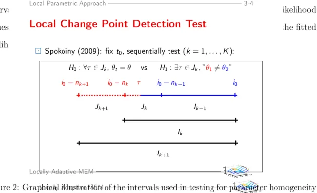
with intervalsJ₁ =I₁\I₀,A_1,τ = [i₀−n₂, τ] andB_1,τ = (τ, i₀] that use only a part of the observations withinI₂. As the location of the change point is unknown, the test statistic considers the supremum of the corresponding likelihood ratio statistics over all τ ∈J₁. The calculation of the test statistic at step k is conducted similarly as at the first step, and the procedure is illustrated in Figure 2. By assuming that the null of parameter homogeneity at step k−1 has been established, the test statistic equals

T_k = sup

τ∈J_k

n`<sub>Ak,τ</sub> θ<sup>e</sup><sub>Ak,τ</sub>+`_Bk,τθ^e_Bk,τ−`_Ik+1θ^e_Ik+1^o. (6)

Data from the interval I_k+1 have been similarly used to determine the intervals J_k = I_k \Ik−1, A_k,τ = [i₀−n_k+1, τ] (coloured red in Figure 2) and B_k,τ = (τ, i₀] (coloured blue in Figure 2), whereas the test statistic considers the supremum of the corresponding likelihood ratio statistics over allτ ∈J_k. While testing for parameter homogeneity of the

intervalI_k, one considers the supremum over all points τ of the sum of the log likelihood values over the intervals A_k,τ = [i₀−n_k+1, τ] and B_k,τ = (τ, i₀] in relation to the fitted likelihood for data withinI_k+1 ranging from i₀ toi₀−n_k+1.

Local Parametric Approach 3-5

Frame

Local Parametric Approach 3-4

Local Change Point Detection Test

Spokoiny (2009): x t₀, sequentially test (k =1, . . . ,K):

H0:∀τ ∈Jk,θ_t =θ vs. H1:∃τ ∈Jk, θ₁6=θ₂ i₀−n_k+1 i₀−n_k τ i₀−n_k−1 i₀

J_k+1 J_k I_k−1

Ik

Ik+1

Locally Adaptive MEM

0.700.750.800.85 1 23 45 0 5 10

Locally Adaptive MEM

0.700.750.800.85 1 23 45 0 5

Figure 2: Graphical illustration of the intervals used in testing for parameter homogeneity10

of the interval I_k of length n_k = |I_k| ending at fixed time point i₀. The search for a possible change point τ is conducted within the interval J_k =I_k\I_k−1. The red dotted interval marks A_k,τ and the blue interval marks B_k,τ splitting the interval I_k+1 into two parts depending upon the position of the unknown change pointτ. Source: Härdle et al.

(2014)

Critical values for the local change point detection test at step k are simulated under the null of the homogeneity of the interval sequence up to interval I_k. This simulation became an integral part of the test since explicit distributional properties of the test statistic (6) are difficult to assess. In the following Section 4 we provide and discuss the simulated critical values for the test for the buyer- and seller-initiated trading volume series, as well as for the order flow dynamics. As explained there, the critical values are simulated for data-driven realized parameter constellation and are relatively insensitive to the parameter selection after few steps of the procedure.

Testing Procedure

By comparing the test statistic at step k with the corresponding critical value, we can define the interval of homogeneityI

b^k

as follows. If the null on parameter homogeneity of the sequence up to step k^b+ 1 has been firstly rejected at step ^bk+ 1, then the sequence

up to I

b^k

is considered as homogeneous. By k^b we denote the index of the interval of homogeneity. Note that if the null has been rejected at the first step, then the interval of homogeneity becomes the smallest considered data interval I₀, and if the algorithm goes untilK, thenI_K is selected.

Adaptive Estimation

After finding the interval of homogeneity, denoted by I

b^k, the adaptive estimate is the (Q)MLE at the interval of homogeneity, thus θ^b = θ^e_I

b^k

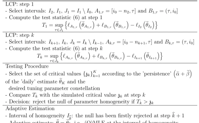
. This adaptive estimate at fixed observation i₀ is then finally used for short-term prediction of the considered (volume or order flow) time series. A short summary of the local adaptive multiplicative error modelling framework, i.e., the local change point (LCP) detection test and the adaptive estimation at fixed observation i0, is for convenience provided in Table 1.

LCP: step 1

- Select intervals: I₂, I₁, J₁ =I₁\I₀, A_1,τ = [i₀−n₂, τ] and B_1,τ = (τ, i₀] - Compute the test statistic (6) at step 1

T1 = sup

τ∈J₁

n`A1,τ

θeA1,τ

+`B1,τ

θeB1,τ

−`I2

θeI2

o

LCP: step k

- Select intervals: I_k+1,I_k, J_k =I_k\Ik−1,A_k,τ = [i₀−n_k+1, τ] and B_k,τ = (τ, i₀] - Compute the test statistic (6) at step k

T_k = sup

τ∈J_k

n`<sub>Ak,τ</sub> θ<sup>e</sup><sub>Ak,τ</sub>+`_Bk,τθ^e_Bk,τ−`_Ik+1θ^e_Ik+1^o Testing Procedure

- Select the set of critical values {z_k}^K_k=1 according to the ’persistence’ α_e +β^e of the ’daily’ estimate θ^e_K and the

desired tuning parameter constellation

- Compare T_k with the simulated critical value z_k at step k - Decision: reject the null of parameter homogeneity if T_k >z_k Adaptive Estimation

- Interval of homogeneity I

b^k: the null has been firstly rejected at step k^b+ 1 - Adaptive estimate: θ^b=^fθ

b^k

, i.e., (Q)MLE at the interval of homogeneity

Table 1: Summary of the local change point (LCP) detection test and the adaptive estimation at fixed observation i₀. Here τ denotes the unknown change point and n_k represents the length of the interval I_k. Source: Härdle et al. (2014). The table has been slightly adjusted to our exposition.

4 Order Flow Dynamics

Empirical results related to the adaptive modelling and forecasting of order flow series are discussed in this section. The presented local adaptive methodology is now applied to the analysed time series, namely, the (seasonally adjusted) buyer-initiated volume, the (seasonally adjusted) seller-initiated volume, the order flow and the relative order flow series. The order flow is given as the difference between the buyer and seller-initated volume, whereas the relative order flow is calculated as a ratio between the buyer-initiated volume and the total volume.

4.1 Adaptive Estimation

The simulation of the critical values is for the analysed time series based on the quartiles of the corresponding estimated daily MEM parameters. For the period from 14 August 2012 to 24 May 2013, Table 2 illustrates the resulting quartiles. One observes higher (daily) persistenceαe +β^e for the volume series, as compared to the order flow dynamics.

This nine cases build our starting point while simulating the critical values for the local change point detection test. Since the values for the volume series exhibit similar results, it is quite convenient to use the average parameter constellations for fixed persistence level in the simulation.

By employing the local adaptive multiplicative error model testing procedure, one selects (nested with right-end fixed) data intervals. A scheme with K + 1 = 15 intervals has been employed. The lengths of the selected intervals are therefore:

{15,19,24,30,38,48,60,75,94,118,148,185,231,289,360}.

For convenience we use 360 observations (i.e., one trading day) in the last selected interval and employ the EACD(1,1) model.

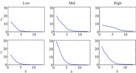
Simulated critical values for parameters of the volume and order flow series are displayed in Figure 3. As already pointed out, we focus on the average values between the buyer-

Model Buyer-initiated Seller-initiated Order Flow

Low Mid High Low Mid High Low Mid High

ωe 0.10 0.22 0.46 0.10 0.21 0.38 0.17 0.23 0.32 αe 0.11 0.16 0.19 0.12 0.15 0.17 0.12 0.18 0.22 βe 0.45 0.63 0.73 0.52 0.66 0.74 0.24 0.36 0.45 αe+β^e 0.56 0.79 0.92 0.64 0.81 0.91 0.36 0.54 0.67

Table 2: Quartiles of estimated MEM parameters based on an estimation window covering one day, i.e., 360 observations, for the buyer and seller initiated volume series, as well as for the order flow series from 14 August 2012 to 24 May 2013 (187 trading days) using the EACD model specification. The order flow series represents the ratio of the buyer initiated volume to the total volume (buyer and seller initiated volume). We label the first quartile as ’low’, the second quartile as ’mid’ and the third quartile as ’high’.

initiated and the seller-initiated series while simulating the critical values for the volume series. The resulting critical value curves do not change significantly between different persistence levels. Already after few steps the critical value curves exhibit stable patterns.

The presence of outliers significantly changes the length of the selected intervals of homo- geneity, see Härdle et al. (2014). In the testing procedure we therefore carefully analysed the effect of the largest observed three values (i.e., data points) within each interval. This selection indeed provides identical evidence (for brevity these results are not shown here).

In order to account for potential sensitivity of the simulation results, we adopt a data driven approach to select critical value curves in the testing procedure. At each minute of the testing procedure we thus select the critical values that are closest to the reported daily persistence level in Table 2. For example, the estimated parameter vector over the past 360 observations for the buyer-initiated volume on 30 April 2013 at 14:00 is (0.07,0.22,0.69)^>. Since the persistence level equalsαe+β^e= 0.22 + 0.69 = 0.91, we select the critical values based on the high persistence level.

It is a reasonable practice to use up to 2 hours of observed data in the modelling of trading volume and (relative) order flow time series at a given trading minute, see, e.g., Figure 4. By selecting the interval lengths based on the interval of homogeneity, one strikes a balance between parameter variability and the modelling bias. As supported by current

0 5 10 0

10 20 30 zk

Low

0 5 10

0 10 20

30 Mid

0 5 10

0 10 20

30 High

0 5 10

0 10 20 30

k zk

0 5 10

0 10 20 30

k

0 5 10

0 10 20 30

k

Figure 3: Simulated critical values of an EACD(1,1) model and chosen parameter con- stellations according to Table 2. Volume series upper panel, order flow lower panel. For the volume series, the average values between the buyer-initiated and seller-initiated se- ries are selected. The curves are associated with the low (blue), mid (green) and high (red) persistence levels (αe+β).^e

Sep 2012 Nov 2012 Jan 2013 Mar 2013 May 2013

0 60

120 Buyer−initiated volume

Sep 2012 Nov 2012 Jan 2013 Mar 2013 May 2013

0 60

120 Seller−initiated volume

Sep 2012 Nov 2012 Jan 2013 Mar 2013 May 2013

0 60

120 Relative order flow

Figure 4: Estimated length of intervals of homogeneity (in minutes) for buyer-initiated, seller-initiated and the order flow series expressed as the ratio between the buyer-initiated volume and the total volume, buyer-initiated and the seller-initiated volume series

Sep Jan May 30

32 34

Length

Buyer−initiated

Sep Jan May

30 32

34 Seller−initiated

Sep Jan May

46 48

50 Relative order flow

Sep Jan May

0.3 0.4 0.5

Persistence

Trading Day 0.3Sep Jan May

0.4 0.5

Trading Day

Sep Jan May

0.3 0.4 0.5

Trading Day

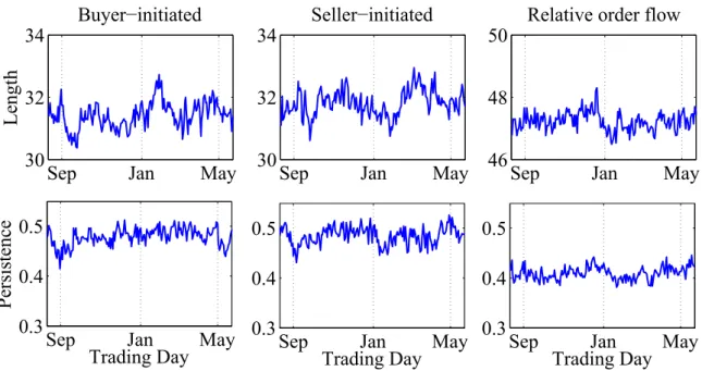
Figure 5: Average estimated daily length of intervals of homogeneity (in minutes) and average daily persistence for buyer-initiated volume, seller-initiated volume and relative order flow series from 14 August 2012 to 24 May 2013 (186 trading days).

9 11 13 15

0 30 60

Length

Buyer−initiated

9 11 13 15

0 30 60

Seller−initiated

9 11 13 15

0 30 60

Relative order flow

9 11 13 15

0.2 0.4 0.6

Persistence

Trading Hour 0.29 11 13 15

0.4 0.6

Trading Hour

9 11 13 15

0.2 0.4 0.6

Trading Hour

Figure 6: Average estimated length of intervals of homogeneity (in minutes) and per- sistence for buyer-initiated volume, seller-initiated volume and relative order flow series over a course of a typical trading day.

literature on adaptive high-frequency forecasting, this leads to significantly better results as compared to the ad hoc selection of estimation windows.

Finally, the average values of the obtained resulting intervals of homogeneity are pro- vided in Figures 5, across trading days, and 6, over the course of a typical trading day.

Apparently the length of the selected average daily intervals are relatively shorter at the end of the respective futures series; recall that the contract months follow a quarterly cycle: Mar (H), Jun (M), Sep (U), and Dec (Z). Even after accounting for intraday- periodicity, we observe a slight increase in the length of the selected intervals during the day. This observation is most likely caused by the overnight effect, since in modelling at the beginning of a trading day we use previous day’s data.

4.2 Forecasting Order Flow Series

Based on the adaptive modelling results we proceed with the short-term adaptive fore- casting as this represents an important step in intra-day trading. Our forecasting period covers the period from 14 August 2012 to 23 May 2013 (e.g., 186 trading days). The recursively computed forecasts are updated at each minute, and we consider the horizons h= 1, . . . ,5 min. The selection of 5 minutes is motivated by significant outperformance of the local parametric approach relative to the benchmark with an ad hoc selected in- terval length, see Härdle et al. (2014). The forecasts of the seasonally adjusted series are multiplied by the seasonality component associated with the previous 30 days in order to avoid forward looking biases.

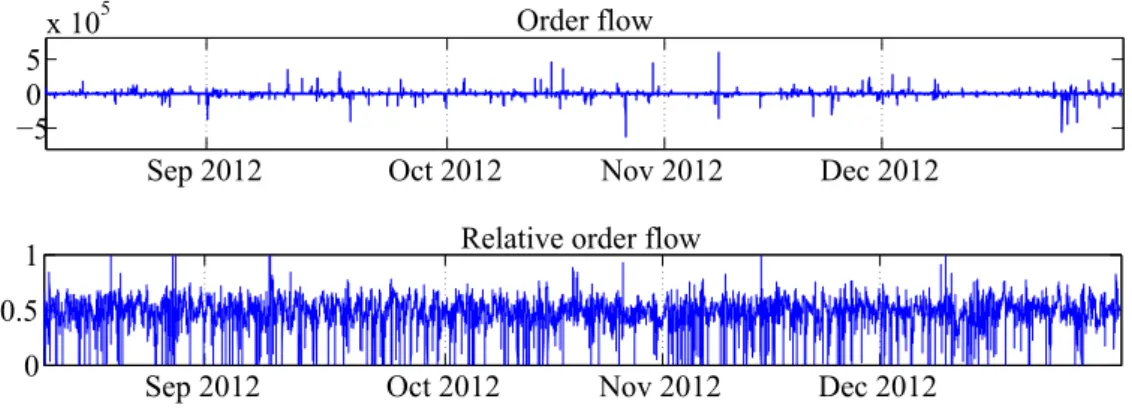
Figure 7 plots the predicted order flow and relative order flow series in 2012, i.e., during the period from 14 August to 28 December 2012 (94 trading days), whereas Figure 8 displays the results during the remaining 92 trading days (in 2013), i.e., from 4 January to 23 May 2013. The plots thus display the predictions of the (relative) order flow series over the forecasting horizon (here set to 5 minutes) at each trading minute.

Our out-of-sample analysis shows that the predictions exhibit scale comparable results

Sep 2012 Oct 2012 Nov 2012 Dec 2012

−505x 10⁵ Order flow

Sep 2012 Oct 2012 Nov 2012 Dec 2012 0

0.5

1 Relative order flow

Figure 7: Predicted (relative) order flow at each minute during the period from 14 August to 28 December 2012 (94 trading days). The forecasting horizon is set to 5 minutes.

Jan 2013 Feb 2013 Mar 2013 Apr 2013 May 2013

−505x 10⁵ Order flow

Jan 20130 Feb 2013 Mar 2013 Apr 2013 May 2013 0.5

1 Relative order flow

Figure 8: Predicted (relative) order flow at each minute during the period from 4 January and 23 May 2013 (92 trading days). The forecasting horizon is set to 5 minutes.

during both trading periods. There are, however, far less atypically large (by magnitude) observations while analysing the order flow series during the second period (i.e., in the first half of 2013). The relative order flow series exhibits strikingly a relatively low number of very low volume predictions during the second (evaluation) period. This is here attributed to the relatively low persistence levels.

The appearance of outliers has a significant impact on the length of the selected intervals of homogeneity, see Härdle et al. (2014). This effect is here again confirmed by comparing the forecasting results displayed in Figures 7 and 8 with the series of selected intervals of homogeneity, see Figure 5. In periods with relatively many outliers the selected interval of homogeneity shrinks and vice versa. In the relatively calm periods it is consequently safe to assume relatively longerintervals of homogeneity as opposed to periods with more trading activity concentrated over relatively short time period.

5 Intra-Day Trading

The local adaptive multiplicative error model exhibits outstanding short term out-of- sample forecasting performance, see Härdle et al. (2014). This section addresses the research question to which extend this framework improves intra-day trading activities.

Our goal here is to analyse the performance of several trading strategies, as well as to achieve statistical arbitrage opportunities. In order to avoid forward looking biases, the sample period is split into two non-overlapping phases, namely, the calibration period and the evaluation period. During the former phase we analyse the results of the proposed (intra-day) trading strategies, whereas during the later period our results are evaluated.

5.1 Trading Strategies and the Calibration Phase

In market microstructure, order flow essentially suggests the direction of the market.

When there are more buy market orders than sell market orders, then the market direction

would be typically up. Accordingly, more sell orders would lead to a price decrease.

Recall, we measure the order flow as the difference between the aggregate sizes of buyer- initiated and seller-initiated trades. The relative order flow is accordingly given by the ratio of the buyer-initiated volume to the total volume (sum of the buyer-initiated and the seller-initiated volume). This two series are observed and predicted at every minute in our sample.

The profitability of the local adaptive multiplicative error models in futures trading is here assessed through the profit or loss resulting from ’trading’ one futures contract over the forecasted period. Our study starts with a new transaction at the end of the current minute and the offset transaction is made at the end of the forecasted period of 5 minutes. For example, let us suppose that the trader starts the trading at 09:02. At the beginning of 09:02 the volume and (relative) order flow series before (and including) 09:01 is observed. Using the methodology presented above, the (relative) order flow series for minutes 09:02,..., 09:06 are predicted. Based on the the resulting forecasts, at end of 09:02 the trader enters a position which is closed at end of 09:06. This process continues at 09:03 and goes until 14:54.

Motivated by the common suggestion that positive (negative) order flow suggests the mar- ket to likely go up (down), we distinguish between the following three trading strategies:

- Strategy (i) ’Buy if positive and sell if negative’ - if the predicted order flow ex- ceeds zero (or a given threshold) then the futures are ’bought’ now and ’sold’ after 5 minutes and if the predictions do not exceed the threshold then the opposite posi- tions are entered. Concerning the relative order flow series, the futures are ’bought’

(’sold’) at the current minute if the predicted relative order flow exceeds 0.50 or a given threshold and ’sold’ (’bought’) at the end of the forecasting period of 5 minutes. Effectively we select two threshold levels; either the threshold equals zero or it is represented by the 95th percentile of the corresponding time series.

- Strategy (ii)’Buy if positive’ - this strategy may be interesting to buyers that expect the Nikkei Stock Average (Nikkei 225) index to rise. The contracts are ’bought’ only

Sep Oct Nov Dec

−500 0 500

Strategy (i)

Sep Oct Nov Dec

−500 0 500

Strategy (ii)

Sep Oct Nov Dec

−500 0 500

Strategy (iii)

Sep Oct Nov Dec

−500 0 500

Sep Oct Nov Dec

−500 0 500

Sep Oct Nov Dec

−500 0 500

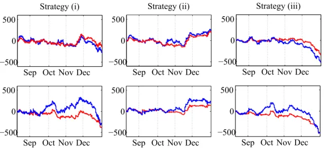
Figure 9: Cumulative profit in thousands Uper one contract during the calibration phase between 14 August (09:01) and 28 December 2012 (15:00), 94 trading days. The equity curves correspond to order flow predictions (upper panel) and to the relative order flow predictions (lower panel). The strategies with zero threshold are shown with blue lines and strategies with non-zero threshold are shown with red lines. The forecasting horizon is set to 5 minutes.

if the predicted (relative) order flow series exceeds some threshold. The threshold level equals zero or equals to the 95th percentile of the series of predicted (relative) order flow series.

- Strategy (iii) ’Sell if negative’ - as opposed to Strategy (ii), this strategy may be interesting to sellers that expect the Nikkei Stock Average (Nikkei 225) index to fall. The contracts are ’sold’ only if the predicted (relative) order flow series does not exceeds some threshold. Again, either the threshold equals zero or it equals to the 95th percentile of the predicted (relative) order flow time series.

During the calibration period from 14 August to 31 December 2012 one observes that the strategy (ii) can been considered best, see, e.g., Figure 9, as it leads to positive results though the calibration phase. Interestingly, the results based on order flow series are relatively insensitive to the threshold selection. Note, however, that the threshold may improve the performance of strategy (iii). Performance of the strategies based on relative order flow predictions reveals that the threshold leads to same final results at the end of

Jan Feb Mar Apr May

−1000 0 1000

Strategy (i)

Jan Feb Mar Apr May

−1000 0 1000

Strategy (ii)

Jan Feb Mar Apr May

−1000 0 1000

Strategy (iii)

Jan Feb Mar Apr May

−1000 0 1000

Jan Feb Mar Apr May

−1000 0 1000

Jan Feb Mar Apr May

−1000 0 1000

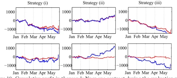
Figure 10: Cumulative profit in thousandsUper one contract during the evaluation phase between 4 January (09:01) and 23 May 2013 (15:00), 92 trading days. The equity curves correspond to order flow predictions (upper panel) and to the relative order flow predic- tions (lower panel). The strategies with zero threshold are shown with blue lines and strategies with non-zero threshold are shown with red lines. The forecasting horizon is set to 5 minutes.

the calibration, although the dynamics suggest that a zero threshold to be better. The performance of the ’buy if positive and sell if negative’ strategy (i) is to a large extend influenced by the (negative) results of ’buy if negative’ trading activity.

5.2 Trading Profit Evaluation

The previously discussed trading strategies are now applied to data following the calibra- tion phase, i.e., here the sample period from 4 January to 23 May 2013 covers 92 trading days. The results are presented in Figure 10.

Clearly the proposed trading strategy (ii) ’Buy if positive’ outperforms the other strate- gies by a large margin. The cumulated profits are scale comparable to the results obtained during the calibration phase. Based on the resulting profits, in most cases the threshold values lead to slight improvements of the strategies. As with the calibration period, one should be careful and not include the threshold component while employing the winning strategy.

There are no visible (quarterly) effects due to the different futures series, although this has been indicated by the analysis of the selectedintervals of homogeneity. This confirms that adaptive selected methods indeed play a crucial role in order flow dynamics modelling.

It would be therefore inappropriate to use an ad hoc selected window length, see also Härdle et al. (2014).

6 Conclusions

Adaptive order flow modelling is suitable for understanding of the imbalances in trades initiated by market orders at transaction level. By employing the so-calledLocal adaptive multiplicative error models by Härdle et al. (2014), the trading volume and order flow dynamics of the analysed futures series has been captured successfully. Our flexible adaptive approach yields potentially varying lengths of the ’optimal’ estimation windows.

Local windows of approximately 1-2 hours are reasonable to capture the dynamics of the analysed order flow series. Interestingly, we found a slightly pronounced quarterly pattern in the selected length of the so-calledinterval of homogeneity.

Order flow dynamics provides valuable information for inferring the direction of price moves. In forecasting and intra-day trading, the proposed approach exhibits remarkable results. The best statistical outperformance relative to a benchmark with ad hoc selected intervals is achieved at forecasting horizons up to 3-5 minutes, see Härdle et al. (2014).

For this reason we used 5 minutes for the forecasting horizon in the intra-day trading example. The most profitable in-sample based strategy (ii) ’Buy if positive’ (where the contracts are ’bought’ only if the predicted (relative) order flow series exceeds zero) leads also to best out-of-sample results.

References

Cairney, T. and Swisher, J. (2004). The role of the options market in the dissemination of private information, Journal of Business Finance and Accounting31: 1015–1041.

Chan, K. and Fong, W.-M. (2000). Trade size, order imbalance and the volatility-volume relation, Journal of Financial Economics57: 247–273.

Chen, Y., Härdle, W. and Pigorsch, U. (2010). Localized Realized Volatility, Journal of the American Statistical Association105(492): 1376–1393.

Chordia, T., Roll, R. and Subrahmanyam, A. (2002). Order imbalance, liquidity, and market returns, Journal of Financial Economics65: 111–130.

Chordia, T., Subrahmanyam, A. and Anshuman, V. R. (2001). Trading activity and expected stock returns, Journal of Financial Economics59: 3–32.

Čížek, P., Härdle, W. K. and Spokoiny, V. (2009). Adaptive pointwise estimation in time- inhomogeneous conditional heteroscedasticity models, Econometrics Journal 12: 248–

271.

Engle, R. F. (2002). New Frontiers for ARCH Models, Journal of Applied Econometrics 17: 425–446.

Engle, R. F. and Rangel, J. G. (2008). The Spline-GARCH Model for Low-Frequency Volatility and Its Global Macroeconomic Causes,Review of Financial Studies21: 1187–

1222.

Engle, R. F. and Russell, J. R. (1998). Autoregressive Conditional Duration: A New Model for Irregularly Spaced Transaction Data,Econometrica 66(5): 1127–1162.

Gallant, A. R. (1981). On the bias of flexible functional forms and an essentially unbiased form, Journal of Econometrics 15: 211–245.

Härdle, W. K., Hautsch, N. and Mihoci, A. (2014). Local Adaptive Multiplicative Error Models for High-Frequency Forecasts, Journal of Applied Econometrics, DOI:

10.1002/jae.2376.

Hautsch, N. (2012). Econometrics of Financial High-Frequency Data, Springer, Berlin.

Jones, C. M., Kaul, G. and Lipson, M. L. (1994). Transactions, volume, and volatility, Review of Financial Studies 7: 631–651.

Mercurio, D. and Spokoiny, V. (2004). Statistical inference for time-inhomogeneous volatility models, The Annals of Statistics32(2): 577–602.

Spokoiny, V. (1998). Estimation of a function with discontinuities via local polynomial fit with an adaptive window choice, The Annals of Statistics26(4): 1356–1378.

SFB 649 Discussion Paper Series 2014

For a complete list of Discussion Papers published by the SFB 649, please visit http://sfb649.wiwi.hu-berlin.de.

001 "Principal Component Analysis in an Asymmetric Norm" by Ngoc Mai Tran, Maria Osipenko and Wolfgang Karl Härdle, January 2014.

002 "A Simultaneous Confidence Corridor for Varying Coefficient Regression with Sparse Functional Data" by Lijie Gu, Li Wang, Wolfgang Karl Härdle and Lijian Yang, January 2014.

003 "An Extended Single Index Model with Missing Response at Random" by Qihua Wang, Tao Zhang, Wolfgang Karl Härdle, January 2014.

004 "Structural Vector Autoregressive Analysis in a Data Rich Environment:

A Survey" by Helmut Lütkepohl, January 2014.

005 "Functional stable limit theorems for efficient spectral covolatility estimators" by Randolf Altmeyer and Markus Bibinger, January 2014.

006 "A consistent two-factor model for pricing temperature derivatives" by Andreas Groll, Brenda López-Cabrera and Thilo Meyer-Brandis, January 2014.

007 "Confidence Bands for Impulse Responses: Bonferroni versus Wald" by Helmut Lütkepohl, Anna Staszewska-Bystrova and Peter Winker, January 2014.

008 "Simultaneous Confidence Corridors and Variable Selection for Generalized Additive Models" by Shuzhuan Zheng, Rong Liu, Lijian Yang and Wolfgang Karl Härdle, January 2014.

009 "Structural Vector Autoregressions: Checking Identifying Long-run Restrictions via Heteroskedasticity" by Helmut Lütkepohl and Anton Velinov, January 2014.

010 "Efficient Iterative Maximum Likelihood Estimation of High- Parameterized Time Series Models" by Nikolaus Hautsch, Ostap Okhrin and Alexander Ristig, January 2014.

011 "Fiscal Devaluation in a Monetary Union" by Philipp Engler, Giovanni Ganelli, Juha Tervala and Simon Voigts, January 2014.

012 "Nonparametric Estimates for Conditional Quantiles of Time Series" by Jürgen Franke, Peter Mwita and Weining Wang, January 2014.

013 "Product Market Deregulation and Employment Outcomes: Evidence from the German Retail Sector" by Charlotte Senftleben-König, January 2014.

014 "Estimation procedures for exchangeable Marshall copulas with hydrological application" by Fabrizio Durante and Ostap Okhrin, January 2014.

015 "Ladislaus von Bortkiewicz - statistician, economist, and a European intellectual" by Wolfgang Karl Härdle and Annette B. Vogt, February 2014.

016 "An Application of Principal Component Analysis on Multivariate Time- Stationary Spatio-Temporal Data" by Stephan Stahlschmidt, Wolfgang Karl Härdle and Helmut Thome, February 2014.

017 "The composition of government spending and the multiplier at the Zero Lower Bound" by Julien Albertini, Arthur Poirier and Jordan Roulleau- Pasdeloup, February 2014.

018 "Interacting Product and Labor Market Regulation and the Impact of Immigration on Native Wages" by Susanne Prantl and Alexandra Spitz- Oener, February 2014.

SFB 649, Spandauer Straße 1, D-10178 Berlin http://sfb649.wiwi.hu-berlin.de

This research was supported by the Deutsche

Forschungsgemeinschaft through the SFB 649 "Economic Risk".

SFB 649, Spandauer Straße 1, D-10178 Berlin http://sfb649.wiwi.hu-berlin.de

This research was supported by the Deutsche

Forschungsgemeinschaft through the SFB 649 "Economic Risk".

SFB 649, Spandauer Straße 1, D-10178 Berlin http://sfb649.wiwi.hu-berlin.de

This research was supported by the Deutsche

Forschungsgemeinschaft through the SFB 649 "Economic Risk".

SFB 649 Discussion Paper Series 2014

For a complete list of Discussion Papers published by the SFB 649, please visit http://sfb649.wiwi.hu-berlin.de.

019 "Unemployment benefits extensions at the zero lower bound on nominal interest rate" by Julien Albertini and Arthur Poirier, February 2014.

020 "Modelling spatio-temporal variability of temperature" by Xiaofeng Cao, Ostap Okhrin, Martin Odening and Matthias Ritter, February 2014.

021 "Do Maternal Health Problems Influence Child's Worrying Status?

Evidence from British Cohort Study" by Xianhua Dai, Wolfgang Karl Härdle and Keming Yu, February 2014.

022 "Nonparametric Test for a Constant Beta over a Fixed Time Interval" by Markus Reiß, Viktor Todorov and George Tauchen, February 2014.

023 "Inflation Expectations Spillovers between the United States and Euro Area" by Aleksei Netšunajev and Lars Winkelmann, March 2014.

024 "Peer Effects and Students’ Self-Control" by Berno Buechel, Lydia Mechtenberg and Julia Petersen, April 2014.

025 "Is there a demand for multi-year crop insurance?" by Maria Osipenko, Zhiwei Shen and Martin Odening, April 2014.

026 "Credit Risk Calibration based on CDS Spreads" by Shih-Kang Chao, Wolfgang Karl Härdle and Hien Pham-Thu, May 2014.

027 "Stale Forward Guidance" by Gunda-Alexandra Detmers and Dieter Nautz, May 2014.

028 "Confidence Corridors for Multivariate Generalized Quantile Regression"

by Shih-Kang Chao, Katharina Proksch, Holger Dette and Wolfgang Härdle, May 2014.

029 "Information Risk, Market Stress and Institutional Herding in Financial Markets: New Evidence Through the Lens of a Simulated Model" by Christopher Boortz, Stephanie Kremer, Simon Jurkatis and Dieter Nautz, May 2014.

030 "Forecasting Generalized Quantiles of Electricity Demand: A Functional Data Approach" by Brenda López Cabrera and Franziska Schulz, May 2014.

031 "Structural Vector Autoregressions with Smooth Transition in Variances – The Interaction Between U.S. Monetary Policy and the Stock Market" by Helmut Lütkepohl and Aleksei Netsunajev, June 2014.

032 "TEDAS - Tail Event Driven ASset Allocation" by Wolfgang Karl Härdle, Sergey Nasekin, David Lee Kuo Chuen and Phoon Kok Fai, June 2014.

033 "Discount Factor Shocks and Labor Market Dynamics" by Julien Albertini and Arthur Poirier, June 2014.

034 "Risky Linear Approximations" by Alexander Meyer-Gohde, July 2014 035 "Adaptive Order Flow Forecasting with Multiplicative Error Models" by

Wolfgang Karl Härdle, Andrija Mihoci and Christopher Hian-Ann Ting, July 2014