Combustion Simulations in Diesel Engines using Reduced Reaction Mechanisms

using

Reduced Reaction Mechanisms

D I S S E R T A T I O N submitted to the

Combined Faculties for the Natural Sciences and for Mathematics of the Rupertus Carola University of Heidelberg, Germany

for the degree of Doctor of Natural Sciences

presented by

Chrys Correa, M.S. (Chem. Eng.) born in Bombay

Examiners: Prof. Dr. Dr. h.c. J¨urgen Warnatz Prof. Dr. Bernhard Schramm Heidelberg, June 30, 2000

Interdisziplin¨ares Zentrum f¨ur Wissenschaftliches Rechnen Ruprecht - Karls - Universit¨at Heidelberg

2000

submitted to the

Combined Faculties for the Natural Sciences and for Mathematics of the Rupertus Carola University of

Heidelberg, Germany for the degree of Doctor of Natural Sciences

presented by

Chrys Correa, M.S. (Chem. Eng.) born in Bombay

Heidelberg, June 30, 2000

Combustion Simulations in Diesel Engines using

Reduced Reaction Mechanisms

Examiners: Prof. Dr. Dr. h.c. J¨urgen Warnatz Prof. Dr. Bernhard Schramm

The simulation of combustion in internal combustion engines is important in order to make computer-aided design possible, and also to be able to predict pollutant formation and gain a better understanding of the coupling between the various physical and chemical processes. Accurate simulations of Diesel engines require models for the various processes, such as spray dynamics, ignition, chemistry, heat transfer, etc. as well as the interactions between them, such as chemistry-turbulence interactions, etc.

A standard finite-volume CFD (computational fluid dynamics) code, KIVA III, which is capable of simulating two-phase engine flows was used. KIVA solves the three- dimensional Navier-Stokes equations, which are Favre-averaged, with a k-turbulence model. The spray dynamics are handled using a discrete droplet model (DDM) along with sub-models for collision, breakup, evaporation, etc. Three areas were identified, where KIVA sub-models either do not exist, or are insufficiently detailed for pollutant formation prediction: ignition, chemistry and radiation heat transfer. New models were developed and implemented for these three processes, which contain more physics and chemistry than the previous models, but which are computationally within limits for simulating a three-dimensional engine.

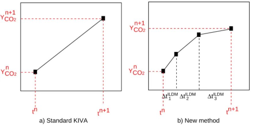
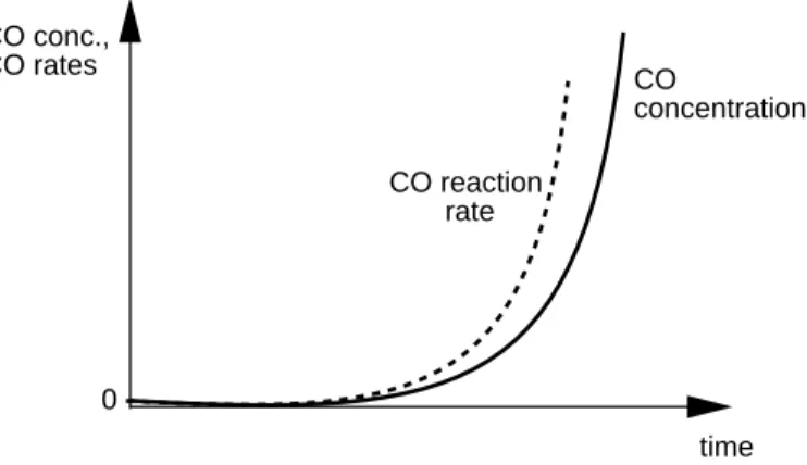
Ignition modeling in Diesel engines is very important to identify the ignition delay and the location of auto-ignition. As soon as the fuel is injected into the engine, low-temperature reactions occur leading to the formation of a radical pool. The con- centration of this radical pool then increases during the ignition delay period due to chain reactions, eventually leading to ignition. Ignition chemistry can be described by means of a detailed chemical mechanism, which however cannot be used in a practical engine simulation due to the large number of species involved. In this thesis, igni- tion was tracked by means of a representative species (here CO), whose concentration remains almost zero during the ignition period and which shows a sharp increase at ignition. The reaction rate of CO was obtained from the detailed mechanism as a func- tion of a few variables. In order to use this approach in turbulent flows, the reaction rate was integrated over a presumed probability density function (pdf) to account for the interactions between chemistry and turbulence.

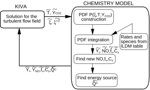
Chemistry models used in Diesel engines should be capable of predicting intermediate and minor species in order to accurately capture the flame propagation and predict pollutant formation. The intrinsic low-dimensional manifold (ILDM) method was used in this thesis. It is an automatic reduction of a detailed chemical mechanism based on a local time scale analysis. Here, chemical processes which are fast in comparison to the turbulent mixing time scale are assumed to be in dynamic equilibrium. This allows the chemistry to be expressed only in terms of a few progress variables. Here, with n-heptane as a model diesel fuel, a one-dimensional ILDM with the CO2 concentration as the progress variable. This chemistry model was also combined with a presumed probability density function (pdf) method in order to enable its use in turbulent flames.

NOx and soot were identified as the main pollutants and were predicted using a Zel- dovich model and a phenomenological two-equation model, respectively with the NO

concentration is high. The six-dimensional radiative transfer equation (RTE) needs to be solved for the radiative intensity along with models describing the variation of the radiative properties (e.g., absorption coefficients) with wavelength. The radiative properties of the gases (CO2 and H2O) were described with a weighted sum of grey gases model (WSGGM), where the total emissivity of a non-grey gas is represented by the weighted sum of the emissivities of a small number of grey gases. The radiative properties of soot were described by a grey model. The RTE was solved using the discrete ordinates method (DOM), which involves solving the RTE in discrete directions to describe the angular dependence of the intensity. Turbulence-radiation interactions were described using a presumed pdf.

The ignition and chemistry models were implemented in KIVA and used to simulate the combustion in a Caterpillar Diesel engine, for which experimental data were avail- able. Simulations were carried out for several injection timings. In all simulations, ignition was observed to occur at the edge of the spray, in the lean-to-stoichiometric region where the temperatures are higher. Thermal NO formation was seen in the stoichiometric region at high temperatures, while soot formation was seen in the richer region where the temperatures are low. Simulated pressure curves were compared to experimental data and showed good agreement. The mean NO at the end of the cycle was compared to experimental values and also showed reasonable agreement (a max- imum deviation of about 20% was observed). The mean soot at the end of the cycle was strongly under-predicted due to the inability to identify the one-dimensional man- ifold in the rich region where the formation of soot precursors is dominant. The DOM radiation model was tested in a furnace with a known temperature and absorption coefficient distribution, and the wall fluxes were compared to analytical data. It was not used in the engine due to low quantities of soot predicted. Instead, an optically thin model along with the WSGGM was used in the engine and the radiative losses were seen to be negligible.

1 Introduction 1 2 Equations for turbulent reactive flows with sprays 5

2.1 Gas-phase equations . . . 5

2.1.1 Species mass balance . . . 5

2.1.2 Total mass balance . . . 5

2.1.3 Momentum balance . . . 6

2.1.4 Energy balance . . . 6

2.1.5 State relations . . . 7

2.2 Averaging of the gas phase equations . . . 7

2.2.1 Favre-averaged equations . . . 9

2.3 Turbulence models . . . 10

2.3.1 The k- turbulence model . . . 11

2.4 Spray modeling . . . 12

2.4.1 Spray equations . . . 13

2.4.2 Collision . . . 14

2.4.3 Breakup . . . 15

2.4.4 Evaporation . . . 16

2.4.5 Droplet acceleration . . . 18

2.4.6 Gas-spray interaction terms . . . 19

2.5 Chemistry modeling . . . 19

2.5.1 Detailed reaction mechanisms . . . 19

2.5.2 Global reaction mechanisms . . . 20

2.5.3 Equilibrium chemistry . . . 21

2.6 Chemistry-turbulence interactions . . . 22

2.6.1 Mean reaction rates using mean values . . . 22

2.6.2 Mean reaction rates using pdfs . . . 23

3 Models for ignition, chemistry and radiation 25 3.1 Ignition . . . 25

3.1.1 Ignition chemistry . . . 25

3.1.2 Ignition in turbulent flames . . . 27

3.2.1 Principles behind ILDM . . . 31

3.2.2 Mathematical treatment of ILDM . . . 32

3.2.3 Use of ILDM and problems . . . 33

3.2.4 ILDM with pdfs . . . 38

3.3 Pollutant formation . . . 41

3.3.1 NOx formation . . . 41

3.3.2 Soot formation . . . 42

3.4 Radiation heat transfer . . . 47

3.4.1 Radiative properties . . . 49

3.4.2 Solution methods for the RTE . . . 54

3.4.3 Turbulence-radiation interactions . . . 59

4 Numerical simulation with KIVA 60 4.1 Temporal differencing . . . 60

4.2 Spatial differencing . . . 62

4.3 Coupling between KIVA and new models . . . 63

5 Results in a Diesel engine 67 5.1 Engine specifications . . . 67

5.2 Cold flow . . . 69

5.3 Ignition results . . . 71

5.4 Flame propagation . . . 73

5.5 Pollutant formation . . . 74

5.6 Comparison with experiments . . . 77

5.7 Radiation results . . . 80

5.7.1 Radiation in a simplified geometry . . . 80

5.7.2 Radiation in the engine . . . 85

6 Conclusions and recommendations 87

1 Introduction

Combustion processes are very important in our day-to-day lives and also in industrial processes. About 90% of our energy requirements (e.g., in electrical power generation, heating, chemical industry, etc.) is provided by combustion. In spite of this impor- tance, the fundamental processes occurring in combustion and their interactions with each other are not completely understood. Commonly used fuels in the industry are hydrocarbons and coal. These fuels are not available in unlimited amounts, hence there exists a need to run combustion processes more economically. Additionally, there exists the need to optimize either the operating or the geometrical parameters of the process in order to minimize environmental risks, e.g., the emission of unburnt hydrocarbons which are carcinogenic.

Since the experimental design of complex practical combustion devices is difficult and expensive, numerical simulations provide an attractive alternative for practical design.

Mathematical modeling of reactive flows has gained increasing importance in the last decades. A large variety of models describing the several processes occurring in com- bustion, e.g., chemistry, turbulence, etc. and a variety of numerical tools required to solve the underlying equation systems have been developed. The progress of computer technology has also made it possible to simulate these practical devices. Detailed mod- els for physical processes, such as detailed chemical mechanisms or detailed transport, are possible either in laminar flames [1–3] or in turbulent flames with simple geome- tries [4]. However, in practical three-dimensional complex geometries, the use of very simplified models in order to keep the computational requirements affordable is com- mon. These models usually represent simplified versions of the real physical processes, and hence their use requires the specification of several parameters. These parameters usually need to be adjusted for different applications, making the whole process empir- ical. The aim of this thesis is to develop and use models for physical processes which are more detailed and have more physics than commonly used models, but at the same time are computationally feasible for use in practical geometries.

Several practical flames are diffusion flames, i.e., the fuel and the oxidizer enter the combustion chamber separately. Liquid fuels are also common in internal combustion engines, aircraft motors, etc. In order to maximize the surface area per unit mass of the fuel, and thus increase the reaction rates, the liquid fuel is often injected under high pressures. Thus, combustion chambers where liquid fuel is directly injected into the chamber under high pressure are relatively common. These diffusion flames need to be modeled accurately in order to enable the use of the simulation results in practice.

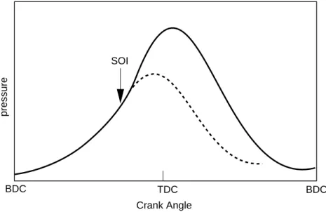
Compression ignition engines are used in a variety of applications - automobile, truck, locomotive, marine, power generation, etc. Here, air alone is inducted into the cylinder, and load control is achieved by varying the amount of fuel injected. The operation of a typical compression ignition engine is illustrated in Figure 1.1. The compression ratio of Diesels is much higher than typical spark ignition engines, and is in the range of 12 to 24. Air at close to atmospheric pressure is inducted at bottom-dead-center (BDC) where the piston is in its lowest position, and compressed to a pressure of about 4

BDC TDC BDC SOI

pressure

Crank Angle

Figure 1.1: Cylinder pressure versus crank angle during compression, combustion and expansion in a typical Diesel cycle (solid line: firing cycle, dashed line: motored cycle)

MPa and temperature of about 800 K during the compression stroke. At about 20^◦ before top-dead-center (TDC), where the piston is in its highest position, fuel injection commences (start of injection, SOI). The air temperature and pressure are above the fuels ignition point, and after a short delay period, spontaneous ignition of the mixture occurs, and the cylinder pressure (solid line in Figure 1.1) rises beyond the non-firing engine level (dashed line in Figure 1.1). The cylinder pressure then decreases due to expansion.

Internal combustion engines are generally more complex to model than other combus- tion chambers due to the following reasons:

• While most combustion processes occur at atmospheric pressure, very high pres- sures are present in engines.

• The presence of two phases, the liquid fuel phase and the gaseous phase, and the important interactions between them requires good models for both phases.

• Most flames do not involve ignition processes which are difficult to model.

• Most combustion chambers have no moving parts, unlike internal combustion engines, where the piston movement needs moving grids.

Most practical flames are turbulent due to the high velocities and large dimensions involved. Thus, the simulation of a general turbulent flame requires models for the dif- ferent underlying processes involved, i.e., chemistry, turbulence, heat transfer through several modes (e.g. conduction, radiation), mass transfer through several modes (e.g., convection, diffusion), etc. and the complex interactions between the processes. All these processes are highly nonlinear and efficient numerical methods need to be used

in order to solve the underlying equations. Partial differential equations can be for- mulated for the balance of mass, momentum and energy. These form a non-linear, elliptical, coupled system of equations which can be solved with standard methods if all the length and time scales involved are resolved. Turbulent flows contain a large range of length scales, ranging from the largest scale dependent on the geometry of the system (the integral length scale) to the smallest scale (the Kolmogorovlength scale).

Resolving all these scales is possible, at present, only for a few low Reynolds-number systems [5]. However, these equations can be averaged and equations can be solved for averaged quantities.

The spray in the system is modeled by using a discrete particle method [6], where the probability distribution of the location, velocity, size and temperature of the droplets is solved for. This model accounts for the break-up, union and collision of the individual droplets. This phase is coupled with the gas phase through an exchange of mass, energy and momentum.

The prediction of the ignition location and its timing is especially important in Diesel engines as the flame propagation that follows is dependent on it. Auto-ignition results due to several low-temperature chain reactions which lead to the formation of a rad- ical pool. The prediction of this radical pool formation without the use of empirical parameters is only possible with the help of detailed chemical mechanisms. In order to enable the use of such mechanisms in a three-dimensional computational fluid dynam- ics (CFD) program, the reaction rates were tabulated and a representative species was chosen to track the buildup of the radical pool.

Chemistry models in engines are usually simplified, e.g., with global reaction assump- tions or equilibrium assumptions. These are computationally cheap, however they cannot accurately predict pollutant formation [7]. On the other hand, detailed chem- ical mechanisms have been found to show good agreement with experimental data in laminar flames [8]. However, these mechanisms involve many species and reactions and thus their use in three-dimensional turbulent flames is limited. In this thesis, a method called the intrinsic low-dimensional manifold (ILDM) [9,10] was used, which is an automatic reduction of a detailed chemical mechanism based on a local eigenvalue analysis. This method enables the prediction of major species as well as minor radicals using only a few progress variables.

The above mentioned averaging of the balance equations leads to unclosed terms in these equations. One of the most difficult terms to close is the chemical source term in the species equation. This term represents the interaction between chemistry and turbulence and can be closed using statistical methods. The presumed-pdf method [11]

was employed in this work. Here, the shape of the probability density function (pdf) is assumed and the chemical source terms are then integrated over this pdf to give their mean.

A mode of heat transfer often neglected in combustion simulations is radiation. This could have an effect on the quantity of pollutants predicted, as pollutant formation is especially sensitive to the temperature. Radiation is difficult to model due to the six- dimensional integro-differential equation that needs to solved for the radiative intensity

distribution [12]. The discrete ordinates method [13] solves this problem by solving the equation in discrete directions. The radiative properties of the gases and the soot also need to be accurately modeled. Since detailed wavelength-dependent calculations are very expensive, a weighted sum of grey gases model (WSGGM) [14] was used, where the non-grey medium is replaced by a small number of grey media with constant absorption coefficients.

The aim of this thesis is to simulate a turbulent spray diffusion flame with pollutant formation in a realistic Diesel engine. For this, an existing three-dimensional code KIVA-III [6] with existing spray models was used. The above mentioned models were implemented and used to describe the ignition, chemistry, chemistry-turbulence inter- actions and radiation. The resulting code was tested with a direct-injection Diesel engine for five different injection timings. The turbulent flow with compression, fuel injection, spray dynamics, mixing, ignition, flame propagation with pollutant forma- tion and heat transfer, and expansion was simulated and the results were compared with experimental data. On the basis of this comparison, the use of these models and the improvements required can be discussed.

Chapter 2 discusses the basic equations used for turbulent, reactive flows with sprays.

Chapter 3 discusses the new ignition model, the chemistry model, the pdf model and the radiation model used. Chapter 4 discusses in brief the numerical methods used in KIVA and the coupling between the new models in Chapter 3 and the equations in Chapter 2. Chapter 5 presents results from the simulations and compares them with experimental data, and Chapter 6 presents conclusions and recommendations.

2 Equations for turbulent reactive flows with sprays

2.1 Gas-phase equations

The fluid flow in internal combustion engines is unsteady, turbulent and compressible.

These flows can be mathematically described by the Navier- Stokes equations [15]. In these equations, it is assumed that equations of continuum mechanics are valid, which is valid when the smallest turbulent eddy is larger than the mean free length of the molecules [16]. These equations describe the balance of mass, energy, and momentum.

A general balance equation for variable φ contains terms due to convection, diffusion, source terms and unsteady terms, and looks like

∂(ρφ)/∂t

Accumulation

+ div(ρuφ)

Convection

= div(Γφgradφ)

Dif f usion

+ Sφ

Source

, (2.1)

where ρ is the density,u is the velocity vector, Γφ is the diffusion coefficient and Sφ is the source/sink term.

2.1.1 Species mass balance

The species balance equation in terms of the species density ρi is given by

∂ρi

∂t + div(ρiu) = div(ρDgrad(ρi

ρ)) + ˙ρiC+ ˙ρiS , (2.2) where ˙ρiC is the source term due to chemistry (see Section 2.5) and ˙ρiS is the source term due to the spray (see Section 2.4). The spray source term applies only to the fuel (always species number 1 in KIVA). The diffusion coefficient Γφhas the form ρDhere.

It is assumed that all the species have equal diffusivities, given by

D= µ

ρSc , (2.3)

where µis the dynamic viscosity (see Section 2.3) and Sc is the Schmidt number (the dimensionless number describing the relationship between viscosity and diffusivity).

2.1.2 Total mass balance

Adding the species transport equations (Equation (2.2)) for all species, one gets the total mass balance equation. Since mass cannot be produced or destroyed in chemical reactions, the only source term is one due to the addition of the fuel spray:

∂ρ

∂t + div(ρu) = ˙ρ1S . (2.4)

2.1.3 Momentum balance

A balance of momentum mu gives the equation

∂(ρu)

∂t + div(ρuu) = div ¯¯σ−gradp+F^S+ρg , (2.5) where p is the fluid pressure. The viscous stress tensor ¯σ¯ for a Newtonian fluid is

¯¯

σ =µ[gradu+ (gradu)^T]− 2

3µ(divu)¯¯I , (2.6) where the exponent T stands for the transpose and ¯¯I is the identity tensor. F^S is the rate of momentum gain per unit volume due to the spray (see Section 2.4).

2.1.4 Energy balance

The equation for the specific internal energyE, excluding the heats of formation of the species involved, is

∂(ρE)

∂t + div(ρuE) =−pdiv(u)−divJ+ρ+ ˙Q^C+ ˙Q^S . (2.7) The heat flux vectorJis the sum of contributions due to heat conduction and enthalpy diffusion,

J =−KgradT −ρD

i

higrad(ρi/ρ) , (2.8)

where T is the fluid temperature, K is the thermal conductivity and hi is the specific enthalpy of species i. K is calculated from the Prandtl number P r and the specific heat at constant pressure cp using

K = µcp

P r , (2.9)

where the specific heat of the mixture is calculated using

cp(T) =

i

ρi

ρcpi(T) . (2.10)

The specific heats of the species cpi as well as the specific enthalpies hi in Equation (2.8) are obtained from the JANAF tables [17] as functions of temperature. The term ρ represents the energy source due to turbulence, where is the dissipation rate of the turbulent kinetic energy. Two source terms arise in Equation (2.7): ˙Q^C due to the chemistry (see Section 2.5) and ˙Q^S due to the spray (see Section 2.4).

2.1.5 State relations

The state relations are assumed to be of an ideal gas, giving equations for the temper- ature and the pressure as

T = 1 R0

i

Mi[hi(T)− ρi

ρE(T)] , (2.11)

p=R0T

i

ρi

Mi

, (2.12)

where Mi is the molar mass of species i and R0 is the ideal gas constant.

2.2 Averaging of the gas phase equations

The gas phase equations defined in Section 2.1 can be directly solved in a deterministic manner for all the unknowns. In order to do this, all the length and time scales involved need to be resolved. In turbulent flows, a number of length scales exist that characterize different aspects of the flow behavior. The integral length scale represents the largest length scale and is governed by the dimensions of the system (about 0.1 m in an engine). The smallest scales are limited by molecular diffusion and are about 10⁻⁵ m [7] in length. To resolve them, one needs about 10⁴mesh points in each direction, i.e.

about 10¹² points in the three-dimensional engine. The smallest time scales are of the order of 10⁻⁶ s and a complete combustion cycle lasts about 50 ms for a speed of 2000 rpm [18], so that about 50,000 time steps are required. About 5×10⁴ floating-point operations are required at each time step at each mesh point. This means that 2.5×10²¹ operations are needed for the entire problem, which can take 350,000 CPU-years on a computer with 300 MFLOPS.

However, since we are only interested in the mean values and not in the instantaneous fluctuations, an averaging of the equations defined in Section 2.1 can be carried out by

splitting each variable into its mean and its fluctuating component and then averaging.

Thus, statistical methods are used to describe the random flow. Several different types of averaging procedures are possible, e.g., time averaging, where the variable is averaged over a definite time interval,

φ(t) = 1 t−t0

t t₀

φ(t)dt . (2.13)

In engines, the application of these turbulence concepts is complicated by the fact that there are cycle-to-cycle variations in the mean flow at any point in the cycle, as well turbulent fluctuations about that specific cycles mean flow [7]. An approach used in such quasi-periodic flows is ensemble averaging, where the variable is averaged over severalNcyc cycles. This averaging process is performed at several crank angle locations to get the ensemble-averaged variable over the entire cycle,

φN_cyc = 1 Ncyc

N_cyc

n=1

φn . (2.14)

Figure 2.1 shows this approach applied to an engine with small and large cycle-to-cycle variations [7].

Thus, each variable can be split into its mean φ and its fluctuation φ,

φ=φ+φ . (2.15)

The mean of the fluctuations φ disappears using

φ = 0 . (2.16)

The mean of the square of the fluctuations is called the variance and can be calculated by

φ² =φ² −φ² . (2.17)

However, since large density variations are common in combustion processes due to large temperature differences, it is useful to introduce a density-weighted average, called the Favre average ˜φ, in order to avoid terms involving density fluctuations,

φ˜= ρφ

ρ . (2.18)

φ

CA Ensemble average

Instantaneous

a) Low cycle−to−cycle variations

φ

CA Ensemble average

b) Large cycle−to−cycle variations

Instantaneous

Individual cycle mean

Figure 2.1: Ensemble averaging of variable φ as a function of the crank angle for a)Small cycle-to-cycle variations, and b)Large cycle-to-cycle variations[7]

Using Favre averaging, a variable φ can now be split into

φ= ˜φ+φ . (2.19)

2.2.1 Favre-averaged equations

Substitution of equations (2.15) and (2.18) in the gas phase equations results in the Reynolds-averaged Navier Stokes equations (RANS), i.e., the Navier Stokes equations in terms of the Favre-averaged variables [19]:

Species mass balance (using ρi =ρYi):

∂ρY˜i

∂t + div(ρu˜Y˜i) = div(ρDgradYi−ρuY_i) +ρY˙i

C+ρY˙i

S (2.20)

Total mass balance:

∂ρ

∂t + div(ρ˜u) = ˙ρiS (2.21)

Momentum balance:

∂(ρ˜u)

∂t + div(ρ˜u˜u) = div(¯σ¯¯−ρuu)−grad ˜p+F^S+ρg˜ (2.22) Energy balance:

∂(ρE)˜

∂t + div(ρ˜uE) =˜ −p˜div ˜u−div(J+ρuE) +ρ˜+ ˙Q^C+ ˙Q^S (2.23) State relations:

T˜ = 1 R0

i

Mi[hi( ˜T)−ρ_i

ρE( ˜˜ T)] (2.24)

˜

p= ρR0T˜

M , (2.25)

where the fluctuations in the mean molar mass M are neglected.

The above mean equations contain correlation terms in the form ofρuφ which repre- sent the effects of turbulent fluctuations. These new terms generated in the averaging process are not known explicitly as functions of the means, leading to more unknowns than equations (the closure problem in turbulence). These terms need to be modeled using turbulence models (see Section 2.3). The mean sources due to chemistry (ρY˙i

C

and ˙Q^C) are described in Sections 2.5 and 2.6. The mean sources due to the spray ( ˙ρiS, F^S, ˙Q^S) are defined in Section 2.4.

2.3 Turbulence models

In order to solve the closure problem, models which describe ρuφ in terms of the mean variables are needed. The eddy-viscosity concept [20] is the most commonly used basis for turbulence models. Here, ρuφ is interpreted as turbulent transport and is modeled analogous to laminar transport, i.e., by analogy with Fick’s law, it is proportional to the gradient of the mean value of the property, but with a turbulent exchange coefficient. The Reynolds stress terms (ρuu) in Equation (2.22) is thus,

ρuu =−ρνTgrad ˜u , (2.26) where νT is the turbulent (or eddy) viscosity.

For the turbulent transport of the scalar quantities (term ρuY_i in Equation (2.20), and term ρuE in Equation (2.23)), an analogous logic is used,

ρuφ =−Γφ,Tgrad ˜φ , (2.27)

where Γφ,T is the turbulent exchange coefficient of φ. For mass transfer,ΓY_i,T =ρDT, with the turbulent diffusion coefficient DT given by DT = µT/(ρScT) where ScT is the turbulent Schmidt number. For energy transfer, the turbulent exchange coefficient ΓE,T =KT/cp, with the turbulent thermal conductivity KT given by KT =µTcp/P rT

where P rT is the turbulent Prandtl number.

Values for ScT and P rT usually used in internal combustion engines, and also in this thesis, are ScT =P rT = 0.9 [23].

As can be seen from the above equations, the only variable which is undefined is the turbulent viscosityµT. Several models exist with whichµT can be calculated: algebraic models (e.g. the mixing length model [21]), one-equation models, two-equation models [24], Reynolds-stress models [22], etc. Only one two-equation model, the k- model, used in this thesis will be described here.

2.3.1 The k- turbulence model

Two-equation models use two partial differential equations for the determination of the turbulent viscosity. In the standard k- model, equations are solved for the turbulent kinetic energy ˜k and its dissipation rate ˜ [20, 24]. These are related to the primitive variables through

˜k= 1

2u² (2.28)

and

˜

=νgradu^T : gradu , (2.29) whereν =µ/ρ is the laminar viscosity. The turbulent viscosity can then be calculated using the Prandtl-Kolmogorovequation,

νT =Cν

k˜²

˜

, (2.30)

where Cν is an empirically determined constant (Cν = 0.09).

The equation for ˜k can be mathematically derived from the momentum balance equa- tion using Equations (2.22) and (2.28) [25] giving

∂(ρ˜k)

∂t + div(ρ˜u˜k) =−2

3ρk˜div ˜u+ ¯σ¯¯: grad ˜u+ div(µeff

P rk

grad ˜k)−ρ˜+ ˙W^S , (2.31)

Constant c₁ c₂ c₃ cs P rk P r

Value 1.44 1.92 -1.0 1.5 1.0 1.3

Table 2.1: Values of the k-model constants

where µeff is the effective dynamic viscosity and is the sum of the laminar and the turbulent dynamic viscosities, i.e. µeff =µL+µT.

The equation for ˜ follows from analogous assumptions and is

∂(ρ˜)

∂t + div(ρu˜˜) =−(2

3c₁ −c₃)ρ˜div ˜u+ div(µeff

P r

grad ˜) + ˜

k˜(c₁σ¯¯¯ : grad ˜u−c₂ρ˜+csW˙ ^S) . (2.32) Equations (2.31) and (2.32) are the standard k- equations with some added terms.

The extra terms are those containing ˙W^S which account for the spray interactions (defined in Section 2.4), and the term (²₃c₁ −c₃)ρ˜div ˜u in Equation (2.32) which accounts for length scale changes when there is velocity dilation [6]. The quantitiesc₁, c₂, c₃, cs, P rk and P r are constants whose values are determined from experiments and some theoretical considerations. Standard values of these constants are listed in Table 2.1 [6].

The k- model has a few drawbacks. The constants in the model depend on the geometry and the flow considered and the gradient transport assumption (Equation 2.26) is not theoretically sound. It is also unable to deal with strongly swirling flows and has been shown to be inferior to Reynolds stress models in engines [26]. However, the Reynolds stress model [22] in its basic form requires the solution of seven partial differential equations for the six stress components and the dissipation rate . This imposes a much larger computing burden compared with the two-equation k-model.

2.4 Spray modeling

The engine cylinder pressure at injection is typically in the range of 50 to 100 atm, while fuel injection pressures in the range of 200 to 1700 atm are used. These large pressure differences across the injector nozzle are required so that the liquid fuel jet enters the combustion chamber at a sufficiently high velocity to atomize into small-sized droplets to enable rapid evaporation and so that the droplets can traverse the combustion chamber in the time available [7]. The fuel spray produces an inhomogeneous fuel-air mixture, the spray interacts and strongly affects the flow patterns and temperature distribution in the cylinder. The fuel is injected as a liquid, it atomizes into a large number of small droplets with a wide spectrum of sizes, the droplets disperse and vaporize as the spray moves through the surrounding air, droplet coalescence and

separation can occur, gaseous mixing of fuel vapor and air then takes place, followed finally by combustion [7].

Spray models explicitly treat the two-phase structure of the spray. Two such classes of models exist, the continuum droplet model (CDM) and the discrete droplet model (DDM). The CDM attempts to represent the motion of all droplets via an Eulerian partial differential spray probability equation.The DDM uses a statistical approach; a representative sample of individual droplets, each droplet being a member of a group of identical non-interacting droplets termed a “parcel”, is tracked in a Lagrangian fashion from its origin at the injector. A DDM is used for the spray in KIVA. Droplet parcels are introduced continuously throughout the fuel injection process, with specified initial conditions of position, size, velocity, number of droplets prescribed with an assumed distribution, initial spray angle and temperature. They are then tracked in a Lagrangian fashion through the computational mesh.

2.4.1 Spray equations

The spray is represented by a Monte Carlo-based discrete particle technique [27, 28].

Here, the spray is described by a droplet probability distribution function f. Each dis- crete droplet represents a group or parcel of droplets. f has ten independent variables in addition to time:

• The three spatial coordinates, x

• The three velocity components,v

• The equilibrium radius (the radius the droplet would have if it were spherical), r

• The temperature, Td which is assumed to be uniform within the drop

• The distortion from sphericity, y, and

• The time rate of change, ˙y= dy/dt

The droplet distribution function f is defined in such a way that

f(x, v, r, Td, y,y, t) dv˙ drdTddyd ˙y (2.33) is the probable number of droplets per unit volume at position x and time t with velocities in the interval (v, v + dv), radii in the interval (r, r + dr), temperatures in the interval (Td, Td+ dTd), and displacement parameters in the intervals (y, y+ dy) and ( ˙y,y˙ + d ˙y). The time evolution of f is obtained by solving a form of the spray equation [6]

∂f

∂t + divx(fv) + divv(f F) + ∂

∂r(f R) + ∂

∂Td

(fT˙d) + ∂

∂y(fy) +˙ ∂

∂y˙(fy) = ˙¨ fcoll+ ˙fbu . (2.34) The quantitiesF,R, ˙Tdand ¨yare the time rates of change, following an individual drop, of its velocity, radius, temperature and oscillation velocity respectively. The terms ˙fcoll

and ˙fbu are sources due to droplet collisions and breakups, defined in Section 2.4.2 and 2.4.3 respectively.

2.4.2 Collision

Two droplets (labeled 1 and 2) can collide only if they are in the same numerical mesh cell. Two types of collisions can be accounted for:

• The two droplets can coalesce to give a single droplet. In this case, the tem- perature and velocity of the new droplet is calculated using a mass averaging procedure. The new droplet size can be calculated from the droplet volume.

• No mass and energy transfer between the two droplets takes place. They maintain their sizes and temperatures, but undergo velocity changes.

In order to decide what type of collision takes place, a collision impact parameter,b is compared to the critical impact parameter, bcr which is given by

bcr= 1 We[(r2

r1

)³−2.4(r2

r1

)²+ 2.7(r2

r1

)] , (2.35)

where the Weber number We is given by

We= ρd|v1−v2|r1

αd(Td) with Td = r13Td₁ +r23Td₂

r13 +r23 (2.36) with ρd being the liquid density and αd being the liquid surface tension coefficient. If b < bcr, then coalescence takes place. Thus, a collision probability density function σ can be obtained which gives the probable number of droplets resulting from a collision between droplet 1 and 2 [29],

σ = bcr2

(r1+r2)²δ[r−(r13+r23)¹³]δ[v−r13v1+r23v2

r13+r23 ]δ[Td−Td]δ(y−y2)δ( ˙y−y˙2)

+ 2

(r1 +r2)²

r₁+r₂ b_cr

[δ(r−r1)δ(v−vˆ1)δ(Td−Td₁)δ(y−y1)δ( ˙y−y˙1)

+δ(r−r2)δ(v−ˆv2)δ(Td−Td1)δ(y−y2)δ( ˙y−y˙2)]bdb (2.37)

with

ˆ

v1 = r13v1+r23v2+r23(v1 −v2)_(r ^b−bcr

1+r₂−bcr)

r13 +r23

and

ˆ

v2 = r13v1+r23v2 +r13(v2−v1)_(r ^b−bcr

1+r₂−bcr)

r13+r23 . The source term due to collisions in Equation (2.34) is now given by

f˙coll =1

2 f(x, v1, r1, Td₁, y1,y˙1, t)f(x, v2, r2, Td₂, y2,y˙2, t)π(r1+r2)²|v1−v2| [σ(v, r, Td, y,y, ˙ v1, r1, Td₁, y1,y˙1, v2, r2, Td₂, y2,y˙2)

−δ(v−v1)δ(r−r1)δ(Td−Td1)δ(y−y1)δ( ˙y−y˙1)]

−δ(v−v2)δ(r−r2)δ(Td−Td₂)δ(y−y2)δ( ˙y−y˙2)

dv1dr1dTd₁ dy1d ˙y1dv2dr2dTd₂ dy2d ˙y2 . (2.38) The above equations imply that droplets with large differences in radius or velocity have a larger probability of collision.

2.4.3 Breakup

Under Diesel engine injection conditions, the fuel jet usually forms a cone-shaped spray at the nozzle exit. This type of behavior is classified as the atomization breakup regime, and it produces droplets with sizes much less than the nozzle exit diameter.

Breakup results from the unstable growth of surface waves caused by the relative motion between the liquid and the surrounding air [7]. Thus, the injected drop’s size decreases with time due to breakup and new droplets are added to the computation which can further undergo breakup. The size of the product drops is determined from the wavelength of unstable waves on the surface of the droplet. The primary droplet breakup is described by a Kelvin-Helmholtz (KH) wave model [30]. Liquid breakup is modeled by postulating that new drops are formed (with drop radiusrc) from a parent drop (with radius r) with

rc=B0ΛKH , (2.39)

where B0 is a constant (B0 = 0.61), and ΛKH is the wavelength corresponding to the frequency of the fastest growing KH wave, ΩKH. The ΩKH and ΛKH values are given by a curve fit using

ΩKH = 0.34 + 0.38We^1.5 (1 +Z)(1 + 1.4Ta^0.6)

σ

ρlr³ (2.40)

ΛKH = 9.02r(1 + 0.45√

Z)(1 + 0.4Ta^0.7)

(1 + 0.865We^1.67)^0.6 (2.41)

whereWe=ρur2r/σis the Weber number for the gas,Z =√

Wel/Relis the Ohnesorge number and Ta = Z√

We is the Taylor number. ur is the magnitude of the relative velocity, Welis the liquid Weber number which is similar to Weexcept that the liquid density is used, and Rel=urrρl/µl is the liquid Reynolds number.

The rate of change of drop radius due to breakup is given by [31]

dr

dt = r−rc

τ with τ = 3.788B1r

ΩΛ (2.42)

whereB1 is a breakup time constant and can take values between 10-60 [32]. A value of 10 was used in all the computations presented here. A new parcel containing product drops of size rc is created and added to the computations when sufficient product drops have accumulated. This is done when the mass of the liquid to be removed from the parent reaches or exceeds 3 % of the average injected mass and if the number of product drops is greater than or equal to the number of parent drops. Following each breakup event, the product drops are given the same temperature, physical location and velocity magnitude in the direction of the parent, as the parent.

The probability function B of the broken droplets is [6]

B =g(r)δ(T −Td₁)δ(y)δ( ˙y) 1 2π

δ[v−(v1+ωn)]dn (2.43) whereg(r) is the size distribution andωis the magnitude of the velocity of the resulting droplets.

The breakup source term in Equation (2.34) is now

f˙bu =

f(x, v1, r1, Td₁,1,y˙1, t) ˙y1B(v1, r, Td,y˙1, x, t) dv1dr1dTd₁ d ˙y1 (2.44)

2.4.4 Evaporation

The injected liquid fuel, atomized into small drops near the nozzle exit to form a spray, must evaporate before it can mix with the air and burn. The fuel is at a lower

temperature than the compressed air it is injected into. As the droplet temperature increases due to heat transfer, the fuel vapor pressure increases and the evaporation rate increases. However, as the mass transfer rate away from the drop increases, the heat available to the drop to further increase the drop temperature, decreases, causing a decrease in the evaporation rate with time [7]. To quantify the fuel evaporation rate, a balance equation for the energy flux on the surface of the droplet is written, giving a differential equation for the droplet temperature Td,

4πr²Q˙d=ρd

4

3πr³cplT˙d−ρd4πr²RL(Td) , (2.45) where cpl is the liquid specific heat, L(Td) is the latent heat of vaporization and ˙Qd

is the heat conduction rate to the droplet surface per unit area. Equation (2.45) is a statement that the energy conducted to the droplet either heats up the droplet or supplies heat for vaporization. The heat conduction rate ˙Qd is given by the Ranz- Marshall correlation

Q˙d = Kair( ˆT)(T −Td)

2r Nud with Tˆ = 2

3Td+1

3T . (2.46)

Convection to the drop is represented by the Nusselt number Nud,

Nud = (2 + 0.6Red

1 2Prd

1

3)ln(1 +Bd) Bd

, (2.47)

which can be calculated from the Reynolds number of the droplet Red,

Red= 2ρ|u−u−v|r

µair( ˆT) with µair( ˆT) = A1Tˆ³² Tˆ+A2

(A1 = 1.457×10⁻⁵;A2 = 110) , (2.48) from the Prandtl number of the droplet Prd,

Pr_d= µair( ˆT)cp( ˆT)

Kair( ˆT) with Kair( ˆT) = K1Tˆ³² Tˆ+K2

(K1 = 252;A2 = 200) (2.49) and from the Spalding transfer number Brd,

Brd= Y1∗−Y1

1−Y1∗ . (2.50)

This represents the gradients at the droplet surface. Y1 is the mass fraction of the fuel in the gas phase and Y1∗ is the mass fraction on the surface (assuming equilibrium vapor pressure at the surface),

Y1∗(Td) = M1

M1+M0(_p ^p

v(T_d)−1) , (2.51)

where M1 is the molar mass of the fuel, M0 the mean molar mass without the fuel and pv(Td) the equilibrium vapor pressure. Thus, the heat conduction rate ˙Qd can be calculated using Equation (2.46). In order to solve Equation (2.45), the latent heat of vaporization L(Td) is required and is obtained from

L(Td) = E1(Td) +RTd/M1−El(Td)−pv(Td)/ρd . (2.52) Rrepresents here the rate of change of droplet radius, given by the Frossling correlation,

R =−(ρD)air( ˆT)

2ρdr BdShd , (2.53)

where the Sherwood number Shd is given by

Shd = (2 + 0.6Red

1 2Scd

1

3)ln(1 +Bd) Bd

with Scd = µair( ˆT)

ρDair( ˆT) . (2.54) 2.4.5 Droplet acceleration

The droplet acceleration term F has contributions due to aerodynamic drag and grav- itational force:

F = 3 8

ρ ρd

|u+u−v|

r (u+u−v)CD+g , (2.55) where the drag coefficient CD is given by

CD = 24 Red

(1 + 1 6Red

2

3) for Red <1000

= 0.424 for Red >1000 . (2.56)

The gas turbulence velocity u is obtained by assuming that each component follows a Gaussian distribution with mean square deviation 2/3k, i.e.,

G(u) = (4

3πk)⁻³²e^(−3|

u| 2

4k ) . (2.57)

2.4.6 Gas-spray interaction terms

The spray phase interacts with the gas phase equations defined in Sections 2.2.1 and 2.3 in the following manner:

ρY˙i S=−

f ρd4πr²RdvdrdTddyd ˙y ,

F^S =−

f ρd(4/3πr³F + 4πr²Rv) dvdrdTddyd ˙y ,

Q˙^S =−

f ρd(4πr²R[El(Td) + 1

2(v−u)²+4

3πr³[cplT˙d+F(v−u−u)]])dvdrdTddyd ˙y ,

W˙ ^S =−

f ρd

4

3πr³F udvdrdTddyd ˙y . (2.58)

2.5 Chemistry modeling

In numerical calculations of reacting flows, computer time and storage constraints place severe restrictions on the complexity of the reaction mechanism that can be incorpo- rated. While it is feasible to include detailed chemical mechanisms for the combustion of hydrocarbon-air mixtures in one-dimensional and two-dimensional laminar flows [1, 2], their use in not possible with current computational facilities in three-dimensional tur- bulent unsteady flows, like those found in engines. Accordingly, engine calculations have been traditionally done with highly simplified schemes [32–35]. Several chemistry models are available in the literature and only a few will be outlined here. The model actually used in this thesis will be presented in Chapter 3.2.

2.5.1 Detailed reaction mechanisms

Detailed reaction mechanisms describe the chemistry how it occurs on a molecular level (i.e. with elementary reactions). A general reaction set can be represented by

i

airxi

i

birxi , (2.59)

where xi represents one mole of species i, and air and bir are integral stoichiometric coefficients for reaction r. Reaction r proceeds at a rate ˙ωr given by

˙

ωr =kf_r

i

(ρi/Mi)^air −kb_r

i

(ρi/Mi)^bir . (2.60)

Here, the forward and backward reaction rates, kf_r and kb_r respectively are assumed to be of the generalized Arrhenius form.

kfr = AfrT^nfrexp(−Efr

R0T ) kb_r = Ab_rT^nbrexp(−Eb_r

R0T ) , (2.61)

where A is the pre-exponential factor, n is the temperature exponent and E is the activation energy. The source terms in the un-averaged species equation (Equation 2.2) and in the un-averaged energy equation (Equation 2.7) can now be defined as:

˙ ρiC

= Mi

r

(bir−air) ˙ωr , Q˙^C =

r

˙ ωr

i

(air−bir)(∆hf0

)i , (2.62)

where (∆hf0

)i is the standard heat of formation of species i.

This concept has many advantages: The reaction order is always constant and can be determined easily by looking at the molecularity of the reaction. Thus, rate laws can always be specified for elementary reaction mechanisms. If the reaction mechanism is composed of all the possible elementary reactions in the system, the mechanism is valid for all conditions (i.e. temperatures and mixture compositions). The parameters, such as A, n and E are obtained from experimental data [36, 38].

2.5.2 Global reaction mechanisms

Global reaction mechanisms simplify a detailed chemical mechanism into a mechanism containing a few non-elementary steps. The most common practice has been to assume that the combustion process

Fuel + Oxidizer −→ Products e.g., C7H16 + 11 O2 −→ 7 CO2 + 8 H2O

can be represented by a single rate equation of an Arrhenius form [37]:

d[Fuel]

dt = ATⁿe^−ER0AT[Fuel]^a[Oxidizer]^b e.g., d[C7H16]

dt = 4.6×10¹¹e^−15780KT [C7H16]^0.25[O2]^1.5 1/s , (2.63) where [Fuel] and [Oxidizer] denote mass fractions of the fuel and oxidizer respectively, Ais the pre-exponential factor,nis the temperature exponent andEAis the activation energy. Since the above reaction is non-elementary, these constants have no evident physical meaning and are usually obtained by matching experimental results. This approach has a few major problems [7]:

• The assumption that the complex hydrocarbon fuel oxidation process can be rep- resented by a single overall reaction gives no information about the intermediate products which can be pollutant precursors.

• The parameters in Equation (2.63) need to be adjusted as the engine design and the parameters change.

Instead of only one global reaction, several global (non-elementary) reactions of the form Equation (2.63) can be used [32]. This however means that several sets of values of A, n and EA need to be specified, which is mostly empirical. The source terms in the species and energy equations remain the same and are defined in Section 2.5.1.

2.5.3 Equilibrium chemistry

The chemistry can be greatly simplified if it is assumed that the species react to equilibrium as soon as they mix. With this assumption, all that remains to be described is how the fuel mixes with the oxidizer. The mixing problem is simplified by assuming that the diffusivities of all the scalars is that same. Since species are consumed or produced, it is better to track the mixing of elements since they are unchanged by chemical reaction. Hence, a mixture fraction ξ can be defined as

ξ = Zi−Zi2

Zi1 −Zi2

, (2.64)

where Zi denotes the mass fraction of element i, Zi1 and Zi2 being the mass fractions of element iin the fuel and the oxidizer streams respectively. A conservation equation for ξ can be written similar to Equation (2.1) and after Favre-averaging, one gets

∂ρξ˜

∂t + div(ρu˜ξ) = div(ρD˜ Tgrad ˜ξ) +ρξ˙^S , (2.65) where ρξ˙^S is the source term to the mixture fraction due to the spray. Equation (2.65) has no chemical source term as ξ is a conserved scalar. Defining ξ using Equation (2.64) with C as element i, the spray source can be defined as

ρξ˙^S = ˙ρ^SZC,fuel , (2.66)

where ZC,fuel is the mass fraction of element C in the fuel. For an adiabatic mixture, the enthalpy his also a conserved scalar and is uniquely determined from ξ. In a non- adiabatic case (like an engine), all scalar variables are unique functions of the mixture fraction and the enthalpy, defined through the equilibrium relationship [38] (obtained by minimizing the Gibbs free energy of the mixture).

Since explicit rates are not available to calculate the chemical source terms in Equations (2.2) and (2.7), they are calculated as follows:

˙

ρiC = (ρieq−ρiold)/∆t Q˙^C = −

i

˙

ρiC(∆hf0)i (2.67)

whereρieqis the equilibrium species density,ρioldis the species density before chemistry and ∆t is the CFD time step.

2.6 Chemistry-turbulence interactions

Section 2.5 described chemistry models which give the reaction rates and source terms for the un-averaged Navier-Stokes equations described in Section 2.1. Turbulent flows are however characterized by strong fluctuations in species concentrations, tempera- ture, density, etc. Hence, here the Reynolds-averaged Navier-Stokes equations (see Section 2.2.1) need to be solved which require mean reaction rates and mean source terms. Mean reaction rates can be obtained in several ways.

2.6.1 Mean reaction rates using mean values

This approach is used in the original KIVA code. It simply calculates the mean reaction rate using mean values of concentrations and temperatures. This approach is valid if the source terms are linear functions of the concentrations and the temperatures. However, the non-linearity inherent in chemistry leads to large errors with this assumption. For