Universit¨ at Regensburg Mathematik
The spinoral energy functional on surfaces
Bernd Ammann, Hartmut Weiss and Frederik Witt
Preprint Nr. 12/2014
BERND AMMANN, HARTMUT WEISS, AND FREDERIK WITT
Abstract. This is a companion paper to [1] where we introduced the spino- rial energy functional and studied its main properties in dimensions equal or greater than three. In this article we focus on the surface case. A salient fea- ture here is the scale invariance of the functional which leads to a plenitude of critical points. Moreover, via the spinorial Weierstraß representation it relates to the Willmore energy of periodic immersions of surfaces intoR3.
1. Introduction
LetMn be a closed spin manifold of dimensionnwith a fixed spin structureσ. If g is a Riemannian metric on M, we denote by ΣgM → M the associated spinor bundle. The spinor bundles for all possible choices of g may be assembled into a single fiber bundle ΣM →M, the so-called universal spinor bundle. A section Φ∈ Γ(ΣM)determines a Riemannian metricg=gΦ and ag-spinorϕ=ϕΦ∈Γ(ΣgM) and vice versa. In particular, one can split the tangent space of ΣM at (gx, ϕx) into a “horizontal part”⊙2Tx∗M and a “vertical” part(ΣgM)x(see [1] for further explanation). Furthermore, letS(ΣM)denote the universal bundle of unit spinors, i.e. S(ΣM) = {Φ∈ΣM ∣ ∣Φ∣ =1}, andN =Γ(S(ΣM)) its space of sections. If we identify Φ with the pair(g, ϕ)we can consider thespinorial energy functional
E ∶ N →R≥0, (g, ϕ) ↦12∫M∣∇gϕ∣2gdvg
introduced in [1]. Here,∇g denotes the Levi-Civita connection,∣ ⋅ ∣g the pointwise norm on spinors in ΣgM, and integration is performed with respect to the associated Riemannian volume formdvg. The functional is invariant under theZ2-extension of the spin diffeomorphism group and rescales as
E(c2g, ϕ) =cn−2E(g, ϕ) (1) under homothetic change of the metric byc>0. The negative gradient ofE can be viewed as a map
Q∶ N →TN, Φ∈ N ↦ (Q1(Φ), Q2(Φ)) ∈Γ(⊙2T∗M) ×Γ(ϕ⊥g) (2) (for a curveϕt with ∣ϕt∣ =1, ˙ϕmust be pointwise perpendicular to ϕ). In [1] we showed the following
Theorem. ForΦ= (g, ϕ) ∈ N we have
Q1(Φ) = −14∣∇gϕ∣2gg−14divgTg,ϕ+12⟨∇gϕ⊗ ∇gϕ⟩,
Q2(Φ) = −∇g∗∇gϕ+ ∣∇gϕ∣2gϕ, (3) whereTg,ϕ∈Γ(T∗M⊗ ⊙2T∗M)is the symmetrisation in the second and third com- ponent of the(3,0)-tensor defined by⟨(X∧Y)⋅ϕ,∇gZϕ⟩forX,Y andZinΓ(T M).
1
Further, ⟨∇gϕ⊗ ∇gϕ⟩ is the symmetric 2-tensor defined by ⟨∇gϕ⊗ ∇gϕ⟩(X, Y) =
⟨∇gXϕ,∇gYϕ⟩.
As a corollary, the critical points for n≥3 are precisely the pairs (g, ϕ)satisfying
∇gϕ = 0, i.e. the parallel (unit) spinors. In particular, g must be Ricci-flat and (g, ϕ)is an absolute minimiser.
The present work investigates the spinorial energy functional on spin surfaces (Mγ, σ)whereMγ is a connected, closed 2-dimensional surface of genusγendowed with a fixed spin structureσ. This differs from the general case of dimensionn≥3 in several aspects. First, the functional is invariant under rescaling by Eq. (1), which leads to a potentially richer critical point structure in two dimensions. Indeed, we will construct in Section 5.2 certain flat 2-tori with non-minimising critical points which are saddle points in the sense that the Hessian of the functional is indefinite.
In particular, these exist for spin structures which do not admit any non-trivial harmonic spinor. Despite the fact that E does not enjoy any natural convexity property, we note that the existence of the negative gradient flow as shown in [1]
still holds in two dimensions. Second, if Kg denotes the Gauß curvature of g, the Lichnerowicz-Weitzenb¨ock formula implies
E(g, ϕ) = 12∫M∣Dgϕ∣2dvg−14∫MKgdvg, (4) whereDgis the Dirac operator associated with the spinor bundle ΣgM. Since the second term in Eq. (4) is topological by Gauss-Bonnet, we obtain immediately the topological lower bound
infE ≥π∣γ−1∣.
We will show in Theorem 3.9 that we actually have equality. For the infimum we find a trichotomy of well-known spinor field equations. Namely, ifPg is the twistor operator associated with ΣgM (see Section 4.1 for its definition), then(g, ϕ)attains the infimum if and only if
Pgϕ=0, γ=0
∇gϕ=0, γ=1 Dgϕ=0, γ≥2,
which matches the usual trichotomy for Riemann surfaces of positive, vanishing and (non-)negative Euler characteristic (Corollary 3.25, Theorem 4.6). Of course, any parallel spinorϕis also harmonic, i.e.Dgϕ=0. On the other hand, harmonic spinors onMγ are related to minimal immersions of the universal cover ˜Mγ intoR3via the spinorial Weierstraß representation (see for instance [7]). As a result we will be able to construct a plenitude of examples for various spin structures (Theorem 3.19).
In particular, with the notable exception ofγ=2, there exist critical points which are in fact absolute minimiser for any genus. Finally, we completely classify the critical points on the sphere (Theorem 4.6) and the flat critical points on the torus (Theorem 5.2).
General conventions.In this article, Mγ will denote the up to diffeomorphism unique closed oriented surface of genus γ. Further,gwill always be a Riemannian metric. Rotation on each tangent space by π/2 in the counterclockwise direction induces a complex structure J which in particular is a g-isometry. More con- cretely, a local positively oriented g-orthonormal basis (e1, e2) satisfies J e1 = e2 and J e2 = −e1. Conversely, any complex structure determines a conformal class
[g] of Riemannian metrics. We will often tacitly identify (e1, e2) with the dual basis (e1, e2) via the musical isomorphisms ♯ and ♭. The Riemannian volume form ωg is then locally given by e1∧e2. Further, the dual complex structure J∗ acting on 1-forms is simply −⋆, where ⋆ is the usual Hodge operator send- ing e1 to e2 ande2 to −e1. The Levi-Civita connection associated with g will be written as ∇g. The Gauß curvature Kg is just half the scalar curvature sg, i.e.
2Kg=sg= −2Rg(e1, e2, e1, e2), whereRg denotes the Riemannian(4,0)-curvature tensor defined by R(e1, e2, e1, e2) = g([∇ge1,∇ge2]e1− ∇g[e1,e2]e1, e2). In the sequel we shall often drop any reference to g if the underlying metric is clear from the context. Thedivergenceof a tensor T is given by
divgT = −∑n
k=1(∇gekT)(ek,⋅ ). (5) Finally, we use the conventionv⊙w∶= (v⊗w+w⊗v)/2 for the symmetrisation of a(2,0)-tensor.
2. Spin geometry
2.1. Spinors on surfaces. We recall some spin geometric features of surfaces.
Suitable general references are [8, 12].
Every oriented surface admits a spin structure, i.e. a twofold covering ofPGL+(2), the bundle of positively oriented frames which restricted to a fibre induces the connected 2-fold covering of GL+(2). In particular, spin structures on Mγ are classified by elements ofH1(PGL+(2),Z2)whose restriction to the fibre gives the non- trivial covering. From the exact sequence associated with the fibration GL+(2) → PGL
+(2) → Mγ it follows that spin structures are in 1−1 correspondence with elements inH1(Mγ,Z2). Hence there exist 22γ=#H1(Mγ,Z2)isomorphism classes of spin structures onMγ.
A pair (Mγ, σ) consisting of a genus γ surface and a fixed spin structure σ will be called a spin surface. If, in addition, we also fix a metric, we can consider ΣgM → M, the complex bundle of Dirac spinors associated with the complex unitary representation(∆, h)of Spin(2). Note that the action of ωg splits ∆ into the irreducible∓ieigenspaces ∆±≅C. This gives rise to a global decomposition
Σg=Σg+⊕Σg−
into positive and negative (Weyl) spinors. Further, since ∆− ≅ ∆¯+, ∆ ≅ C⊕C¯ carries a quaternionic structure. Equivalently, there exists a Spin(2)-equivariant mapα∶∆→∆ which interchanges ∆+and ∆− and squares to minus the identity.
Hence we can think of ∆ as the quaternionsHwith real inner product⟨⋅,⋅⟩ ∶=Reh.
Locally, we can represent spinors in terms of a local orthonormal basis of the form (ϕ, e1⋅ϕ, e2⋅ϕ, ω⋅ϕ), whereϕis a unit spinor and(e1, e2)a local positively oriented orthonormal basis. In particular,
∇Xϕ=A(X) ⋅ϕ+β(X)ω⋅ϕ (6) for a uniquely determined endomorphism field A ∈ Γ(End(T M)) and a 1-form β∈Ω1(M). We also say that the pair(A, β)isassociatedwith(g, ϕ). Note thatA and β determine the spinor field ϕup to a global constant in the following sense.
Ifϕ1 andϕ2 are unit spinor fields, and if they both solve Eq. (6) forϕ=ϕi, then there is a unit quaternion c such that ϕ1 =ϕ2c. Hence an orbit of the action of
the unit quaternions Sp(1)on unit spinor fields is determined by a pair(A, β)for which a solution to Eq. (6) exists. The question of determining the pairs which can actually arise will be addressed in Section 3.3.
As pointed out above, the choice of a Riemann metric induces a complex and in fact a K¨ahler structure onMγ. In particular, we can make use of the holomorphic picture of spinors on Riemann surfaces [2, 11]. Here, spin structures on(Mγ,[g]) are in 1–1 correspondence with holomorphic square roots λ of the canonical line bundleκγ=T∗M1,0, i.e.λ⊗λ≅κγ asholomorphicline bundles. The corresponding spinor bundle is given by
Σg=Λ∗T M1,0⊗λ≅λ⊕λ∗
where we used the identificationT M1,0≅T∗M0,1 ascomplexline bundles. Clifford multiplication is then given by v⋅ϕ=√
2(v∧ϕ−ι(v∗)ϕ)where v ∈ T∗M0,1 and ι(v∗)denotes contraction with the hermitian adjoint ofv. The resulting even/odd- decomposition Σg = λ⊕λ∗ is just the decomposition into positive and negative spinors.
2.2. Dirac operators. Associated with any spin structure is the Dirac operator Dg∶Γ(ΣgM) →Γ(ΣgM)
which is locally given byDgϕ=e1⋅ ∇ge1ϕ+e2⋅ ∇ge2ϕ. We have the useful formulæ ω⋅Dϕ= −D(ω⋅ϕ) and ⟨ω⋅Dϕ, Dϕ⟩ + ⟨Dϕ, ω⋅Dϕ⟩ =0.
In particular, fora, b∈Rwitha2+b2=1 we obtain
∣D(aϕ+bω⋅ϕ)∣2=a2∣Dϕ∣2+b2∣ωDϕ∣2= ∣Dϕ∣2. (7) In terms of the pair(A, β)determined byϕwe have
Dϕ=∑2
k=1
ek⋅A(ek) ⋅ϕ+β(ek)ek⋅ω⋅ϕ=TrA ϕ+Tr(A○J)ω⋅ϕ− (β○J)♯⋅ϕ. (8) Moreover, restriction ofDgto Σg±gives rise to the operatorsD±g ∶Γ(Σg±) →Γ(Σg∓). A remarkable fact we shall use repeatedly is the conformal equivariance ofDin the following sense [11]. If foru∈C∞(M)we consider the metric ˜g=e2ug conformally equivalent to g, we have a natural bundle isometry Σg → Σg˜ sending ϕ to ˜ϕ.
Furthermore,
D˜ϕ˜=e−3u/2Dẽu/2ϕ (9) where we let ˜D = Dg˜. Note that for a vector field X we have X̃⋅ϕ = X˜ ⋅ϕ˜ if X˜ =e−uX[4, (1.15)]. In particular, the dimension of the space ofharmonic spinors, kerD, as well as the spaces of (complex) positiveand negative harmonic spinors, kerD+ and kerD+, are conformal invariants. This is also manifest in terms of the holomorphic description above. Namely, after choosing a complex structure, i.e. a conformal class onMγ, and a holomorphic square root λofκγ, we have
Dϕ=√
2(∂¯λ+∂¯∗λ)ϕ
where ¯∂λ ∶Γ(λ) →Γ(T∗M0,1⊗λ) is the induced Cauchy-Riemann operator onλ whose formal adjoint is ¯∂λ∗. In particular, a positive Weyl spinorϕis harmonic if and only if the corresponding section ofλis holomorphic. Note that cokerD+≅kerD− so that dim kerD+ =dim kerD− by the Atiyah-Singer index theorem. An explicit
isomorphism is provided by the quaternionic structure from Section 2.1 which maps positive harmonic spinors to negative ones and vice versa.
2.3. Bounding and non-bounding spin structures. The orientation-preserving diffeomorphism groupDiff+(Mγ)acts on the bundle of oriented frames and there- fore permutes the possible spin structures onMγ by its action onH1(PGL+(2),Z2) resp.H1(Mγ,Z2). There are precisely two orbits, namely the orbits ofboundingand non-bounding spin structures. They contain 2γ−1(2γ+1)respectively 2γ−1(2γ−1) elements [2]. In particular, on the 2-torus where γ = 1, there is a unique non- bounding spin structure and three bounding ones. These two orbits correspond to the two spin cobordisms classes ofMγ [13]. Recall that in general, a spin manifold (M, σ)isspin cobordant to zeroif there exists an orientation preserving diffeomor- phism to the boundary of some compact manifold so that the naturally induced spin structure on the boundary (see for instance [12, Proposition II.2.15]) is identified withσunder this diffeomorphism. Numerically, we can distinguish these two orbits as follows. Fix a complex structure on Mγ and identify the set of spin structures with the holomorphic square rootsS(Mγ)of the resulting canonical line bundleκγ. Letd+(g) ∶=dimCkerD+=dimCH0(Mγ, λ). Then
ϕ∶ S(Mγ) →Z2, ϕ(λ) ≡d+(g)mod 2
is a quadratic function whose associated bilinear form corresponds to the cup prod- uct onH1(Mγ,Z2). Moreover,ϕ(λ) =0 if and only ifλcorresponds to a bounding spin structure [2]. For instance, it is well-known that on a torus, d+(g) is either 0 or 1 [11]. Therefore, the three bounding spin structures do not admit positive harmonic spinors (regardless of the conformal structure), while the non-bounding one (the generator of the spin cobordism class) admits a harmonic spinor. As a further application, we note thatd(g) =dimCkerD=2d+(g)is divisible by 4 if and only if Σ is a bounding spin structure.
2.4. The spinorial Weierstraß representation. More generally, one can con- sider unit length spinors which are (generalised) eigenspinors of D in the sense that
Dϕ=Hϕ (10)
for a smooth function H ∈ C∞(Mγ). To interpret this condition geometrically, first recall that the Weierstraß representation of a Riemann surface yields a con- formal minimal immersion of(Mγ, g)in terms of a holomorphic function f and a holomorphic 1-form µ. Up to the choice of a holomorphic square root, i.e. a spin structure, these data precisely define a spinorϕoverMγ. As we have seen above, the holomorphicity off and µessentially translate into the condition Dϕ=0. In general, if a unit length spinor over a spin surface (Mγ, σ)satisfies Eq. (10), then
∇gXϕ=A(X)⋅ϕfor some symmetric endomorphismA∈End(T M)withH= −TrA.
Furthermore, there exists an isometric immersion of the universal covering ˜Mγ into Euclidean 3-space such that 2Ais its Weingarten map [7, Theorem 13]. Up to the SU(2)action on unit length spinors, and up to translations and rotations on R3 this is a 1–1 relation, where generalised eigenspinors associated with different spin structures correspond to regular homotopy classes of immersions.
3. Critical points
3.1. The Euler-Lagrange equation. First we express the negative gradient ofE in Eq. (3) in terms ofAandβ as defined by Eq. (6). We write∣A∣ for the induced g-norm ofA, i.e.∣A∣2=TrAtA. Further, for a symmetric 2-tensorhwe denote by h0=h−12Trh⋅g its traceless part.
Proposition 3.1. The negative gradient of E is given by Q1(g, ϕ) = −14(∇J( ⋅ )β)sym+12(AtA+β⊗β)0 Q2(g, ϕ) = −(divA) ⋅ϕ− (divβ)ω⋅ϕ.
Proof. First, withA(ei) = ∑kAkiek for ag-orthonormal basis(e1, e2),
⟨∇ϕ⊗ ∇ϕ⟩ = ∑
i,j
⟨∇eiϕ,∇ejϕ⟩ei⊗ej
= ∑
i,j
⟨A(ei) ⋅ϕ+β(ei)ω⋅ϕ, A(ej) ⋅ϕ+β(ej)ω⋅ϕ⟩ei⊗ej
= ∑
i,j
(⟨A(ei) ⋅ϕ, A(ej) ⋅ϕ⟩ +β(ei)β(ej))ei⊗ej
= ∑
i,j(∑
k
AkiAkj+β(ei)β(ej))ei⊗ej
=AtA+β⊗β and
∣∇ϕ∣2=Tr⟨∇ϕ⊗ ∇ϕ⟩ =Tr(AtA) +Tr(β⊗β) = ∣A∣2+ ∣β∣2.
On the other hand,⟨X∧Y ⋅ϕ, A(Z) ⋅ϕ⟩ =0 and⟨X∧Y ⋅ϕ, ω⋅ϕ⟩ =ω(X, Y), using the conventione1∧e2=e1⊗e2−e2⊗e1. This implies
Tg,ϕ(X, Y, Z) = 12ω(X, Y)β(Z) +12ω(X, Z)β(Y) and therefore
divTg,ϕ= −12 ∑
i,k,l
(ω(ei, ek)(∇eiβ)(el) +ω(ei, el)(∇eiβ)(ek))ek⊗el
=(∇e2β)(e1)e1⊗e1− (∇e1β)(e2)e2⊗e2+ ((∇e2β)(e2) − (∇e1β)(e1))e1⊙e2
=(∇J( ⋅ )β)sym. (11)
Next we work pointwise with a synchronous frame. Since vector fields anticommute withω,
∇∗∇ϕ= −∑2
i=1(∇ei∇eiϕ− ∇∇eieiϕ)
= −∑2
i=1
(A(ei) ⋅A(ei) ⋅ϕ+β(ei)(A(ei) ⋅ω+ω⋅A(ei)) ⋅ϕ+β(ei)2ω⋅ω⋅ϕ + ∇ei(A(ei)) ⋅ϕ+ ∇ei(β(ei))ω⋅ϕ)
=(∣A∣2+ ∣β∣2)ϕ+ (divA) ⋅ϕ+ (divβ)ω⋅ϕ.
SinceQ2(g, ϕ)is orthogonal toϕwe must have
Q2(g, ϕ) = −(divA) ⋅ϕ− (divβ)ω⋅ϕ,
whence the assertion.
In terms of the pair(A, β)we can now characterise a critical point as follows.
Corollary 3.2. A pair(g, ϕ)is a critical point ofE if and only if
divβ=0, divA=0, (∇J( ⋅ )β)sym=2(AtA+β⊗β)0. (12) In particular, if(g, ϕ)is critical, then
(i) TrQ1(g, ϕ) = ⋆dβ/4=0, henceβ is a harmonic1-form.
(ii) ∇J( ⋅ )β is traceless symmetric, i.e.(∇J( ⋅ )β)0=0 and(∇J( ⋅ )β)sym= ∇J( ⋅ )β.
(iii) ∇J(X)β(Y) = ∇Xβ(J(Y)). (iv) div(β⊗β)0=0
Proof. Eq. (12) follows directly from Proposition 3.1. For (i), we note that Tr divTg,ϕ= (∇e2β)(e1) − (∇e1β)(e2) = − ⋆dβ, (13) whence 4TrQ1= ⋆dβfrom Eq. (3). For (ii) and (iii) we note that in an orthonormal frame the anti-symmetric part of∇J( ⋅ )β is given by
(∇J(e2)β)(e1) − (∇J(e1)β)(e2) = −(∇e1β)(e1) − (∇e2β)(e2) =divβ.
Hence ∇J( ⋅ )β is symmetric if and only if divβ =0. Since ∇β is symmetric if and only ifdβ=0,
∇J(X)β(Y) = ∇J(Y)β(X) = ∇Xβ(J(Y))
if (g, ϕ) is critical. To prove (iv) we observe Trβ ⊗β = ∣β∣2 so that (β⊗β)0 = β⊗β−12∣β∣2g. Now in a synchronous frame
divβ⊗β= −(∇e1β)(e1)β−β(e1)∇e1β− (∇e2β)(e2)β−β(e2)∇e2β
= (divβ)β− ∇β♯β,
whence divβ⊗β= −∇β♯β if divβ=0. Moreover, div∣β∣2g= −d∣β∣2= −2g(∇β, β)
= −2∑
i,j
(∇eiβ)(ej)β(ej)ei
= −2∑
i,j
((∇ejβ)(ei) +dβ(ei, ej))β(ej)ei
= −2∇β♯β+2ιβ♯dβ.
Consequently, div∣β∣2g= −2∇β♯β ifdβ=0, whence the assertion.
Remark 3.3.
(i) The proof of properties (ii) to (iv) solely uses the harmonicity ofβ.
(ii) The identity (7) induces a circle action which preserves the functional E. Together with the quaternionic action on ∆ we see that there is a U(2) = S1×Z2SU(2)-action which preserves the functional and therefore acts on the critical points (cf. also [1, Section 4.1.3, Table 2]).
The condition thatQ1(g, ϕ)is trace-free or equivalently, that the associated 1-form β is closed, can be interpreted as follows. As pointed out in Section 2.1, there is a natural bundle isometry C ∶Σg →Σ˜g between conformally equivalent metrics
˜
g=e2ug, u∈C∞(M). Hence, for (g, ϕ) ∈ N we can consider the associatedspinor conformal class[g, ϕ] ∶= {(˜g,ϕ˜) ∣˜g=e2ug,ϕ˜= Cϕ}.
Proposition 3.4. The following statements are equivalent:
(i) (g, ϕ) ∈ N is an absolute minimiser in its spinor conformal class.
(ii) dβ=0.
(iii) TrQ1(g, ϕ) =0.
Furthermore, in any spinor conformal class there exists an absolute minimiser which is unique up to homothety. In particular, any spinor conformal class contains a unique absolute minimiser of total volume one.
Proof. The equivalence between (ii) and (iii) is just Proposition 3.1. For (ii)⇒(i) assume thatβassociated with(g, ϕ)satisfiesdβ=0. For any(˜g,ϕ˜) ∈ [g, ϕ]we find
∣D˜ϕ˜∣2=e−3u∣Deu/2ϕ∣2=e−2u∣Dϕ+12gradu⋅ϕ∣2 by Eq. (9). For allu∈C∞(M)this and Eq. (8) gives
∫M∣Dϕ˜ ∣2d˜v= ∫M∣Dϕ∣2+14∣du∣2+ ⟨Dϕ,gradu⋅ϕ⟩dv
= ∫M∣Dϕ∣2+14∣du∣2− ⟨(β○J)♯⋅ϕ,gradu⋅ϕ⟩dv
= ∫M∣Dϕ∣2+14∣du∣2+ (⋆β, du)dv
= ∫M∣Dϕ∣2+14∣du∣2+ (⋆dβ, u)dv
= ∫M∣Dϕ∣2+14∣du∣2dv
≥ ∫M∣Dϕ∣2dv. (14)
Further, this yields that ∫M∣du∣2/4+ (⋆dβ, u)dv ≥ 0 for an absolute minimiser.
Taking u = − ⋆dβ shows that β associated with an absolute minimiser must be closed, hence (i)⇒(ii). Finally, equality holds in (14) if and only ifuis constant.
To prove existence of an absolute minimiser we first note that for the 1-form ˜β associated with (g,˜ ϕ˜) ∈ [g, ϕ] we have ˜β(X˜) = e−uβ˜(X) = ⟨∇˜X˜ϕ,˜ ω˜ ⋅ϕ˜⟩. On the other hand,
⟨∇˜X˜ϕ,˜ ω˜⋅ϕ˜⟩ =e−uβ(X) +12⟨X⋅grade−u⋅ϕ, ω⋅ϕ⟩
by [4, (1.15)]. The latter term equalsJ(X)(e−u)/2=de−u(J(X))/2 which implies β˜=β−12⋆du.
Ifβ=H(β) ⊕d[β] ⊕δ{β}is the Hodge decomposition ofβ for a function[β]and a 2-form{β}, thendβ˜=d(δ{β} −12⋆du). Takingu= −2⋆ {β}yields thatdβ˜=0.
3.2. Curvature. Next we investigate the relationship betweenA,β and the Gauss curvature K of g. The basic link between curvature, spinors and 1-forms are the formulæ of Weitzenb¨ock type
D2ϕ= ∇∗∇ϕ+1
2K⋅ϕ and ∆β= ∇∗∇β+K⋅β. (15) In particular, if (g, ϕ)is a critical andg is flat, β is necessarily parallel. We shall need a technical lemma first.
Lemma 3.5. Let Φ= (g, ϕ) ∈ N. Then⟨D2ϕ, ϕ⟩ = ∣Dϕ∣2− ⋆dβ.
Proof. A pointwise computation with a synchronous frame implies Tr divTg,ϕ= − ∑n
j,k=1(∇ejTϕ)(ej, ek, ek)
= − ∑n
k,j=1
ej⟨ej⋅ek⋅ϕ,∇ekϕ⟩ −∑n
k=1
ek.⟨ϕ,∇ekϕ⟩
= − ∑n
k,j=1
⟨ej⋅ek⋅ ∇ejϕ,∇ekϕ⟩ −∑n
k=1
⟨ej⋅ek⋅ϕ,∇ej∇ekϕ⟩
− ∣∇ϕ∣2+ ⟨ϕ,∇∗∇ϕ⟩
=⟨D2ϕ, ϕ⟩ − ∣Dϕ∣2.
On the other hand, as already observed in Eq. (13), Tr divTg,ϕ= − ⋆dβ, whence
the result in view of Proposition 3.1.
In terms of the associated pair(A, β), the equations in (15) read as follows.
Proposition 3.6. Let (g, ϕ) ∈ N. Then (i) K=4 detA−2⋆dβ
(ii) K⋆β=div∇J( ⋅ )β.
Proof. (i) Since we always have⟨∇∗∇ϕ, ϕ⟩ = ∣∇ϕ∣2 for a unit spinor we get
K
2 = ∣Dϕ∣2− ∣∇ϕ∣2− ⋆dβ
from Lemma 3.5 and the Lichnerowicz-Weitzenb¨ock formula. Locally,
∣Dϕ∣2= ∣ ∑
i
ei⋅ ∇eiϕ∣2= ∑
i,j
⟨ei⋅ ∇eiϕ, ej⋅ ∇ejϕ⟩
= ∣∇ϕ∣2+ ∑
i≠j⟨ei⋅ ∇eiϕ, ej⋅ ∇ejϕ⟩ and therefore
K+2⋆dβ=4⟨e1⋅ ∇e1ϕ, e2⋅ ∇e2ϕ⟩
=4⟨e1⋅A(e1) ⋅ϕ+e1⋅β(e1)ω⋅ϕ, e2⋅A(e2) ⋅ϕ+e2⋅β(e2)ω⋅ϕ⟩
=4⟨e1⋅A(e1) ⋅ϕ−β(e1)e2⋅ϕ, e2⋅A(e2) ⋅ϕ+β(e2)e1⋅ϕ⟩
=4⟨e1⋅A(e1) ⋅ϕ, e2⋅A(e2) ⋅ϕ⟩
=4⟨−A11ϕ+A21e1⋅e2⋅ϕ,−A12e1⋅e2⋅ϕ−A22ϕ⟩
=4(A11A22−A21A12) =4 detA,
where(Aij)is the matrix of Awith respect to the basis{e1, e2}. (ii) Computing in a synchronous frame yields
div∇J( ⋅ )β= −∇e1∇J(e1)β− ∇e2∇J(e2)β
= −∇e1∇e2β+ ∇e2∇e1β= −R(e1, e2)β.
SinceR(e1, e2)β= −K⋆β, (ii) follows.
Corollary 3.7. If (g, ϕ) ∈ N is a critical point of E, then (i) K=4 detA.
(ii) K⋆β=2 div(AtA)0. (iii) 2∣∇ϕ∣2≥ ∣K∣.
Proof. The first two statements are immediate consequences of Corollary 3.2. Fur- ther,
∣Dϕ∣2= ∣A∣2+ ∣β∣2+K 2 ≥0 and
∣Dϕ∣2= ∣∑2
i=1
ei⋅ ∇eiϕ∣2≤ (∑2
i=1
1⋅ ∣∇eiϕ∣)2≤2∣∇ϕ∣2, (16)
whence (iii).
3.3. Integrability of(A, β). Next we address the question for which pairs(A, β) a solution to Eq. (6) exists. Towards that end we introduce the Clifford algebra valued 1-form Γ(X) ∶=A(X) +β(X)ω and define the connection
̃∇Xϕ∶= ∇Xϕ−A(X) ⋅ϕ−β(X)ω⋅ϕ= ∇Xϕ−Γ(X) ⋅ϕ.
A solution to Eq. (6) exists if and only if if we have a non-trivial ̃∇-parallel spinor field. In fact this is equivalent to the triviality of the spinor bundle in the sense of flat bundles for we may regard ΣM as a “quaternionic” line bundle. This in turn is equivalent to the vanishing of the curvatureR∇̃ and the triviality of the associated holonomy mapπ1(M, p) →Aut(ΣpM). We have
R∇̃(X, Y)ϕ= (̃∇X̃∇Y − ̃∇Ỹ∇X− ̃∇[X,Y])ϕ
=̃∇X(∇Yϕ−Γ(Y) ⋅ϕ) − ̃∇Y(∇Xϕ−Γ(X) ⋅ϕ) − ∇[X,Y]ϕ+Γ([X, Y]) ⋅ϕ
=R∇(X, Y)ϕ− ∇X(Γ(Y) ⋅ϕ) + ∇Y(Γ(X) ⋅ϕ) −Γ(X)(∇Yϕ−Γ(Y) ⋅ϕ) +Γ(Y)(∇Xϕ−Γ(X) ⋅ϕ) +Γ(∇XY) ⋅ϕ−Γ(∇YX) ⋅ϕ
=R∇(X, Y)ϕ− (∇XΓ)(Y) ⋅ϕ+ (∇YΓ)(X) ⋅ϕ+Γ(X)Γ(Y) ⋅ϕ−Γ(Y)Γ(X) ⋅ϕ
=R∇(X, Y)ϕ−dΓ(X, Y) ⋅ϕ+ [Γ(X),Γ(Y)]ϕ,
wheredΓ denotes the skew-symmetric part of the covariant derivative∇Γ, i.e.
dΓ(X, Y) ∶= (∇XΓ)(Y) − (∇YΓ)(X) = (∇XA)(Y) − (∇YA)(X) +dβ(X, Y)ω. (17) Similarly, we define dA(X, Y) ∶= (∇XA)(Y) − (∇YA)(X). Now for an oriented orthonormal basis(e1, e2)we find
[Γ(e1),Γ(e2)] =[A(e1), A(e2)] +2β(e2)A(e1)ω−2β(e1)A(e2)ω
=2(detA)ω−2β(e2)J(A(e1)) +2β(e1)J(A(e2)). Since 2R∇(e1, e2)ϕ=Kω⋅ϕwe finally get
R∇̃(e1, e2)ϕ= −1
2Kω⋅ϕ−dA(e1, e2)ϕ−dβ(e1, e2)ω⋅ϕ
+2(detA)ω⋅ϕ−2β(e2)J(A(e1))ϕ+2β(e1)J(A(e2))ϕ.
SinceK=4 detA−2⋆dβ by Proposition 3.6, this vanishes for allϕ if and only if dA(e1, e2) = −2β(e2)J(A(e1))+2β(e1)J(A(e2)). SinceM is K¨ahler,∇J =0, hence
∇X(A○J)(Y) = (∇XA)(J Y). Writing the previous expression invariantly yields the following
Proposition 3.8. If the pair(A, β)arises from a spinor field as in (6), then div(A○J) = −2(J○A○J)(β♯).
Conversely, if the integrability condition of Proposition 3.8 is satisfied, then there exists a local solution ϕ to Eq. (6). Moreover, ϕ is uniquely determined up to multiplication by a unit quaternion from the right.
3.4. Absolute minimisers. In dimension n ≥ 3 the only critical points of the spinorial energy functional E are absolute minimisers with E(g, ϕ) = 0 [1]. This stands in sharp contrast to the surface case.
Theorem 3.9. On a spin surface(Mγ, σ)we have infE =π∣γ−1∣.
Proof. The lower bound infE ≥ π∣γ−1∣ follows directly from the Lichnerowicz- Weitzenb¨ock and Gauß-Bonnet formulæ, for
1 2∫M
γ
∣∇ϕ∣2≥ −14∫M
γ
K=π(γ−1) (18) which gives the estimate for γ≥1. For the sphere, we use (iii) of Corollary 3.7 to obtain
2π= 1
2∫S2K≤ ∫S2∣∇ϕ∣2. (19) Further, the results of Section 4 show that this lower bound is actually attained on the sphere. For genus γ ≥ 1 we show the existence of “almost-minimisers”, i.e. for every ε > 0 there is a unit spinor (g, ϕ) such that E(g, ϕ) ≤ π∣γ−1∣ +ε.
There is a standard strategy for their construction by gluing together 2-tori with small Willmore energy in a flat 3-torus(T3, g0)and restricting the parallel spinors of T3 to the resulting surface, see also [9] and [14] (which we discuss further in Example 3.15) for related constructions.
To start with we define the Willmore energy of a piecewise smoothly embedded surfaceF ∶M →T3 by
W(F) ∶=1
2∫F(M)H2dvg.
Here, H is the mean curvature of F(M)in (T3, g0)and integration is performed with respect to the volume elementdvgassociated to the restriction of the Euclidean metric toF(M). For sake of concreteness, consider a square fundamental domain of the torus inR3, fixρ>0 and consider two flat disks of radiusρinside that domain which are parallel to the(x1, x3)-plane and are at small distance from each other.
We want two replace the disjoint union of the disks of radiusρ/2 by a catenoidal neck and retain the vertical annular pieces. The result of this process will be called ahandle of radius ρ.
Lemma 3.10. For all ε>0 there exists a handle of radius ρwhich has Willmore energy less thanε.
Proof. Since the Willmore energy is scaling invariant it suffices to construct a model handle with Willmore energy less than ε for some radius ρ(ε) > 0. The solution for the given radiusρis then simply obtained by rescaling. We construct a model handle as a surface of revolution. It will be composed of a catenoidal part, a spherical part and a flat annular part. More precisely, letL>0 and consider the
curveγ= (γ1, γ2) ∶ [0,∞) →R× (0,∞)defined by
γ(u) =⎧⎪⎪⎪⎪⎨
⎪⎪⎪⎪⎩
(arsinh(u),√
1+u2) ,0≤u≤L
(a, b) +R(cos(u−LR −α),sin(u−LR −α)) , L≤u≤L+αR (a+R, b+u− (L+αR)) , L+αR≤u< ∞ where we have set (a, b) = (arsinh(L) −L√
1+L2,2√
1+L2), R=1+L2 and α= arcsin(1/√
1+L2). Consider the surface of revolution around the x1-axis defined by
F(u, v) = (γ1(u),cos(v)γ2(u),sin(v)γ2(u))
where u∈ [0,∞), v ∈ [0,2π). This surface is a piecewise smooth C1-surface with Willmore energy
W(F) = π
√1+L2
which is precisely the Willmore energy of the spherical piece, the catenoid and the flat piece being minimal. We double this surface along the boundary{x1=0} and intersect with the region{x22+x23≤4b2} to get a handle of radiusρ(L) =2b with Willmore energy 2π/√
1+L2<εfor Lbig enough. This piecewise smooth handle may be approximated by smooth handles with respect to theW2,2-topology to yield the desired smooth handle.
Remark 3.11. Fixρ>0 and consider the handle of radiusρwith Willmore energy ε=4π/√
1+L2 which we obtain by rescaling the handle constructed above by 2b.
Then the distance between the flat annular pieces is given by 2a+R
2b = 1
2(arsinh√ (L) 1+L2 +√
1+L2−L) which goes to zero asε→0 (i.e.L→ ∞).
Lemma 3.12. For a compact connected surface Mγ of genus γ ≥ 1 with a fixed spin structureσ, there is a flat torus(T3, g0)and an embeddingF ∶Mγ→T3 such that W(F) ≤ε and such that the spin structure on Mγ induced by this embedding is the given spin structureσ.
Proof. Since orientation preserving diffeomorphisms act transitively on both bound- ing and non-bounding spin structures, it is enough to show the lemma for only one bounding or non-bounding spin structure.
We deal with the case γ = 1 first. For the non-bounding spin structure we may simply take Tn to be any totally geodesic 2-torus in a flat torus (T3, g0). This embedding has zero Willmore energy and the induced spin structure onTn is the non-bounding one. For a bounding spin structure we choose an embeddingD2⊂T2 and letS1=∂D2. LetSδ1 denote the circle of length δ>0 and setTb∶=S1×Sδ1⊂ T2×Sδ1. Then Tb has arbitrarily small Willmore energy for δ small enough, and the induced spin structure onTbis bounding. Note that we may slightly flatten the circleS1⊂T2 in order to make it contain a line segment. ThenTb contains a flat disk which will be useful later for gluing in a handle.
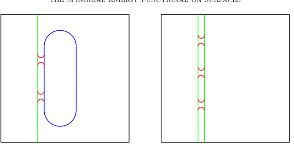
In the higher genus case we use the tori Tb andTn constructed above as building blocks which we connect by handles with small Willmore energy. The construction is illustrated in Fig. 1. Ifσis a non-bounding spin structure, we align a copy ofTn and a copy of Tb in such a way that Tn is parallel and at small distance to a flat
Figure 1. Surfaces with almost minimisers. The left-hand picture shows a torus with a non-bounding spin structure, drawn in green, and a torus with a bounding spin structure, drawn in blue. These surfaces are connected by necks drawn in red. The right-hand picture shows two tori with a non-bounding spin structure, drawn in green, connected by necks drawn in red.
disk insideTb. Then we connect Tn and Tb by γ−1 handles. If σ is a bounding spin structure, we take two parallel copies ofTnat small distance, and call themTn′ andTn′′. Then we connectTn′ andTn′′ byγ−1 handles. According to Lemma 3.10 this can be done without introducing more than an arbitrarily small amount of Willmore energy. The resulting surface has genus γ and carries a non-bounding spin-structure in the first, and a bounding spin structure in the second case.
We return to the proof of Theorem 3.9. With the notations of the lemma and the proposition we setg∶=F∗(g0). Further, we restrict a parallel spinor of unit length onT3 to F(Mγ)and pull it back to a spinorϕon(Mγ, σ, g). As in [7] it follows thatDϕ=Hϕ, whence
1 2∫M
γ
∣Dϕ∣2dvg= 1 2∫M
γ
H2dvg= W(F) ≤ε and thus
E(g, ϕ) = 1 2∫M
γ
∣Dϕ∣2−1 4∫M
γ
K≤ε−π
2χ(M) =ε+π∣γ−1∣
as claimed.
From (18), the Lichnerowicz-Weitzenb¨ock formula and the results from Section 2.4 we immediately deduce the
Corollary 3.13. Ifγ≥1, thenE(g, ϕ) =π∣γ−1∣ if and only if Dgϕ=0, that is,ϕ is a harmonic spinor of unit length. In particular, absolute minimisers of E over Mγ correspond to minimal isometric immersions of the universal covering ofMγ. Remark 3.14. In the case of the sphere (γ =0) equality holds if and only if ϕ is a so-calledtwistor spinor, see Section 4. Furthermore, as a consequence of the Lichnerowicz-Weitzenb¨ock and Gauss-Bonnet formula, a unit spinor on the torus (γ=1) is harmonic if and only if it is parallel.
Example 3.15. For any γ ≥ 3 there exists a triply periodic orientable minimal surfaceM inR3such that if Γ denotes the lattice generated by its three periods, the projection ofMto the flat torusT3=R3/Γ isMγ [14, Theorem 1]. Since the normal bundle of Mγ in T3 is trivial there exists a natural induced spin structure which we claim to be a bounding one. To see this we need to analyse the construction in [14] which is a refinement of the construction used in Lemma 3.12. In a first step one starts with two flat minimal 2-dimensional tori T1 andT2 inside the flat 3-dimensional torusT3. One can assume thatT1 and T2 are parallel. The trivial spin structure onT3admits parallel spinors which we can restrict to parallel spinors onT1andT2. In particular, bothT1andT2 carry the non-bounding spin structure so that the disjoint unionT1∐T2carries a bounding spin structure. Namely,T1∐T2 is the boundary of any connected component ofT3∖ (T1∐T2), and this even holds in the sense of spin manifolds, cf. also the discussion in [12, Remark II.2.17]. In a second step, small catenoidal necks are glued in between T1 and T2 but this does not affect the nature of the spin structure which thus remains a bounding one.
Using the conformal equivariance (9) of the Dirac operator gives a further corollary.
Namely,E(g, ϕ) =π(γ−1)for(g, ϕ) ∈ N if and only if there is metric ˜gwith nowhere vanishing spinor ˜ϕwithD˜gϕ˜=0. Indeed, forg= ∣ϕ˜∣4˜g˜gthe rescaled spinorϕ=ϕ˜/∣ϕ˜∣g is in the kernel ofDg and of unit norm.
Corollary 3.16. For γ ≥ 1 absolute minimisers on a spin surface correspond to nowhere vanishing harmonic spinors on Riemann surfaces.
Example 3.17. Concrete examples can be constructed from the holomorphic de- scription of harmonic spinors in Section 2.1. Consider a surface of genus γ ≥ 2 with a hyperelliptic complex structure. These are precisely the complex structures for which the Riemann surface arises as a two-sheeted branched coverings of the complex projective line (see for instance [10, Paragraph §7 and §10]). There are exactly 2(γ−1)branch pointsw1, . . . , w2(γ+1), the so-calledWeierstraß points. For any Weierstraß point w, the divisor 2(γ−1)w defines the canonical line bundle κ of Mγ, and λ defined by (γ−1)w is a holomorphic square root. In particu- lar, there exists a holomorphic sectionϕ0 ∈H0(Mγ,O(λ)) – a positive harmonic spinor – whose divisor of zeroes is precisely(γ−1)w, that is,ϕ0 has a unique zero of order γ−1 atw. Furthermore, on hyperelliptic Riemann surfaces there exists a meromorphic function f on M with a pole of order 2 at w and a double zero elsewhere, say at p∈ M. Hence, if the genus of M is odd, then ϕ1 = f(γ−1)/2ϕ0
is a holomorphic section which has a unique zero at p. Regarding ϕ1 as a nega- tive harmonic spinor via the quaternionic structure therefore gives a non-vanishing harmonic spinor ϕ0⊕ϕ1∈Γ(Σg). Rescaling by its norm gives finally the desired absolute minimiser. Note that dimCH0(Mγ,O(λ)) = (γ+1)/2 (see for instance [10, Theorem 14]) so thatλcorresponds to a non-bounding spin structure ifγ≡1 mod 4, and to a bounding spin structure ifγ≡3 mod 4.
On the other hand, there are also obstructions against attaining the infimum.
Lemma 3.18. If (g, ϕ)is an absolute minimiser over Mγ with γ≥2, thend(g) = dimCkerDg≥4.
Proof. As noted in Section 2.3, d(g) is even, so it remains to rule out the case d(g) =2. Viewing ΣM →M as a quaternionic line bundle with scalar multiplication from the right, kerDg inherits a natural quaternionic vector space structure. In
particular, it is a 1-dimensional quaternionic subspace ifd(g) =2. SinceD(1+iω)ϕ= Dϕ−iωDϕ=0 there is a quaternionqwith(1+iω)ϕ=ϕq. Ifq≠0, then(1+iω)ϕ is a nowhere vanishing section of the complex line bundle Σ+ and thus yields a holomorphic trivialisation of the holomorphic tangent bundle via the holomorphic description of harmonic spinors in Section 2.1. In particular,γ=1. Ifq=0, thenϕ is a nowhere vanishing section of Σ−≅Σ+and a similar argument applies.
Summarising, we obtain the following theorem concerning existence respectively non-existence of absolute minimisers.
Theorem 3.19. On(Mγ, σ)the infimum of E (i) is attained in the cases
(a) γ=1 andσis the non-bounding spin structure.
(b) γ≥3 andσis a bounding spin structure.
(c) γ≥5 withγ≡1 mod 4 andσis a non-bounding spin structure.
(ii) is not attained in the cases
(a) γ=1 andσis a bounding spin structure.
(b) γ=2
(c) γ=3,4 andσis a non-bounding spin structure.
Remark 3.20.
(i) It remains unclear whether the infimum is attained for a non-bounding spin structure on surfaces of genus γ≥6 andγ/≡1 mod 4.
(ii) In the case of the sphere (γ= 0) the infimum of E is always attained. This will be discussed in Section 4.
Proof of Theorem 3.19. (i) The non-bounding spin structure onT2is the one which admits parallel spinors, while (b) and (c) follow from Example 3.15 and Exam- ple 3.17 respectively.
(ii) From Section 2.3 we know thatd(g)must be divisible by 4 ifσis bounding while from Hitchin’s boundd(g) ≤γ+1 [11]. Therefore, under the conditions stated in (a) or (b),d(g) ≤3 for any metricg onMγ so that for a boundingσwe necessarily have d(g) =0. If γ ≥ 2 we have d(g) ≥4 by Section 2.3 and moreover, d(g) ≡ 2 mod 4 ifσis non-bounding. Hence d(g) ≥6 which is impossible ifγ≤4.
Finally, we characterise the absolute minimisers in terms ofAandβ. First we note thatJ induces a natural complex structure onT∗M⊗T M defined by
i(α⊗v) =iα⊗v=α⊗iv∶=α⊗J v.
Equipped with this complex structure, T∗M ⊗T M becomes a complex rank 2 bundle, and we have the complex linear bundle isomorphism
T∗M⊗T M ≅T M1,0⊗C(T∗M⊗C), α⊗v↦α⊗ 12(v−iJ v). (20) In this way, considering Aas a T M-valued 1-form, the decomposition Ω1(T M) ≅ Ω1,0(T M1,0) ⊕Ω0,1(T M1,0)gives a decomposition
A=A1,0+A0,1.
Since T∗M1,0⊗CT M1,0 is trivial we may identify A1,0 with a smooth function f ∶M →C. Further, on any K¨ahler manifoldT M0,1≅T∗M1,0 so we may identify A0,1 with a quadratic differential q ∈Γ(κ2γ). Finally, ¯∂f ∈Ω0,1(Mγ) ≅Γ(T Mγ1,0) and ¯∂q∈Ω0,1(κ2γ) ≅Γ(T Mγ0,1).
Lemma 3.21. Modulo these isomorphisms we have
−1
2divA1,0=∂f¯ and −1
2divA0,1=∂q.¯
In particular,divA1,0=0if and only if∂f¯ =0anddivA0,1=0if and only if∂q¯ =0.
Proof. If we write
A= (a c b d)
in terms of a positively oriented local orthonormal frame{ei}, then A1,0= (α −β
β α) =12(a+d −b+c
b−c a+d), A0,1= (γ δ
δ −γ) = 12(a−d b+c
b+c −a+d). (21) HenceA1,0is the sum of the trace and skew-symmetric part ofA, whileA0,1 is the traceless symmetric part of A. Now fix a local holomorphic coordinatez =x+iy and assume that{ei}is synchronous atz=0, i.e.e1(0) =∂x(0)ande2(0) =∂y(0). In particular, ∂z = (∂x−i∂y)/2 corresponds to e1 under the identification (20).
From (21)
A1,0= (α+iβ)dz⊗∂z and A0,1= (γ−iδ)dz⊗∂z¯, whencef =α+iβ andq= (γ−iδ)dz2. Then atz=0,
divA1,0= (−e1(α) +e2(β))e1− (e2(α) +e1(β))e2
and
divA0,1= −(e1(γ) +e2(δ))e1+ (e2(γ) −e1(δ))e2.
Computing ¯∂f =∂¯z(α+iβ)d¯z and ¯∂q =∂z¯(γ−iδ)d¯z⊗dz2 gives immediately the
desired result.
Remark 3.22. In particular, for a critical point(g, ϕ)the symmetric(2,0)-tensor associated with A0,1 is a tt-tensor, that is, traceless and transverse (divergence- free). Forγ≥2, the previous lemma therefore recovers the standard identification of the space of tt-tensors with the tangent space of Teichm¨uller space given by holomorphic quadratic differentials.
We are now in a position to give an alternative characterisation of absolute min- imisers ifγ≥1. The case of the sphere will be handled in Theorem 4.6.
Proposition 3.23. Let γ≥1. The following statements are equivalent:
(i) (g, ϕ)is an absolute minimiser.
(ii) ∇Xϕ=A(X) ⋅ϕ for a traceless symmetric endomorphismA.
(iii) (g, ϕ)is critical andβ=0.
Remark 3.24. In particular, we recover the equivalence (ii)⇔(iii) of [7, Theorem 13] for the caseH =0.
Proof. By Theorem 3.9, (g, ϕ) is an absolute minimiser if and only if Dϕ = 0.
From (8) this is tantamount to TrA = 0, Tr(A○J) = 0 and β = 0. The trace conditions are equivalent toAbeing symmetric and traceless whence the equivalence between (i) and (ii). Furthermore, (ii) immediately forces β =0. Conversely, (iii) together with the critical point equation in Proposition 3.1 implies 2AtA= ∣A∣2Id, whence 2∣A∣2= ∣K∣ by Corollary 3.7 (i). In particular, 2∣A∣2= −K on the open set U = {x∈Mγ ∶K(x) <0}. Assume thatU is non-empty and not dense in Mγ, i.e.
U¯ ⊂ Mγ∖ {p} for some p ∈ Mγ. Without loss of generality we may also assume
U to be connected. On its boundary the curvature vanishes so that in particular,
∣A∣ =0 on ∂U. Further, ∣Dϕ∣2= ∣A∣2+K/2 =0 on U as a simple computation in an orthonormal frame using Eq. (8) reveals. As before, Dϕ=0 implies that A is traceless symmetric and divergence-free overU. In particular,A corresponds to a holomorphic quadratic differential by Lemma 3.21. Since every holomorphic line bundle on the non-compact Riemann surface Mγ ∖ {p} is holomorphically trivial (see for instance [5, Theorem 30.3]), overU the coefficients ofAarise as the real and imaginary part of a holomorphic function and are therefore harmonic. However, they are continuous on ¯U and vanish on the boundary, henceA=0 by the maximum principle. In particular, K = 0 on U, a contradiction. This leaves us with two possibilities. EitherU is dense inMγ orU is empty. By Gauss-Bonnet the second case can only happen for genus 1 and gmust be necessarily flat. In any case, ϕis harmonic and therefore defines an absolute minimiser.
Corollary 3.25. Let γ ≥ 1. If (g, ϕ) is an absolute minimiser, then A is a tt- tensor. Furthermore, K ≡0 if γ =1 and K ≤0 with only finitely many zeroes if γ≥2.
Remark 3.26.
(i) As we will see in Section 5 there exist flat critical points which are not absolute minimisers.
(ii) Ifγ≥2 in Proposition 3.23 (iii), it suffices to assume that∣β∣ =const. Indeed, (β⊗β)0induces a holomorphic section ofκ2γand has therefore at least one zero.
At such a zero,(β⊗β)0=0, henceβ=0 in this point and thus everywhere.
(iii) Ifβ=0, then Proposition 3.8 implies div(A○J) =0. However, this does not yield an extra constraint as div(A○J) =divAforAsymmetric.
4. Critical points on the sphere
In this section we completely classify the critical points in the genus 0 case where Mγ is diffeomorphic to the sphere. In particular, up to isomorphism there is only one spin structure forS2 is simply-connected.
4.1. Twistor spinors. For a general Riemannian spin manifold (Mn, σ, g) with spinor bundle ΣgMn→Mn, aKilling spinorϕ∈Γ(ΣgMn)satisfies
∇Xψ=λX⋅ψ
for any vector fieldX ∈Γ(T M)and some fixedλ∈C, the so-calledKilling constant.
In particular, the underlying Riemannian manifold is Einstein with Ric =4λ2g so that λ is either real or purely imaginary. If M is compact and connected, only Killing spinors ofreal type, whereλ∈R, can occur [4, Theorem 9 in Section 1.5].
More generally we can consider twistor spinors. By definition, these are elements of the kernel of the twistor operatorTg=prkerµ○ ∇, where prkerµ∶Γ(T∗M ⊗Σ) → Γ(kerµ)is projection on the kernel of the Clifford multiplicationµ∶T∗M⊗ΣM → ΣM. Equivalently, a twistor spinor satisfies
∇Xϕ= −n1X⋅Dϕ
for all X∈Γ(T M). The subsequent alternative characterisation will be useful for our purposes.