Joint stochastic constraint of a large data set from a salt dome

(1)

Joint stochastic constraint of a large data set from a salt dome

Alan W. Roberts

¹

, Richard W. Hobbs

²

, Michael Goldstein

³

, Max Moorkamp

⁴

, Marion Jegen

⁵

, and Bjørn Heincke

⁶

ABSTRACT

Understanding the uncertainty associated with large joint geophysical surveys, such as 3D seismic, gravity, and magnetotellu- ric (MT) studies, is a challenge, conceptually and practically. By demonstrating the use of emulators, we have adopted a Monte Carlo forward screening scheme to globally test a prior model space for plausibility. This methodology means that the incorpo- ration of all types of uncertainty is made conceptually straightforward, by designing an appropriate prior model space, upon which the results are dependent, from which to draw candidate models. We have tested the approach on a salt dome target, over

which three data sets had been obtained; wide-angle seismic refraction, MT and gravity data. We have considered the data sets together using an empirically measured uncertain physical relationship connecting the three different model parameters: seismic velocity, density, and resistivity, and we have indicated the value of a joint approach, rather than considering individual parameter models. The results were probability density functions over the model parameters, together with a halite probability map. The emulators give a considerable speed advantage over running the full simulator codes, and we consider their use to have great potential in the development of geophysical statistical constraint methods.

INTRODUCTION

To map a region of earth, it is commonplace to use one or more kinds of data sets to constrain structural models parameterized by one or more proxy parameters, such as seismic velocity, density, or resistivity. An interpreter will then use their geologic insight com- bined with these models to make judgments about the region. This may be with a view to, for example, determining where appropriate drilling locations might lie to maximize the possibility of hydrocarbon extraction. There are many approaches used to constrain the proxy models, ranging from deterministic inverse approaches to Markov chain Monte Carlo (MCMC) search schemes (Press, 1970;

Sambridge and Mosegaard, 2002;Shapiro and Ritzwoller, 2002;

Hobro et al., 2003; Gallardo and Meju, 2004;Roy et al., 2005;

Heincke et al., 2006;Meier et al., 2007;Moorkamp et al., 2011).

Deterministic inverse schemes are optimal when the uncertainties in

the data and physical system are small, and the aim is to find the optimum model as fast as possible. This approach works by repeated model update so as to minimize the difference between the observed data and the simulator’s output. However, in many scenar- ios, there are considerable uncertainties associated with the data and physics concerned. In this case, statistical schemes may be adopted.

In these methods, the aim is normally to discern the entire plausible model space for the system concerned. The character of such statistical schemes varies from the entirely forward-based screening method (Press, 1970), to the more targeted sampling strategy of the MCMC approach (Hastings, 1970; Sambridge and Mosegaard, 2002). MCMC schemes seek to sample enough of the model space to give a robust uncertainty estimate; however, often, the number of forward simulations in both of these methods required to sufficiently sample the space for large systems often makes these methods computationally impracticable. Thus, often in part due to the

Manuscript received by the Editor 27 February 2015; revised manuscript received 21 August 2015; published online 19 February 2016.

1Formerly Durham University, Department of Earth Sciences, Durham, UK, and Durham University, Department of Mathematics, Durham, UK; presently Geospatial Research Limited, Durham, UK. E-mail: a.w.roberts@durham.ac.uk.

2Durham University, Department of Earth Sciences, Durham, UK. E-mail: r.w.hobbs@durham.ac.uk.

3Durham University, Department of Mathematics, Durham, UK. E-mail: michael.goldstein@durham.ac.uk.

4Formerly GEOMAR, Kiel, Germany; presently University of Leicester, Department of Geology, Leicester, UK. E-mail: mm489@leicester.ac.uk.

5GEOMAR, Kiel, Germany. E-mail: mjegen@geomar.de.

6Formerly GEOMAR, Kiel, Germany; presently GEUS, Department of Petrology and Economic Geology, Copenhagen, Denmark. E-mail: bhm@geus.dk.

ID1

10.1190/GEO2015-0127.1

Downloaded 03/17/16 to 129.234.252.65. Redistribution subject to SEG license or copyright; see Terms of Use at http://library.seg.org/

(2)

lack of a feasible method of assessing the uncertainty associated with a system and also conceptual difficulties in incorporating a particular kind of uncertainty into the constraint process, the uncertainty assessments that are fed into the decision-making processes can be ill informed.

The approach adopted here is a forward-modeling-based screening strategy. To make the process computationally feasible, we build

“emulators”for each of the forward modeling (“simulator”) codes, trained over the prior model space. We use the termemulatorto mean a statistical model of the output generated by a complex forward modeling code, orsimulator. The aim of building an emulator is to have a means of generating a fast uncertainty calibrated estimate of the simulator output (which maybe be time expensive to compute). Through providing uncertainty-calibrated rapid estimates of the full simulator output, these emulators overcome the computational barrier of making vast numbers of complex simulator runs.

By iteratively rejecting an implausible model space and updating the emulators, the plausible model space is discerned. In this study, we apply the method to constrain a region of earth characterized by a salt dome using three kinds of data: seismic refraction, magneto- telluric (MT), and gravity data sets for a 1D seven-layered parameterization, and we construct a rock-type probability map based on the fractional salt versus sediment model acceptance for the region. As discussed inOsypov et al. (2011)and elsewhere, proper assessment of risk in hydrocarbon exploration requires not only the analysis of a proxy-parameter model, but also a full analysis of the structural uncertainty. The ability to construct a probability map in this manner has the potential to be of considerable value in this regard.

Joint inversion

Deterministic inversion methods (Tarantola, 2005), in which the aim is to iteratively update a model so as to reduce some objective function, are commonly used when the data come from a single technique. However, using such schemes in a joint framework in which the relationship between the physical parameters (e.g., seismic velocity, resistivity, and density) is empirical and uncertain, poses philosophical challenges regarding the coupling strategy, for example, the weighting attached to maintain structural coher- ency across the various methods (Gallardo and Meju, 2004). Sim- ilarly, there are also conceptual intricacies associated with properly and quantitatively including most kinds of uncertainty associated with the problem, for example, uncertainty in the data measurements and model discrepancy (due to the fact that a model is not a complete representation of nature). Recently however, a few au- thors such asRoy et al. (2005),Heincke et al. (2006), andMoor- kamp et al. (2011,2013)make considerable progress in developing structural coupling-based joint inversion methodologies through crossgradient and other coupling schemes.Bodin et al. (2012)also develop hierarchical Bayes approaches for joint inversion.

Statistical schemes

Statistical schemes designed to assess uncertainty, such as simulated annealing, genetic algorithms, and MCMC approaches, can be used when the number of model parameters is small.Sambridge and Mosegaard (2002)give a useful review of the varied methods that can be used and their historical development.

However, as is commented inSambridge and Mosegaard (2002), if the number of parameters is large, then these methods become

unfeasible because the number of complex, and possibly expensive, forward model simulations becomes impracticably large given the computation time required. In a few scientific fields, such as clima- tology, volcanic hazard prediction, ocean modeling, and cosmology (Logemann et al., 2004;Rougier, 2008;Bayarri et al., 2009;Vernon and Goldstein, 2009), in which forward simulators are also highly time expensive to run,emulatorsare often used. An emulator is a statistical representation of the forward modeling simulator, which gives a very rapid prediction of the simulator output, with a calibrated uncertainty.

Building an emulator is similar to building a neural network.

Neural networks are successfully used to solve inverse problems in geophysics, for example,Meier et al. (2007), who develop a neural network system to invert S-wave data. Others have also devel- oped methods of using quick approximations to a full forward code in inversion schemes, for example,James and Ritzwoller (1999), who use truncated perturbation expansions to approximate Ray- leigh-wave eigenfrequencies and eigenfunctions, andShapiro and Ritzwoller (2002), who take a similar methodology in an MCMC scheme to construct a global shear-velocity model of the crust and upper mantle. In each of these cases, the aim is to minimize some objective function or maximize a likelihood function.

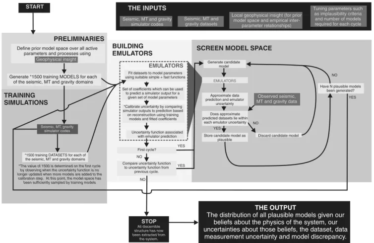
Here, we adopt a statistical approach that is fundamentally different in that it is based entirely on forward modeling, as opposed to using any kind of objective/likelihood function or inverse step. We simply seek to discern which areas of model space are plausible and which are implausible, given the observed data. This approach has been proposed in the past (e.g.,Press, 1970), and it is used in a variety of settings such as the history matching of hydrocarbon reservoir pro- duction data (Murtha, 1994;Li et al., 2012). However, in the context of structural constraint, it is largely sidelined in favor of more search- efficient schemes such as those described above. We implement this forward approach by the use of emulators to make it more computationally efficient.Roberts et al. (2012)describe our methodology for a synthetic scenario; however, here we describe a number of mod- ifications to achieve greater stability and efficiency. We develop and apply the approach to observed 3D joint seismic, MT, and gravity data sets obtained from a salt dome region, and we ultimately determine a model probability map for the profile. The method is akin to the response surface methodologies beginning to be used in the field of reservoir simulation (Zubarev, 2009). However in this case, we seek to fully model the uncertainty in the simulator-prediction system, and hence we aim to construct response clouds, rather than sur- faces. The method is shown diagrammatically in Figure1.

The strategy here, to exclude model space, rather than build up the plausible space searching from some starting model, represents a fundamentally and philosophically different “top-down” approach, to the traditional inversion, and it relies entirely on forward computation. Because we globally sample the prior plausible model space, seeking to exclude implausible model space, rather than searching a part of the model space for plausible models, the uncertainty measures which are obtained are maxima, rather than min- ima, given the prior model space and choices of tuning parameters made in the analysis.

Building statistical system models, oremulators, successively in a multicycle fashion, we progressively refine the plausible space.

Because a proper consideration of uncertainty in an inverse scheme can be conceptually difficult, often, when any consideration of uncertainty is made, it is commonly specified to be Gaussian in

Downloaded 03/17/16 to 129.234.252.65. Redistribution subject to SEG license or copyright; see Terms of Use at http://library.seg.org/

(3)

character at times not because it is indeed Gaussian, but simply because of mathematical convenience. The fact that, in our method, the screening process relies entirely on forward modeling means that it is conceptually straightforward to include uncertainty pertain- ing to any part of the system by building the appropriate distribution over the prior model space. These uncertainties may take the form of data uncertainty, physical uncertainty, model discrepancy, or others, which in an inversion scheme, including physical uncertainties and model discrepancy, among others, can be conceptually difficult.

Emulation

To overcome computational limitations in our forward screening Monte Carlo scheme, we build and use emulators (Kennedy and O’Hagan, 2001;Vernon et al., 2009). Like the case of a neural network, an emulator is designed using training models and data sets, and it seeks to predict the output data arising for a given model parameter set. However, an emulator differs from a neural network in that it seeks to not only predict the output of a system from an input, but also to do so with a fully calibrated uncertainty. An emulator treats the parametric and nonparametric parts of the system holistically, giving a full stochastic representation of the system.

Because of this focus on uncertainty calibration, emulators can be used to rapidly screen model space for implausibility (Goldstein and Wooff, 2007). This would not be the case with an uncalibrated simulator-prediction system because there is no measure or criterion to discern whether a comparative data set is sufficiently close to the

observed data set to be deemed plausible. Although the method described here is very much a forward modeling philosophy, in that we are simply seeking to trial sets of model parameters for plausibility, one could consider that the fitting of parametric functions to build the emulator model of the forward simulator constitutes a partly inverse component. However, because the forward simulator itself, rather than the model parameters is being“inverted”for, the emulator screening method is fundamentally different to a traditional inversion scheme.

Although there are occasional instances of emulators being de- veloped for earth systems (Logemann et al., 2004), they have not been widely applied in the geosciences. Here, we review and dem- onstrate the use of an emulator (Roberts et al., 2010,2012) to constrain the structure of a salt diapir using 1D profiles through a 3D joint data set. Figure1summarizes the strategy adopted in this study.

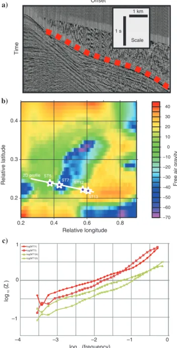
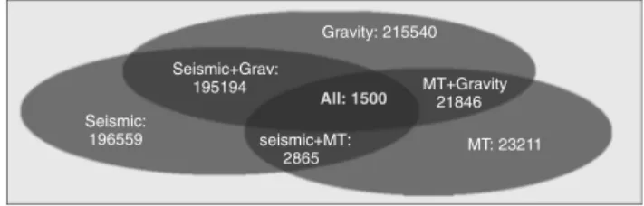
The data consist of 3D seismic data, full tensor gravity (FTG) data, and MT data from a salt dome. Examples from the three data sets are shown in Figure2.

THEORY AND PRELIMINARIES

In performing an experiment to test a model, the scientist has a set of output data points, a set of model parameters, and a function (simulatoror forward modeling code)f, which defines the relationship between the model parameters θ and the “perfect” data ψ (equation1) as follows:

Fit datasets to model parameters using suitable simple + fast functions

*Calibrate uncertainty by comparing simulator outputs to prediction based on reconstruction using training

models and fitted coefficients Set of coefficients which can be used

to predict a simulator output for a given set of model parameters

Uncertainty function associated with emulator prediction

EMULATORS Generate candidate model

EMULATORS

Approximate data prediction and emulator

uncertainty

Does approximate predicted datasets lie within

each emulator uncertainty

Store candidate model as plausible YES

Discard candidate model

Have N plausible models been generated?

NO

YES

Compare uncertainty function to uncertainty function from

previous cycle.

First cycle?

YES

NO

STOP

All discernible structure has now been extracted from

the system.

START

YES

NO Seismic, MT, gravity

simulator codes

Define prior model space over all active parameters and processes using

Generate *1500 training MODELS for each of the seismic, MT and gravity domains

*1500 training DATASETS for each of the seismic, MT and gravity domains

*The value of 1500 is determined on the first cycle by observing when the uncertainty function is no longer updated when more models are added to the

calibration step. At this point, the model space has been sufficiently sampled by training models

NO

THE OUTPUT

The distribution of all plausible models given our beliefs about the physics of the system, our uncertainties about those beliefs, the dataset, data

measurement uncertainty and model discrepancy.

PRELIMINARIES

TRAINING SIMULATIONS

BUILDING

EMULATORS SCREEN MODEL SPACE THE INPUTS

Seismic, MT and gravity simulator codes

Seismic, MT and gravity datasets

Observed seismic, MT and gravity data Geophysical insight

Local geophysical insight (for prior model space and empirical inter-

parameter relationships)

Tuning parameters such as implausibility criteria and number of models required for each cycle

Figure 1. The emulator screening methodology.

Downloaded 03/17/16 to 129.234.252.65. Redistribution subject to SEG license or copyright; see Terms of Use at http://library.seg.org/

(4)

ψ¼fðθÞ: (1) In the case of a heavily parameterized system, with many nodes in the parameter models, and many output data, this function, or simulatorfcan take a long time to evaluate. For a typical inversion problem involving seismic data, many thousands of evaluations off

maybe required, and the problem very quickly becomes impractical to solve if the time spent evaluatingf is significant.

Vernon et al. (2009)andKennedy and O’Hagan (2001)use emulators to address this kind of problem in which large numbers of complex simulator evaluations are required. An emulator seeks to represent the simulator functionfas a combination of a computationally cheap deterministic function (e.g., a polynomial)hand a Gaussian process g(Rasmussen and Williams, 2010):

ψ¼hðθÞ þgðθÞ: (2)

The aim is not to completely replace the full simulator, but to develop a system such that one can very quickly glean enough information from the relationship between the model parameters and output data to make meaningful judgments about whether regions of model space can be excluded from the analysis on the basis that they would result in output data not compatible with the observed data.

Becausehandgare fast to evaluate, a considerable time savings (of orders of magnitude) can typically be achieved by this approach.

In the study detailed here, we adopt a multistage approach (Vernon et al., 2009) of seeking to describe the global behavior and then, as the implausible model space is excluded, to describe increasingly localized behavior as we develop more predictively accurate emulators.

DATA, MODEL SPACE, AND THE INVERSE PROBLEM

Data

A joint data set for this study was kindly supplied by Statoil. It is a joint 3D seismic, FTG and MT data set recorded over a region known to Statoil as being characterized by a salt diapiric body (Fig- ure2). To simplify the problem, we enforce a local 1D solution. The MT data were transformed into the directionally independent Ber- dichevsky invariant form (Berdichevsky and Dmitriev, 2002), seismic data were picked for 1868 shot gathers and transformed into the common midpoint (CMP) domain, and the closest CMP profiles to each MT station were identified and used as 1D seismic data for the purposes of the study. The FTG data were transformed to scalar data, and the closest measurement to each MT station was identified. Results are thus generated for the series of 1D seismic, MT, and gravity data sets collocated at the site of each MT station. In this paper, each site is labeled “STxx”, where“xx” can take the value 1–14, for example, in Figure2.

Gravity datum

In addition, it was also necessary to establish a datum for the gravity data measurements so as to make meaningful comparison between each station. This is because if the models are allowed to be of arbitrary total thickness, then the gravity reading could be considered as simply as a free parameter and afford no constraint.

In practice, this is an expression of the Airy hypothesis of isostasy (Airy, 1855). This calibration requires the tying of the measured gravity point at one station to the simulator output at that station, with an assumption about the structure at that station, against which results at the other stations can be considered as being relative to. This assumption might be that the model is of a given total Offset

Time

1 km

1 s Scale

a)

log(MT7r) log(MT7i) log(MT12r) log(MT12i)

log (frequency)10

log(Z)10

–4 –3 –2 –1 0

0

–1

c) 1 0.2 0.3 0.4

Relative latitude

0.2 0.4 0.6 0.8

Relative longitude

ST7 ST12

–70 –60 –50 –40 –30 –20 –10 0 10 20 30 40

Free air gravity ST5

ST13

b)

2D profile

Figure 2. Data examples: (a) seismic, (b) gravity, and (c) MT. The red dots on the seismic gather show the first arrival wide-angle turn- ing waves, which are being modeled in this study. On the gravity map in panel (b), the locations of ST5, ST7, ST12, and ST13 (which are frequently referred to in this study) are marked with purple stars, and the track of the 2D line for which profiles are shown in later figures. The MT data plot shows Berdichevsky invariant (Berdi- chevsky and Dmitriev, 2002) Re(Z) and Im(z) for stations ST7 (red) and ST12 (green).

Downloaded 03/17/16 to 129.234.252.65. Redistribution subject to SEG license or copyright; see Terms of Use at http://library.seg.org/

(5)

thickness, or some other consideration about the model. We choose to use the assumption that at a given point along the line, there is no salt present. On the grounds that prior studies indicate that it lies over a region of sediment, we chose to use station ST12 (Figure2) for the purpose of gravity calibration. The calibration was carried out by running the code with gravity screening disabled, only generating “sediment models” and then generating density models using the relationship in equation7from the plausible velocity models. Gravity measurements were then generated from these models using the gravity simulator, and the most likely gravity measurement were compared with the measured gravity value at station ST12. The difference between these two values was then used as a“correction”value for comparing screened gravity values to measured gravity values at all the other stations. In practice, this means that the gravity results in this study and the“salt content”are being measured relative to station ST12 screened with the assumption that there is no salt there (the prior probability of salt in each layer is set to zero, and thus no salt models are generated). However, for a meaningful comparison (and a test of the assumption that there is no salt at ST12), the screening process is then repeated for ST12 with the possibility of salt models included with a probability of 0.5 in each layer, as was the case for the other stations. A comparison of the results prior to the gravity calibration (without gravity constraint) and postcalibration (the main results presented in this paper) would provide an interesting study; however, for brevity, these pre- liminary outputs are not discussed here.

Methods and model space

Our goal is to describe the model in terms of proxy quantities (P-wave velocity, resistivity, and density) and also to obtain a rock probability map for the profile along which the MT stations are located. Although the priors in this study are somewhat illustrative, in a scenario in which the priors are well constrained and tested, such a probability map may be used as a more direct input to evaluate geologic risk, rather than simply providing proxy-parameter models that the scientist must then interpret. We discern the distribution of jointly plausible models with respect to each of the seismic, gravity, and MT data sets, given all of the uncertainties we wish to specify, by generating candidate joint models drawn from a prior model space. In this way, we effectively screen the model space using the interparameter relationship to discriminate between salt and sediment rocks.

As is noted inRoberts et al. (2012), the simulators, particularly the seismic simulator (Heincke et al., 2006), are more sophisticated than required for the problem at hand; however, to facilitate future development and allow integration and direct comparison with other work (Heincke et al., 2006;Moorkamp et al., 2011,2013), we use these simulators.

Prior model space

The first consideration is the initial model space within which we consider the plausible models for the system to lie (Figure1). Our focus here is on the emulation methodology as a means to screen and constrain model space, rather than on generating robust Baye- sian posterior distributions for the particular region used for the case study. As such, here we have placed only a cursory emphasis on the determination and specification of the prior model space. The final result should, therefore, not be considered as a true Bayesian constraint from which a genuine geologic inference can be made about

this region. For such a result, proper consideration of appropriate priors should be made, and proper sensitivity calibration through sampling those priors. Accordingly, the analysis presented here is made on the assumption that there is indeed halite present in the region of earth under consideration and on the basis that that halite, and indeed the surrounding material, has properties reflective of those seen globally and in conjunction with the borehole data set described below.

Similarly, at several points in the emulator building and screening process, the tuning parameters are set. Again, here these are chosen somewhat qualitatively and arbitrarily. In reality, the choices made for these parameters also constitute part of the model space, and so for the results of the screening process to be geologically meaningful, expert judgment should be used in the choice of these parameters, with a prior distribution that can be fully sampled. The final results of the analysis presented here should thus be treated as being illustrative of the method and should be subject to all of the explicit and implict assumptions made, rather than being authoritative as to the earth structure in question.

Our prior joint model space is constrained primarily by three influences: (1) the interparameter relationship linking the seismic velocity, density, and resistivity parameters, (2) the range of geo- physically plausible values which each of these parameters may adopt, and (3) the prior probability of salt existing in each layer.

Physical parameter relationship.—For the purpose described here, a rock is characterized by its combination of physical properties (in our case, resistivity, seismic velocity, and density), which are encap- sulated by the empirical physical parameter relationships that connect them. In this joint setting, we therefore propose, for a given layer, combinations of model parameters across each of the domains that are con- nected by either a sediment relationship or a“salt relationship. By doing this, and then assessing the fraction of models deemed plausible generated using each relationship for a given depth, we can then make a statement about the rejection ratio for models generated using each relationship regarding the probability that salt or sediment exists at different locations and constructing a salt likelihood map for the profile.

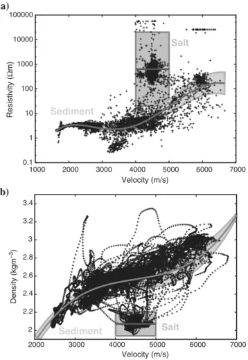
The interparameter relationship for sediments, although it is empirical and uncertain, may be relatively easily formulated by fitting a curve through well-log data from the survey area (Figure3). How- ever, the presence of salt complicates the situation somewhat, in that for sediment there is a monotonic increase between seismic velocity, density, and resistivity. However, salt has a very characteristic seismic velocity of 4500 m∕s, a density of around2100 kg∕m³ (Birch, 1966), and very high resistivity (>500Ωm;Jegen-Kulcsar et al., 2009). Therefore, we define two relationships for our situation, as shown in equations5–9. In this case, we have chosen the uncertainty to be a function added to a central value. It would also be straightforward to specify the uncertainty in other ways, for example, as uncertainty in the values of the relationship coefficients.

In these relationships,r,ρ, andvrefer to the resistivity, density, and seismic velocity values, respectively. The valueNða; bÞrefers to a sample from a normal distribution of meanaand standard deviation b. The borehole data from which the sediment density/resistivity/

velocity relationship was obtained (kindly provided by Statoil) is shown in Figure 3. The borehole is located adjacent to station ST5 (Figure2). Consideration of Figure3suggests that given that there are a considerable number of points lying outside the bounds shown for the salt and sediment relationships, there may be a case

Downloaded 03/17/16 to 129.234.252.65. Redistribution subject to SEG license or copyright; see Terms of Use at http://library.seg.org/

(6)

for including a third relationship category of“other,”to accommo- date these currently extremal points more effectively. However, for simplicity, here we decided to continue with the two-relationship scheme. In this case, we have used data from this single borehole for the entire line. A more rigorous study would seek if possible to consider borehole data from various points along the line to account for regional variation.

Sediment parameter relationships are given in the following equations:

log₁₀ðrÞ ¼−8.72487þ0.0127274v−6.4247×10⁻⁶v²

þ1.45839×10⁻⁹v³; (3)

−1.47131×10⁻¹³v⁴þ5.32708×10⁻¹⁸v⁵þNð0;σrðvÞÞ; (4)

σrðvÞ ¼−2.931×10⁻²þ1.989×10⁻⁵vþ1.058×10⁻⁹v²; (5)

ρ¼−785.68þ2.09851v−4.51887×10⁻⁴v² þ3.356×10⁻⁸v³þNð0;σdðvÞÞ; (6) and

σ_ρðvÞ ¼1.42693×10²−1.11564×10⁻¹v

þ3.0898×10⁻⁵v²−2.52979×10⁻⁹v³: (7) Salt parameter relationships are given in the following equations:

log₁₀ðrÞ ¼2.8þNð0;0.5Þ (8) and

ρ¼2073þNð0;45Þ: (9)

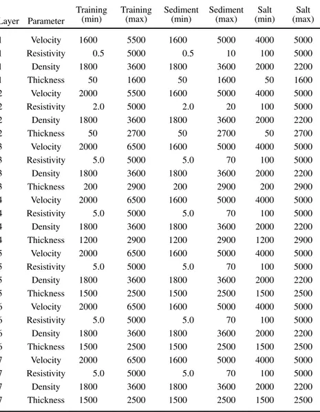
Parameter ranges.—Another important bound on the model space is our belief about the prior plausible model parameter ranges. It is implicit that the model parameterization should be chosen so as to be capable of describing the full range of prior plausible models using as few parameters as possible and also that it should be as unique as possible. Here, we consider 1D joint common structure models (Jegen-Kulcsar et al., 2009). Thus, we choose a parameterization of velocities, densities, and resistivities for a series of layers of common variable thickness. A fuller treatment would involve quantitatively trialing the ability to represent appropriate geologic formations and data sets using a range of numbers of model layers that is in itself part of the model space definition. In this case, we considered that after informal qualitative testing, models parameterized by seven layers seemed sufficient in providing the ability for the system to discern structure, particularly in the shallow region and the salt body, while not overparameterizing the system given the resolution of the observed data sets. The prior model parameter ranges for each of these layers are shown in Table 1.

Prior salt probability.—A more subtle constraint on the prior model space is the prior probability of salt existing in each layer.

For this study, we specify this to be 0.5 for each layer. In each screening cycle, for each layer, salt or sediment models are generated in the ratio appropriate to the fraction of models (the likelihood of salt present) deemed plausible for that layer from the previous cycle.

Building an emulator

Having specified the prior model space from which we intend to draw candidate models, we now construct an emulator for each of the seismic, gravity, and MT cases. We describe the process in detail for the seismic case and adopt a similar approach for the MT and gravity cases. The framework for each of these, including the full set of governing equations, is given in AppendixA. The model space used for training each emulator was simply defined by the range of parameter values considered plausible in each of the velocity, resistivity, density, and thickness cases (Table1). In other words, each

0.1 1 10 100 1000 10000 100000

1000 2000 3000 4000 5000 6000 7000

Resistivity (Ωm)

Velocity (m/s) Salt

Sediment

Sediment Salt

2 2.2 2.4 2.6 2.8 3 3.2 3.4

2000 3000 4000 5000 6000 7000

Density (kgm–3)

Velocity (m/s)

a)

b)

Figure 3. (a) Resistivity versus velocity and (b) density versus velocity relationships derived from well-log data. The borehole is located adjacent to station ST5 (Figure2). Data points were characterized by location on the plot as being from salt or sediment, and regions defined from which appropriate combinations of velocity and resistivity parameters could be drawn. The salt region was defined as a rectan- gular box, whereas the sediment relationship was defined by fitting a polynomial curve (equation5). The fitted relationship and associated uncertainty for resistivity are shown in equations5–7and the equiv- alent relations for density are given in equations8–9. The bounds shown here are for the 99% confidence bound (3σ). Data are kindly provided by Statoil.

Downloaded 03/17/16 to 129.234.252.65. Redistribution subject to SEG license or copyright; see Terms of Use at http://library.seg.org/

(7)

emulator was built independently for each modeling domain (seismic, gravity, and MT), using uniform distributions over the parameters in columns 1–4 of Table1, and without any statement about the origin of the models being used.

Seismic emulator

In constructing a seismic emulator, we use a method similar to that ofRoberts et al. (2010,2012), but here we develop and improve the results by fitting weighting coefficients to Laguerre polynomial functions rather than fitting simple polynomial functions. We choose to use Laguerre polynomials because of their mutual orthogonality, which increases the efficiency in fitting the functions concerned. Other classes of orthogonal polynomials could have been chosen here; however, Laguerre polynomials were a convenient choice. The exponential weighting associated with Laguerre polynomials means that the fitting process here may

be more sensitive to lower parameter values. In a more thorough treatment, this could be a focus for investigation; however, no significant issues were encountered here, and they were deemed fit for purpose. Depending on the setting, other functions may be more suitable to choose for the bases; if the aim was to fit to periodic data, a natural choice of basis functions would have been a Fourier series, for example. For the first cycle, we consider the velocity model space shown in Table1, parameterized by 14 parameters;ðvm; smÞ⁷_m¼1whereviandsiare the velocities and thicknesses ascribed to each of the seven layers, as shown in Table1. The model space is designed such that there is finer stratification in the shallow region. This reflects the fact that as a result of having traveltime data out to approxi- mately 10 km of offset, we expect greater seismic sensitivity in the upper 3 km or so. Our aim in building the emulator is to predict, to a calibrated uncertainty, the seismic forward code output for models drawn from this space. We generate a 1500×14Latin hypercube (McKay et al., 1979;

Stein, 1987) and use this to create a set of 1500 models over the 14-parameter space, which fill the space evenly. Each of these 1500 14-parameter models is then passed in turn to the forward seismic simulator, producing 1500 t versus x plots, each consisting of 100 (x,t) pairs. The simulator computes traveltimes using a finite element method (Podvin and Lecomte, 1991; Heincke et al., 2006). Laguerre polynomial functions are then fitted, using a least-squares algorithm, to each of these data sets (equation10) to compute a vec- tor of polynomial coefficients αx;i to represent each of thei¼1−1500data sets. It was found that Laguerre polynomials of order 3, parameterized by fourαx;i coefficients to weight the polynomials, are sufficient to recover the form of the data and keep the least-squares algorithm stable.

Our code is designed such that if a singularity oc- curs in the fitting of the coefficients (i.e., overfitting of the data is occurring), then the number of

coefficients is automatically decreased until a stable fit is achieved. In early versions of the code, simple polynomials were used as basis functions instead of Laguerre polynomials and overfitting of the data points was commonplace; however, using Laguerre polynomials, with the property of orthogonality over the space concerned, has meant that such overfitting using the number of coefficients specified here has been eliminated. Thus, we reduce each plot of 100 data points to a set of four coefficients. In using these polynomial coefficients to represent the (x,t) data, there is a misfit function that we denote asg_xðxÞ, as follows:

t¼X^p^x

i¼0

αi;xxⁱe⁻^xL_iðxÞ

þg_xðxÞ: (10)

Table 1. Prior parameter bounds for each layer. Ranges are shown for emulator training, and the ranges used to sample models from each of the sediment and salt cases. Velocity values are given in units of m∕s, resistivity values are given in units ofΩm, density values are given in units of kg∕m, and the layer thickness values are given in units of m.

Layer Parameter

Training (min)

Training (max)

Sediment (min)

Sediment (max)

Salt (min)

Salt (max)

1 Velocity 1600 5500 1600 5000 4000 5000

1 Resistivity 0.5 5000 0.5 10 100 5000

1 Density 1800 3600 1800 3600 2000 2200

1 Thickness 50 1600 50 1600 50 1600

2 Velocity 2000 5500 1600 5000 4000 5000

2 Resistivity 2.0 5000 2.0 20 100 5000

2 Density 1800 3600 1800 3600 2000 2200

2 Thickness 50 2700 50 2700 50 2700

3 Velocity 2000 6500 1600 5000 4000 5000

3 Resistivity 5.0 5000 5.0 70 100 5000

3 Density 1800 3600 1800 3600 2000 2200

3 Thickness 200 2900 200 2900 200 2900

4 Velocity 2000 6500 1600 5000 4000 5000

4 Resistivity 5.0 5000 5.0 70 100 5000

4 Density 1800 3600 1800 3600 2000 2200

4 Thickness 1200 2900 1200 2900 1200 2900

5 Velocity 2000 6500 1600 5000 4000 5000

5 Resistivity 5.0 5000 5.0 70 100 5000

5 Density 1800 3600 1800 3600 2000 2200

5 Thickness 1500 2500 1500 2500 1500 2500

6 Velocity 2000 6500 1600 5000 4000 5000

6 Resistivity 5.0 5000 5.0 70 100 5000

6 Density 1800 3600 1800 3600 2000 2200

6 Thickness 1500 2500 1500 2500 1500 2500

7 Velocity 2000 6500 1600 5000 4000 5000

7 Resistivity 5.0 5000 5.0 70 100 5000

7 Density 1800 3600 1800 3600 2000 2200

7 Thickness 1500 2500 1500 2500 1500 2500

Downloaded 03/17/16 to 129.234.252.65. Redistribution subject to SEG license or copyright; see Terms of Use at http://library.seg.org/

(8)

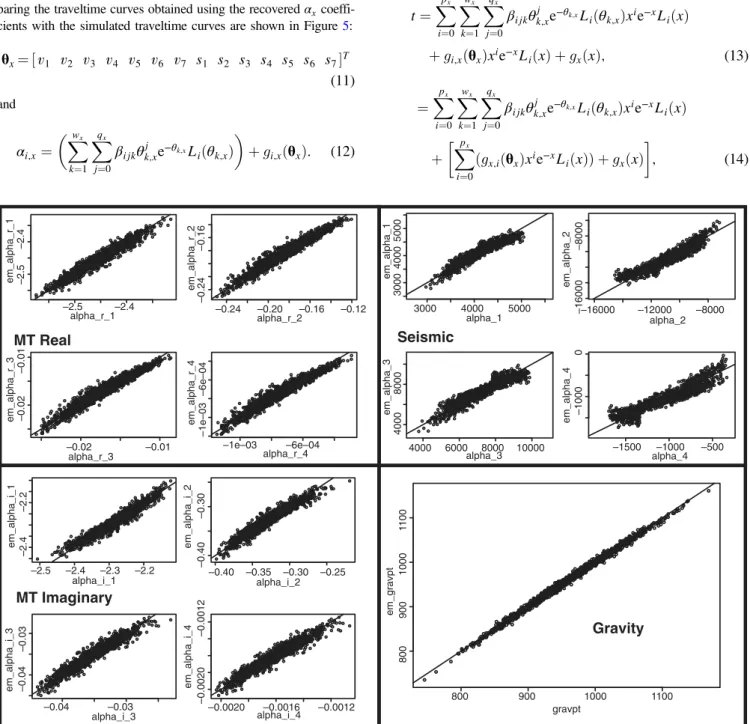
We then fitα⁴_x;i¼1to the model parameters (in this case, the velocity and layer thickness parameters½vm; sm⁷_m¼1), again using a least- squares method to fit the weighting coefficients for Laguerre polynomials. This is similarly accomplished using Laguerre polynomials up to third order in each of the layer parameters (equations11and 12). The result is a set of 228βx;ijkcoefficients (four for each of the 14 model parameters, plus a zeroth-order term, for each of the four αx;icoefficientsð¼ ð4×14þ1Þ×4Þ). Again, there is a misfit function associated with this fitting step (equation13). Examples of the recovery of theαxcoefficients using theβxcoefficients are shown in Figure4. Using theseαxcoefficients, we can then construct the traveltime curves for a given set of model parameters. Examples comparing the traveltime curves obtained using the recoveredαxcoeffi- cients with the simulated traveltime curves are shown in Figure5:

θx¼ ½v₁ v₂ v₃ v₄ v₅ v₆ v₇ s₁ s₂ s₃ s₄ s₅ s₆ s₇^T (11) and

αi;x¼X^w^x

k¼1

X^q^x

j¼0

βijkθ^jk;xe^−θ^k;xL_iðθk;xÞ

þg_i;xðθxÞ: (12)

In predicting the parametric components of the system, we have two sources of misfit in the process of building the emulator:gxðxÞ andgx;iðθxÞ, as in equations10and12, respectively. In equations12–

15, we group the terms so as to separate the parametric and nonparametric parts of the system and obtain the global misfit function Gðx;θxÞ, which is a function of offsetxand the model parameters θx. A more careful treatment of the system would involve considering this dependence. However, on the grounds of simplicity of calibration given the proof-of-concept nature of this study, we chose to compute a misfit function averaged over all model parameters. Thus, we consider the misfit functionG_xðxÞ, as shown in equations16and17:

t¼X^p^x

i¼0

X^w^x

k¼1

X^q^x

j¼0

βijkθ^jk;xe^−θ^k;xL_iðθk;xÞxⁱe⁻^xL_iðxÞ

þg_i;xðθxÞxⁱe⁻^xL_iðxÞ þg_xðxÞ; (13)

¼X^p^x

i¼0

X^w^x

k¼1

X^q^x

j¼0

βijkθ^j_k;xe^−θ^k;xL_iðθk;xÞxⁱe⁻^xL_iðxÞ

þX^p^x

i¼0

ðg_x;iðθxÞxⁱe⁻^xL_iðxÞÞ þg_xðxÞ

; (14)

Seismic

3000 4000 5000

300040005000

–16000–16000–8000 –12000 –8000

4000 6000 8000 10000

40008000

–1500 –1000 –500

–10000

alpha_4 alpha_2

em_alpha_2em_alpha_4

em_alpha_1em_alpha_3

alpha_1

alpha_3

MT Imaginary

–2.5 –2.4 –2.3 –2.2

–2.4–2.2

–0.40 –0.35 –0.30 –0.25

–0.40–0.30

–0.04 –0.03 –0.04–0.03

–0.0020 –0.0016 –0.0012

–0.0020–0.0012

alpha_i_3 em_alpha_i_3em_alpha_i_1

alpha_i_1

em_alpha_i_4em_alpha_i_2

alpha_i_4 alpha_i_2

Gravity

800 900 1000 1100

80090010001100

gravpt

em_gravpt

MT Real

–2.5 –2.4

–2.5–2.4

–0.24 –0.20 –0.16 –0.12

–0.24–0.16

–0.02 –0.01

–0.02–0.01

–1e–03 –6e–04 alpha_r_4 alpha_r_2

em_alpha_r_4em_alpha_r_2

em_alpha_r_3em_alpha_r_1

alpha_r_3 alpha_r_1

–1e–03–6e–04

Figure 4. Example reconstruction ofαcoefficients fromβcoefficients for ST12. In the case of the gravity emulator, note that we are simply representing a single point, rather than a function represented byαcoefficients, and so we plot the emulator-reconstructed points against the

“actual”points generated by the gravity simulator. Note the strong correlation between emulated and simulated outputs in each case.

Downloaded 03/17/16 to 129.234.252.65. Redistribution subject to SEG license or copyright; see Terms of Use at http://library.seg.org/

(9)

¼X^p^x

i¼0

X^w^x

k¼1

X^q^x

j¼0

βijkθ^j_k;xe^−θ^k;xL_iðθk;xÞxⁱe⁻^xL_iðxÞ þGðx;θxÞ;

(15)

≈X^p^x

i¼0

X^w^x

k¼1

X^q^x

j¼0

βijkθ^jk;xe^−θ^k;xL_iðθk;xÞxⁱe⁻^xL_iðxÞ þG_xðxÞ;

(16) and

G_xðxÞ ¼

ffiffiffiffiffiffiffiffiffiffiffiffiffiffiffiffiffiffiffiffiffiffiffiffiffiffiffiffiffiffiffiffiffiffiffiffiffiffiffiffiffiffiffiffiffiffiffiffiffiffiffiffiffiffiffiffiffiffi Pn_max

n¼1ðtem;nðxnÞ−t_sim;nðxnÞÞ² n_max

s

: (17)

To properly effect the screening of model space using a predictive simulator proxy, it is necessary to calibrate the uncertainty on the predictor. We calibrate the emulator uncertainty in usingβxfor prediction by computingGxðxÞ, as in equationA-8. This is done by generating theβx-coefficient estimated output function and the full simulator output for each training model parameter set (Figure5) and computing the root mean square (rms) of the residuals with respect to the traveltime functions used to train the emulator as a function of x. Examples of this misfit function are shown in Figures6a–9a.

A key question is,“How many training models are required to correctly estimate G_xðxÞ and thus sufficiently sample the model space?”This question is vitally important for two reasons: first, because a model’s plausibility or implausibility can only be reliably determined if the emulator uncertainty with respect to the estimation of the simulator output is correct and second because the aim at each screening cycle is to exclude model space not deemed plausible; it is crucial to properly sample the whole of the remaining space to pre- vent the model space from being wrongly removed. If the model coverage is not sufficient, then the emulator will underestimate the predictive uncertainty. A more rigorous study would involve either a more detailed assessment of the space to be sampled or the inclusion in the sampling method of a finite probability of sampling outside the currently constrained space. Using the criterion of two samples/

parameter, we would wish to use2¹⁴≈16000training models (for example, as inSambridge and Mosegaard, 2002). For our purposes, we chose a semiqualitative and fairly rudimentary approach of considering that if the coverage is sufficient, then the addition of further model parameter sets to the training process will not significantly alter the uncertainty estimate. We therefore calibrated the number of models needed by testing cases of generating the emulator using 150, 1500, and 15,000 training models and assessing the impact on the emulator uncertainty of adding more models to the training process. For emulators trained over our prior model space (Table1), it was found that using 150 models was insufficient (Figure5), but that the uncertainty function estimates using 1500 and 15,000 training models give similar uncertainty functions. Over this space, therefore, 1500 models is deemed a sufficient number with which to train the emulator.

The set of βx coefficients and this uncertainty functionG_xðxÞ togetherconstitute the emulator, or statistical model. We use this

uncertainty function to determine whether emulated output data of a proposed model lie sufficiently close to the observed data sets such that the model can be deemed plausible or not. However, G_xðxÞis calculated as the rms of the simulator-predictor residual, and as such it is possible (and indeed, it is certainly the case in some instances) that the actual data-representation error for a given set of model parameters may be significantly larger than this. Hence, it may be the case that potentially plausible models are rejected by the emulator screening simply because the emulator prediction for that set of model parameters was located in the tail of the uncertainty function. The emulator screening reliability is, therefore, tested by using this screening technique on 100 target data sets, produced by the simulator from 100 synthetic models. A scaling factorγxfor the uncertainty function is then calculated by calibrating against these 100 target data sets, such that there is at least a 97% probability that the emulator screening process will include the“true”model in its selection of plausible models if the true model is included in the candidate model space. The figure of 97% is in many senses arbitrary; however, we considered it suitable for the purpose at hand.

The condition for plausibility is shown in equation 18, where

2 4 6 8 10

0 2

Offset (km)

Time(s)

4

2 4 6 8 10

Offset (km)

Time(s)

2 4 6 8 10

Time(s)

2 4 6 8 10

Time(s)

0 50 100 150 200 250 300

1 2 3 4 5 6 7 8 9 10

Travel time residual (ms)

Offset (km) 15000 runs

1500 runs 150 runs 0

2 4

0 2 4

Offset (km) Offset (km)

a)

b)

Figure 5. (a) Four example traveltime training outputs and emulator- reconstructed outputs. Black ovals show the traveltimes generated by the full simulator code, and the gray lines show the traveltime curves predicted by applying the predictiveβcoefficients to the same sets of model parameters. (b) Comparison of seismic emulator uncertainty function for ST13 after eight cycles using 15,000, 1500, and 150 training models.

Downloaded 03/17/16 to 129.234.252.65. Redistribution subject to SEG license or copyright; see Terms of Use at http://library.seg.org/

(10)

temðxnÞandttargðxnÞare the emulated and full simulator traveltimes at an offset xn, respectively. The weights κx;n are user-defined weights for each traveltime point. For example, we attach greater importance to achieving a close fit to the short-offset traveltimes, compared with the long-offset measurements on the basis that the velocity gradient is typically higher in the shallow structure. Table4 shows the values ofκused in this study. Here, we have chosen to give all points a weighting of either 1 or 0, and varied the density of points along the offset profile with value 1 to control the weight given to varying parts of the traveltime curves. If preferred, the user could easily use fractional weights:

Xⁿ^max

n¼1

κx;n

max½jðt_emðx_iÞ−t_targðx_iÞÞj−γxG_xðx_iÞ;0 G_xðxnÞPn_max

p¼1κx;p

<n_max:

(18)

Spike emulator

To locate discontinuities in the gradient of the seismic traveltime curves and thus constrain abrupt changes in velocity at layer boundaries, a“spike”emulator was built. There are a number of other approaches (Grady and Polimeni, 2010), which could have been taken to identify the boundary positions, such as the basic energy

0.35 0.30 0.25 0.20 0.15 0.10 0.05 0.00

MTemulatoruncertainty

–2.0

–3.0 –1.0

log (frequency)10

–2.0

–3.0 –1.0

log (frequency)10

0.35 0.30 0.25 0.20 0.15 0.10 0.05 0.00

MT Re(Z) MT Im(Z)

30 25 20 15 10 5 0

Gravityemulatormisfit(mGal)

20 15 10 5 0

Cycle number

20

15

10

5

0 Spikeemulatoruncertaintyin datapointnumber

3 2

1

Spike number 25

Spike Gravity

Offset (km)

Seismic

350 300 250 200 150 100 50 0 Seismicemulator uncertainty(ms)

4 6 8

2 10

Uncertainty reduces with increasing cycle number

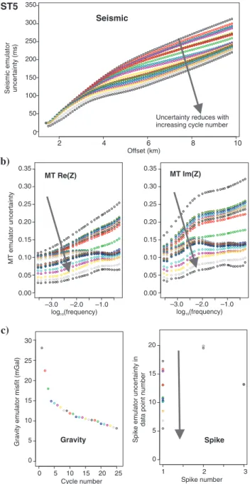
ST5 a)

b)

c)

Figure 6. (a) Seismic, (b) MT, and (c) gravity uncertainty functions for ST5. Arrows show how the predictive uncertainty of the emulators reduce with the increasing screening cycle as the model space is refined.

Offset (km)

30 25 20 15 10 5 0

Gravity emulator misfit (mGal)

20 15 10 5 0

Cycle number

20

15

10

5

3 2

1

Spike number 25

Gravity Spike

Seismic

4 6 8 1

2 0

ST7 a)

b)

c)

0.35 0.30 0.25 0.20 0.15 0.10 0.05 0.00

–2.0

–3.0 –1.0

log (frequency)10

–2.0

–3.0 –1.0

log (frequency)10

0.35 0.30 0.25 0.20 0.15 0.10 0.05 0.00

MT Im(Z) MT Re(Z)

Figure 7. (a) Seismic, (b) MT, and (c) gravity uncertainty functions for ST7. Arrows show how the predictive uncertainty of the emulators reduce with increasing screening cycle as the model space is refined.

Downloaded 03/17/16 to 129.234.252.65. Redistribution subject to SEG license or copyright; see Terms of Use at http://library.seg.org/

(11)

model and the total variation model. Each has strengths and weak- nesses, particularly regarding how noise is regarded in association with high-frequency data. A key part of the philosophy of our method is that it should be as conceptually straightforward as possible and data driven wherever appropriate, and so we chose to implement the simple gradient detection method, described here. In building the seismic emulator, the chosen form of data reduction of using polynomial curves to represent thetversusxcurves, while being suitable for describing the smooth trends (Figure5), does not capture discontinuities in the traveltime gradient functiondt∕dx.Rob- erts et al. (2012) describe a strategy to consider these gradient

discontinuities, whereby the dependence of the offset position of these gradient discontinuities is considered as a function of the seismic model parameters. We adopt the same strategy here, seeking to model such features in the data, and thus capture structural information, with a view to optimizing the positions of the model layer boundaries, thus best representing the substructure.

As inRoberts et al., (2012), instead of consideringdt∕dxto probe this information, we calculate the squared second derivative of thet versusxfunctionψ¼ ðd²t∕dx²Þ²(Figure10). In principle, given that we are using seven-layer models, to optimize the layer boundary positions, we could search for the six largest spikes. However, the presence of six discernible spikes in many of the observed seismic CMP gathers is unlikely (see Figure2for example), and this may yield the positions of noise spikes (the positions of which would likely be uncorrelated to any structural information). To avoid potential computational problems as a result of misattributing structurally sourced gradient discontinuities to noise, we choose to only estimate the offset positionsxof the three largest spikes in this ψ¼ ðd²t∕dx²Þ²function. We preferentially useðd²t∕dx²Þ² as opposed tod²t∕dx²to ensure thatψis positive, simplifying the process of picking the extrema, in addition to exaggerating the relative magnitudes of the spikes in question. A key assumption of this method is that the largest spikes do represent layer boundaries, rather than noise. For cases in which there is a high degree of noise, it may be necessary to either consider other methods for the detection of structural boundaries or reduce the number of model layers and the expected output resolution.

For each seismic emulator training data set, we therefore compute (numerically) ψ¼ ðd²t∕dx²Þ² and then search for the offset x

Offset (km)

0 2 4 6 8 10 12

0 2000 4000 6000 8000 10000

140 220

100 60 20 Emulator uncertainty (ms) Distance (m)

0.02 0.06 0

–0.5 –1.0 –1.5 –2.0 –2.5 –3.0 –3.5

log (frequency)

0.12 0.08 0

–0.5 –1.0 –1.5 –2.0 –2.5 –3.0 –3.5

log (frequency)

Seismic emulator uncertainty

(Uncertainty in ability to predict travel time data)

MT emulator uncertainty (Uncertainty in ability to predict Re(Z))

R

MT emulator uncertainty (Uncertainty in ability to predict Im(Z))

I

0.10 Emulator uncertainty

Emulator uncertainty

0.04 0.16 180

0.18 0.14

0.20 0.24

c) b) a)

ST1 ST2 ST3 ST4 ST5 ST6 ST7 ST8 ST9 ST10 ST11 ST12 ST13 ST14 ST1 ST2 ST3 ST4 ST5 ST6 ST7 ST8 ST9 ST10 ST11 ST12 ST13 ST14 ST1 ST2 ST3 ST4 ST5 ST6 ST7 ST8 ST9 ST10 ST11 ST12 ST13 ST14

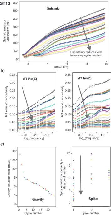
Figure 9. (a) Seismic and (b-c) MT emulator uncertainty functions (GxðxÞandG_ωðωÞ) for each station. These data maps represent the predictive uncertainty of the emulator in predicting the simulator output. White lines show the positions of the stations between which the function is interpolated.

0.35 0.30 0.25 0.20 0.15 0.10 0.05 0.00

–2.0

–3.0 –1.0

log (frequency)10

–2.0

–3.0 –1.0

log (frequency)10

MT Re(Z) MT Im(Z)

0.35 0.30 0.25 0.20 0.15 0.10 0.05 0.00

30 25 20 15 10 5 0

Gravityemulatormisfit(mGal)

20 15 10 5 0

Cycle number

20

15

10

5

3 2

1

Spike number

Gravity Spike

4 6 8

2 10

Offset (km) Seismic

ST13 a)

b)

c)

Figure 8. (a) Seismic, (b) MT, and (c) gravity uncertainty functions for ST13. Arrows show how the predictive uncertainty of the emulators reduce with increasing screening cycle as the model space is refined.