Research Collection
Monograph
Invitation to Quantum Informatics
Author(s):
Aeschbacher, Ulla; Hansen, Arne; Wolf, Stefan Publication Date:
2020-01-28 Permanent Link:
https://doi.org/10.3929/ethz-b-000395060
Originally published in:
http://doi.org/10.3218/3989-4
Rights / License:
In Copyright - Non-Commercial Use Permitted
This page was generated automatically upon download from the ETH Zurich Research Collection. For more information please consult the Terms of use.
and its processing on the one hand, and physics on the other.
In the spirit of Rolf Landauer’s slogan „Information is physical,“
consequences of physical laws for communication and compu- tation are discussed, e.g. the second law of thermodynamics.
In the second part, the pessimism of the first part is overcome and new possibilities offered by the laws of quantum physics for infor- mation processing are discussed:
cryptography, teleportation, dense coding, and algorithms such as Grover’s. The culmination point is Shor’s miraculous method for efficiently factoring integers.
The epilogue is an extended version of the third author’s closing lecture of the seminar
„Information & Physics (& Science Sociology),“ in which Landauer’s sentence is contrasted with John Archibald Wheeler’s „It from Bit.“
www.vdf.ethz.ch
In vi ta ti on t o Q u an tu m I n fo rm at ic s
Aeschbacher · Hansen · WolfUlla Aeschbacher · Arne Hansen · Stefan Wolf
Invitation to Quantum
Informatics
Weitere aktuelle vdf-Publikationen finden Sie in unserem Webshop:
vdf.ch
Gerne informieren wir Sie regelmässig per E-Mail über unsere Neuerscheinungen.
› Bauwesen
› Naturwissenschaften, Umwelt und Technik › Informatik, Wirtschafts-
informatik und Mathe matik
› Wirtschaft
› Geistes- und Sozialwissen- schaften, Inter disziplinäres, Militärwissenschaft,
Politik, Recht
Newsletter abonnieren
Anmeldung auf vdf.ch
Ulla Aeschbacher · Arne Hansen · Stefan Wolf
Invitation to Quantum Informatics
Weitere aktuelle vdf-Publikationen finden Sie in unserem Webshop:
vdf.ch
Gerne informieren wir Sie regelmässig per E-Mail über unsere Neuerscheinungen.
› Bauwesen
› Naturwissenschaften, Umwelt und Technik › Informatik, Wirtschafts-
informatik und Mathe matik
› Wirtschaft
› Geistes- und Sozialwissen- schaften, Inter disziplinäres, Militärwissenschaft,
Politik, Recht
Newsletter abonnieren
Anmeldung auf vdf.ch
http://dnb.dnb.de.
All rights reserved. Nothing from this publication may be reproduced, stored in computerised systems or published in any form or in any manner, including electronic, mechanical, reprographic or photographic, without prior written permission from the publisher.
© 2020, vdf Hochschulverlag AG an der ETH Zürich ISBN 978-3-7281-3988-7 (Printausgabe)
Download open access:
ISBN 978-3-7281-3989-4 / DOI 10.3218/3989-4
www.vdf.ethz.ch
1 What Is Quantum Informatics? 5
1.1 Information & Physics . . . 5
1.2 The Stern/Gerlach Experiment . . . 7
1.2.1 Independent Measurements? . . . 7
1.2.2 Superposition . . . 9
1.3 Quantum Key Distribution . . . 10
1.4 The Double-Slit Experiment . . . 11
1.4.1 The Mach/Zehnder Interferometer . . . 12
1.5 The Quantum Bit . . . 14
1.6 Deutsch’s Algorithm . . . 15
1.7 The Aspect/Gisin/Zeilinger Experiments . . . 17
2 Information Is Physical 23 2.1 Thermodynamics and Entropy . . . 24
2.2 Information Theory . . . 26
2.2.1 Standard Model of Communication . . . 26
2.2.2 The Game of 20 Questions . . . 27
2.2.3 Connection to Probability Theory . . . 28
2.3 The Converse of Landauer’s Principle . . . 33
2.4 Bennett’s Solution to the Problem of Maxwell’s Demon . . . . 34
2.5 Reversible Computing . . . 35
2.6 The Toffoli Gate . . . 38
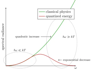
3 Key Experiments and Postulates of Quantum Physics 43 3.1 Black-Body Radiation . . . 43
3.2 Photoelectric Effect . . . 44
3.3 Wave-Particle Dualism . . . 46
3.4 Observables . . . 48
3.5 Postulates of Quantum Theory . . . 50
3.5.1 The State . . . 50
3.5.2 The Time Evolution . . . 51
3.5.3 Observables . . . 51
3.5.4 Joint Systems and Composition . . . 52
3.5.5 Abstraction and Simplification . . . 53
3.5.6 Density Matrices . . . 55
3.6 Qbits . . . 58
3.6.1 One Qbit . . . 58
3.6.2 Two Qbits . . . 59
3.6.3 The CNOT Gate . . . 64
3.6.4 Cloning, Pseudo-Cloning, and Pseudo-Measurements . . 67
4 Quantum Communication 71 4.1 Teleportation . . . 71
4.2 Superdense Coding . . . 74
5 Simple Algorithms 75 5.1 nQbits . . . 75
5.2 The Secret Mask . . . 76
5.3 The Deutsch/Josza Algorithm . . . 79
6 Pseudo-Telepathy 83 7 The Needle in the Haystack: Grover’s Algorithm 87 7.1 Motivation . . . 87
7.2 The Elements . . . 88
7.3 The Grover Circuit . . . 88
8 Integer Factoring: Shor’s Algorithm 91 8.1 Quantum Fourier Transform . . . 91
8.2 Phase Estimation . . . 93
8.3 Factoring . . . 94
9 Epilogue: Information & Physics 97
10 Bibliography 117
What Is Quantum Informatics?
1.1 Information & Physics
Physics and Information (Theory) are two different sciences,i.e., two think- ing traditions both rooted in their respective histories, coined by their own methods, personalities, and established truths. The present text belongs to the (postmodern) tradition of considering, establishing, discussing, and ana- lyzing the connections between physics and information. Of these connections, there are essentially two natures: On the one hand, experience, observation, and physical discourse are in the form of information: John Archibald Wheeler compressed this fact to the slogan “It from Bit.” On the other hand, infor- mation representation, processing, and transmission are, ultimately, physical processes; asRolf Landauer put it: “Information is Physical.”
Information Theory (Shannon)
Quantum Theory, Thermodynamics, Relativity
Landauer(1961): “Information is physical”
Wheeler(1983): “It from bit”
This text starts from the latter insight and discusses consequences thereof both of limiting (thermodynamics) and enabling (quantum theory) character of physical law for information treatment. On occasion, a glimpse is offered at the possibility of obtaining new insights into natural law when the informational point of view is chosen. The text culminates inPeter Shor’s algorithm, born out of a surprising and breathtaking marriage between quantum physics and number theory. (Claus Hepp called the algorithm the “most fascinating result in theoretical physics of its decade,” due to its internal conceptual beauty,
not its “real-world” application that is, at this point, potential, unclear, and debated.)
Concretely, Landauer’s slogan means that the representation of a bit of information, if this bit is to “exist,” must be physical. This implementation can be realized by a switch, a current in a metal wire going one way as opposed to the other, the position of a single gas molecule in a container, the polarization of a photon, or by the electron of a hydrogen atom in its ground as opposed to first excited state. The latter example is interesting since it illustrates that digitalization in fact comes very naturally with quantization (e.g., of energy levels) whereas in classical physics, it has to be enforced in some way. Later in the text, however, we will see that quantum physics allows for another kind of
“world between zero and one” that could more accurately be enabled by the possibility of “being zero and one at the same time (at least to some extent).”
If we follow that thought through, we realize that physical laws thus can have direct consequences for information processing. Although that is true in principle, it seems that the nature of these consequences probably depends strongly on the specific choice of the information’s physical representation. Or
— to turn that thought around — are those physical laws that have conse- quences that areindependentof that representation (beyond the fact that there is such a representation) perhaps laws that are rather logical-informational than “physical” in the strict sense?
The second law of thermodynamicsstates that, in a closed system,entropy does not decrease (with overwhelming probability). What is entropy? A first, rough answer is that it is some kind of measure fordisorder. A precise answer is harder; John von Neumann was quoted as saying “if you want to win any discussion, just say ‘entropy’ and you will be on the safe side, because nobody really knows what entropy is.” It has also been said thatClaude Shannon, the founder of information theory, followed von Neumann’s advice when he chose the name “entropy” for the central quantity of his theory.
A remarkable feature of the second law is itstime asymmetry, which con- trasts the time symmetry of most physical laws and processes. Exceptions are some elementary-particle reactions and, more importantly for us, measure- ments. Related notions thus would bepast andfuture: the arrow of time.
Whereas entropy (disorder) may be hard to define in general, it is clear in some cases: Given that N binary memory cells contain a “random” content (an equally problematic notion, in fact) and are then all erased (put to 0), the entropy in the set of memory cells drops.
1.2 The Stern/Gerlach Experiment
1.2.1 Independent Measurements?
The Stern/Gerlach experiment — proposed by Otto Stern in 1921 [16] and carried out by Walther Gerlach in 1922 [8] — was not the first in the his- tory of quantum theory, but one of the most important ones to understand the structure and properties of the basic building block of quantum informa- tion processing, thequantum bit (Qbit). In particular, the question was what classical information we can get on such a Qbit, and how.
In the experiment, Stern and Gerlach measure a certain quantity, themag- netic dipole moment, of silver atoms by sending a stream of such atoms, exiting an oven, through a inhomogeneous magnetic field. Each atom is then deflected from the path proportionally to its dipole in the direction of the magnets. If we imagine that the moments of the atoms point in random directions (and have, perhaps, constant length or even varying length within some range or according to some distribution), then the classical expectation is that the de- flection pattern reaches a maximum in the middle (no deflection) and then symmetrically, monotonically, and continuously decreases on the sides. This is, however, not what was observed: There is no detection in (not even close to) the middle, but rather two sharp peaks at equal distances from that middle.
N S
This “quantization” is one of the characteristic features of quantum theory — to which it owes its name, too — and motivated assigning the quantity a new name in that context: spin.1
1The following anecdote was reported concerning this experiment: Initially, Gerlach did not see any detection of the screen supposed to register the trajectories of the silver atoms.
Desperately, he handed the blind plates to Stern, who gave it a look to; during that, some of the air Stern was breathing out hit the plates. The thing is that the cigars Stern used to smoke (heavily) contained a lot of sulfur; they were cheap cigars, as physics researchers were not well paid at the time, it seems. In the end, the sulfur initiated the reaction necessary to see the detections on the screen, and the experiment succeeded. The story is sometimes taken to support the argument that also social and economic factors (Stern’s salary and the quality of his cigars, etc.) have to be considered in the context of physical experiments dismantling “objective” reality.
In the case of a single Stern/Gerlach measurement, say, in theZ-direction, two identical rays result. Let us call the rays by the properties they correspond to, i.e.,Z−andZ+.
Z
+z 50%
−z 50%
If the same measurement is repeated on, say, only the Z+ ray, then all atoms are again deflected in the + direction. In this sense, theZ-spin property looks classical: It is stable with respect to repeated measurements.
Z
+z 50%
Z
−z 50%
+z 100%
−z 0%
When the magnet is rotated into the spatialXdirection (also perpendicular to the flying directionY of the atoms), then a 50−50 distribution arises. This is not surprising due to the geometrical symmetry of the situation. It is equally unsurprising that the same is observed when the second measurement (the one inX direction) is carried outafter aZ measurement from which only the Z+ counts are carried over to the next experiments: It means that the two properties, “Z-spin” and “X-spin,” lookindependent.
Z
z+ 50%
X z− 50%
+x 50%
−x 50%
The most fascinating outcome results when the two types of measurement are combined as follows: First, aZ measurement, whereby onlyZ+ counts are transferred to the next magnet, anXmeasurement. If subsequently, anotherZ measurement is performed, then half the particles showZ−spin, although we took onlyZ+ states after the first measurement. This is puzzling and questions both our interpretations above: The stability as well as the independence of the properties in question.
Z
z+ 50%
X z− 50%
x+ 50%
Z x− 50%
z+
50%
z− 50%
Interlude
The stability of a measurement result is not so surprising: Popper re- gards scientifically interesting physical effects to be defined by being re- producible by anyone and at anytime, provided that one builds the same experimental setup.a The “scientific method” crucially relies on being able to enquire about equivalent questions and then expect the same answer.
There must at least exist some conditions under which this is possible.
This does, however, not imply that this is possible under all conditions as one might hope coming from classical mechanics.
a“Der wissenschaftlich belangvolle physikalische Effekt kann ja geradezu dadurch definiert werden, daß er sich regelm¨aßig und von jedem reproduzieren l¨aßt, der die Versuchsanordnung nach Vorschrift aufbaut.” [14,§I.8]
1.2.2 Superposition
The statistics found within the Stern/Gerlach experiment were surprising for single particles. They would not have been surprising if we had dealt with waves. Imagine a polarizing filter in a beam of light. Then measuring z+
can be considered to correspond to passing a polarizing filter of a certain orientation; measuringz− corresponds to passing a polarizing filter rotated by 90◦. If the beam initially is unpolarized, then the probability of passing such a polarizing filter—or the ratio of the intensity before and after the filter—is 50%. Measuring with a filter rotated by 45◦with respect to thez+filter would correspond tox+. Then the intensities measured in a sequence of filter would fit the probabilities in the Stern/Gerlach experiment.
The essential property of waves is that they can be linearly combined.
Quantum mechanical states have the same property: They are elements in a vector space. But their length does not relate to wave amplitudes; instead, they serve to derive probability distributions. Thus, linearly combined states have to be normalized. Thez+ filter then corresponds to asking whether the silver atom is in a z+ state, denoted by |z+. If the silver atom does not go up, i.e., it is not in a state |z+, then it goes down, i.e., it is in a state
|z−, orthogonal to |z−. So, the question whether the silver atom is in the state |z+and the question whether the silver atom is in the state |z− are complementary to one another. In fact, they can also be regarded as two different answers to the same question, i.e., theZ measurement.
If, after aZ measurement, we perform anX measurement, then we want to know whether the silver atom is in a state|x+or in a state|x−. Both are equal superpositions,
|x+= 1
√2|z++ 1
√2|z− |x−= 1
√2|z+ − 1
√2|z−.
No matter whether we had obtained z+ or z− in the Z measurement, the X measurement yields one of both results with equal probability.2 Also in the inverse order: A Z measurement after an X measurement yields the same uniform distribution—independent of any measurements before the X mea- surement.
|z+
|z−
|x+
|x− 45◦ 45◦
Interlude
So, a phenomenological perspective, i.e., from a comparison of probability distributions, suggests the superposition of states in quantum mechanics.
Quantum mechanics attains an essential property of wave mechanics, even though there are no more coupled system, with a description in, e.g., classical mechanics. The states are then more abstracts entities. They are no longer directly observable properties of a system, but rather tools to determine probability distributions for measurement results.a
aGrete Hermanndescribes quantum states as “new symbols that express the mutual dependency of the determinability of different measurements.” [10]
1.3 Quantum Key Distribution
Previously we have seen: The condition for measuringwith certainty the same value in two consecutive measurements with the same measurement basis, e.g., in two consecutive Z measurements, is that there is no intermediary measurement in another bases. In other words: The interactions of a system with its environment, within, say, a measurement, become traceable. This allows us to detect an eavesdropper in a cryptographic key agreement protocol.
In 1984, Gilles Brassard and Charles Bennett developed the first application of quantum mechanics for cryptographic purposes with such a key agreement protocol [2].
Let us assume that Eve and Bob can exchange quantum mechanical sys- tems. Then they can establish a secret key as follows: Alice chooses at random
2The details of how to derive probabilities from states will be given later.
a measurement, eitherZ or X, and measures a quantum system, e.g., a silver atom, in that basis. She then sends that system to Bob, who also chooses at random between aZ and anX measurement, and performs the measurement on that system. If the bases that Alice and Bob choose co¨ıncide, then the results of their measurements are the same—unless there has been an eaves- dropper, Eve, measuring the system during its transmission from Alice to Bob in a basis different from Alice’s and Bob’s. Alice and Bob do not agree be- forehand on a basis. Instead, they repeatedly measure quantum systems in randomly chosen bases. So, Eve can merely guess Alice’s choice of measure- ment. If Alice’s choice was really random then, in some cases, Eve guesses wrongly and, therefore, disturbs the system. Alice and Bob can trace that dis- turbance as follows: Alice repeatedly chooses random measurement and sends the states after the measurement over to Bob, e.g.,
Alice’s measurement × + + × + × × + ×
result 0 0 1 0 1 1 0 0 1 .
Bob also chooses his bases at random and measures the state:
Alice’s measurement × + + × + × × + ×
result 0 0 1 0 1 1 0 0 1
Bob’s measurement + + + + × × + + +
result 1 0 1 0 0 1 1 0 1
.
Where their bases agree, their measurement result are the same, if there is no eavesdropper. So, Alice and Bob communicate over an authenticated channel the positions in the above sequence where they do agree. Now, to ensure that there has been no eavesdropper, they finally choose randomly some of the positions where their results should be the same and compare whether they actually are. If Eve had been intercepting and measuring the states, then the results should differ in about 1/4 of the cases. If Alice and Bob find that their results are the same in (almost) all cases, then they can use the remaining, unpublished measurement result (where their measurement bases agree) as a secret key.
1.4 The Double-Slit Experiment
If one shines light onto a double slit, an interference pattern appears on a screen behind the double slit. What happens, however, if one sends single electrons orsingle photons onto the double slit? Intuitively one would expect two peaks, corresponding to each of the slits. Instead, if one measures the position of the electrons or photons on the screen for many repetitions of the experiment, an interference pattern emerges.
expected distribution measured interfer- ence pattern
Surprisingly, single particles exhibit wave properties. In a sense, the differ- ent paths the particle could have taken interfere with one another. If one measures, however, which path the particle has taken, then the interference pattern vanishes.
1.4.1 The Mach/Zehnder Interferometer
The Mach/Zehnder interferometer can be considered a variant of the double- slit experiment. If one sends single photons into a Mach-Zehnder interfero- meter
D1
D2
then interference occurs, and the photon is detected with certainty in detec- torD1. More precisely: In each reflection, the state of the photon picks up a phase shift ofπ/2. If we label the state of a photon moving to the right by|1 and a photon moving up by |2, then the effect of the fully-reflecting mirrors is
|1 →i|2 |2 →i|1, and the effect of the semitransparent mirrors is
|1 → 1
√2(|1+i|2) |2 → 1
√2(|2+i|2) .
This characterizes two linear maps that allow tracing the state of photon as it moves through the interferometer after its emission from the source
|1 → 1
√2(|1+i|2)→ 1
√2(i|2 − |1)
→ 1
√2 1
√2(i|2 − |1)− 1
√2(|1+i|2)
=−|1.
With a probability of 1/2, the photon passes the semitransparent mirror with- out being affected, and with the same probability it is reflected and picks up a phase shift ofπ/2. So after the second semitransparent mirror, the photon is in a state−|1, and will be measured with certainty in detectorD1.3
If, however, one measures whether the photon has gone through the upper or the lower arm of the interferometer, then the state before the last semitrans- parent mirror iseither |1or |2. In that semitransparent mirror the state of the photon is then mapped to either 1/√
2(|1+i|2) or 1/√
2(|2+i|1). In both cases the photon is detected in either of the detectors with equal probabil- ity. Thus, a measurement about the path of the photon affects the interference.
This effect can be used to detect explosive bombs.
Interlude: Interaction-free measurements
In 1993, Avshalom Elitzur and Lev Vaidman [7] proposed a method for measuring without interacting, employing a Mach/Zehnder interferometer in the following way. Imagine a bomb that is triggered by a single photon.
How could one detect such a bomb? Looking at it would expose it to photons and thus explode it. There is a way around it. Literally. If one puts the bomb into one arm of a Mach-Zehnder interferometer, then one can detect a photon if it travels through theother arm.
D1
D2
The bomb measures which path the photon has taken and thus affects the interference: The photon can now be measured in the detector D2
with probability 1/4, where, without the bomb, it would not have been measured at all. If, in the first measurement, the photon was detected inD1, we can simply send another photon. Then the probability to detect the photon inD2without exploding the bomb is 1/4 + 1/42. Proceeding
3The minus sign is irrelevant for the probability distribution, as we will see later in the course.
this way, we can reach a probability of ∞
n=1
1/4n= 1/4 ∞ n=0
1/4n= 1/3.
But the bomb still explodes with probability 1/2. How could we reduce this threat? For instance, we could encapsulate the multiple interferome- ter:
Another equivalent way of reducing the threat of explosion is to make the first semitransparent mirror almostintransparent and the second almost transparent.
1.5 The Quantum Bit
To transfer a bitb∈ {0,1}into the quantum world, we associate 0 and 1 with two orthogonal vectors, usually with the standard basis vectors,
|0= 1
0
|1= 0
1
A general quantum state can then be written as a superposition|ψ=α|0+ β|1, withα, β∈Cand|α|2+|β|2= 1. Measuring |ψin the standard basis yields 0 with probability |α|2 and 1 with probability |β|2. Quantum circuits are composed of quantum gates, i.e., unitary maps. The most important of these is the Hadamard gate,
H = 1
√2
1 1 1 −1
which maps the basis states to superpositions, H|0= 1
√2(|0+|1) H|1= 1
√2(|0 − |1). Applying the Hadamard gate again, yields the standard basis vectors.
Another interesting gate is F = 1
√2i
1 i i 1
because applying the gates twice, yields the not-gate, F·F =
0 1 1 0
.
Classically there is no gate that yields the not-gate this way: F has been called the “square root of NOT,”
F =√ NOT.
1.6 Deutsch’s Algorithm
Interference is an essential ingredient in Deutsch’s algorithm. Let us assume we are given a black box that implements a function
f :{0,1} → {0,1}.
The question is: Isf constant or not? Isf(0)⊕f(1) zero or one? Classically, we have to query the black box twice to find out. But we can do better with the help of quantum mechanics. To achieve that we first have to turn the black box into a quantum black box. Because of the unitarity of the quantum mechanical time evolution, the quantum version has to be reversible. Thus, we assume that the quantum black box implementingf is a gate of the form
|x |x
|a |f(x)⊕a
So if a is 0, then x is mapped to |f(x) on the output wire. And if a is 1, then xis mapped to |f(x), where the overline indicates the negation. The box characterizes a map by linear extension. A first idea might be to put a superposition on the input wire and setato 0. We have to consider both input wires together4 and obtain the combined input
√1
2(|0+|1))⊗ |0
= 1
√2(|0 ⊗ |0+|1 ⊗ |0)).
4See Section 3.5 for tensor products describing combined systems.
The first summand is mapped to |0 ⊕ |f(0) and the second to|1 ⊕ |f(1). Linearly combining the two we obtain
√1
2(|0+|1))⊗ |0 → 1
√2(|0 ⊕ |f(0)+|1 ⊕ |f(1))) .
The resulting state is entangled, and we cannot access the information about f(0) andf(1) by merely measuring the output wire.
The magic happens when we put a superposition on the second wire as well. If we set|a= 1/√
2 (|0 − |1), then we can expand the combined input as
√1
2(|0+|1)⊗ 1
√2(|0 − |1)
= 1 2
|0 ⊗ |0 − |0 ⊗ |1+|1 ⊗ |0 − |1 ⊗ |1 .
Applying the gate to each of the summands and linearly combining the result yields
√1
2(|0+|1))⊗ 1
√2(|0 − |1))
→ 1
2
|0 ⊗ |f(0) − |0 ⊗ |f(0)+|1 ⊗ |f(1) − |1 ⊗ |f(1)
= 1 2
|0 ⊗
|f(0) − |f(0)
+|1 ⊗
|f(1) − |f(1)
So, iff(0) =f(1), then the last line is equal to 1
2(|0+|1)⊗
|f(0) − |f(0)
; otherwise
±1
2(|0 − |1)⊗
|f(0) − |f(0) .
Then, measuring in the standard basis after applying a Hadamard gate yields 0 if the first is the case and 1 if the latter is the case.
1/√
2(|0+|1) H M
1/√
2(|0 − |1)
0 iff is constant
1 iff is not constant
Deutsch’s algorithm does not allow us to retrievemore information. The last measurement still just returns one bit. It yields the actual value of neither f(0) nor of f(1). Rather, the algorithm allows accessing the right bit, i.e., f(0)⊕f(1).
1.7 The Aspect/Gisin/Zeilinger Experiments
The power of quantum computing and quantum information processing lies in the fact that a pair of Qbits is more than “one Qbit plus another Qbit.” A particularly striking manifestation of that additional quality is revealed in the correlations that arise when two Qbits which are in a so-calledentangled state are independently measured.
Imagine that, in a preparation central, pairs of Qbits (e.g., polarized pho- tons) are generated and sent onto their respective paths to two parties, Alice and Bob. They measure the particles, for instance, both in the standard basis, and observe (when they compare their data) certain correlations, for instance, the same bit in every run.
source MB
MA
Assume for the sake of the argument that this is exactly what they see:
The same bit in every run. Is this surprising? Is there something mysterious about it? A priori not at all: We are surrounded by correlations, and we are often interested in how they arose. Let us give it a try in the given situation:
One possibility is that, in the preparation center, a coin in flipped in each run, and according to the outcome either a QBit in state|0is sent to both parties (we call this state|0 ⊗ |0, where for the moment, the symbol⊗is simply to be read as “and:” Alice receives|0andBob receives|0), or|1to both (i.e., state|1 ⊗ |1). When they then measure the respective particles, they have their perfect correlation. But this is not how it was done in these experiments;
it would also not have been very interesting, by the way.
Whatwas actually sent and measured are the two parts of theequal super- positionof the above two states and not their “classical-probabilistic” mixture:
|0 ⊗ |0+|1 ⊗ |1
√2 .
Since the probability amplitudes of the two basis vectors corresponding to equal outputs of Alice and Bob are both 1/√
2, whereas those of the joint states|0 ⊗ |1as well as|1 ⊗ |0are zero, the outcome is the same: If Alice and Bob both measure in the “standard” basis {|0,|1}, then they always receive the same output: a perfect correlation.
Is this now mysterious and strange? According to quantum theory, the outputs are measurements are truly random. When combined with that, the correlationdoes indeed look strange: How can the outcomes of Alice and Bob be perfectly correlated and at the same time spontaneously arise upon mea- surement? The weirdness of this idea, and the desire to explain also this cor- relation in the traditional ways, motivatedBoris Podolsky and two co-authors
to write that quantum theory was incomplete [6]. In fact, if we imagine that the future measurement outcomes are already determined in the preparation centre, and then sent along the particles — encoded into them somehow in a
“hidden” way: hidden variables — then the mystery around the correlations immediately disappears.
Claim(Einstein, Podolsky, and Rosen, 1935). Quantum theory is incomplete and must be augmented by “hidden parameters” completely determining the measurement outcomes of all alternative measurements.
It is ironic that theexact same states, and the correlations they give rise to, were recognized almost 30 years later to suggest a striking argument against hidden-variable preparations of measurement results. How can that be? The correlations in question — which were the motivation in the first place for
“EPR” to ask for pre-distributed pieces of classical information —, these ex- act same correlations are in fact too strong to be fully explained by such a mechanism. This insight from John Stewart Bell in 1964 [1] resulted when Bell gave Alice and Bob more liberty and had them not always do a measure- ment in the standard basis {|0,|1} but gave them a choice to use another orthogonal basis instead. (Remember that our lesson from the Stern/Gerlach experiment was, whereas we can choose between one of two measurements, it couldnot be expected that the result of the second would still have anything to do with what happens in the preparation center, or what is in the other party’s hands when both are carried out, one after the other.)
Claim (Bell, 1964). EPR’s program is in doubt: There exist quantum corre- lations that go beyond the explanatory power of shared classical information.
In order to understand Bell’s reasoning leading up to that claim, we have to investigate the joint measurement statistics of maximally entangled states under different choices of measurement basis by Alice and Bob. We look here at a different but related state to the one above, namely, the“singlet”:
|Ψ−:= |0 ⊗ |1 − |1 ⊗ |0
√2 .
This state has, compared to other “maximally entangled states,” nicer trans- formation properties: For instance, when Alice and Bob choosethe same gen- eral basis, then what statistics do they observe? In order to figure this out, we rewrite the singlet in a basis {|0,|1} rotated with respect to the standard basis by some angleα.
source MB
MA
|0
|1
|1
|0
60◦ |0
|1 |1
|0
30◦
The linear basis-transformation map is then a rotation:
|0= cos(α)|0 −sin(α)|1
|1= sin(α)|0+ cos(α)|1.
We denote here the vectors of the standard basis in terms of the rotated basis;
this way, we can simply replace |0 and |1 in the singlet’s definition (let c:= cos(α), ands:= sin(α)):
|Ψ−= 1
√2
(c|0 −s|1)⊗(s|0+c|1)−(s|0+c|1)⊗(c|0 −s|1)
= 1
√2
|0 ⊗ |0(cs−sc) +|0 ⊗ |1(c2+ss)
+|1 ⊗ |0(−s2−c2) +|1 ⊗ |1(−sc+cs)
= 1
√2
|0 ⊗ |1 − |1 ⊗ |0 :
The singlet written with respect to a general basis has the same form as in the standard basis. In particular: If both parties measure in the same basis, they get a perfect anti-correlation in their results.
What happens if Alice and Bobdo notmeasure in the same basis? In order to see this, assume now that only Bob rotates his basis by α, whereas Alice uses the standard basis. The state can again be rewritten in the respective measurement basis:
|Ψ−= 1
√2
|0 ⊗(s|0+c|1)− |1 ⊗(c|0 −s|1)
= 1
√2
s|0 ⊗ |0+c|0 ⊗ |1 −c|1 ⊗ |0+s|1 ⊗ |1 .
The probability now that Alice and Bob receive opposite output bits is cos2(α).
We have now analyzed the state closely enough to be able to test EPR’s claim that all outputs of the alternative measurements are predetermined. For this, we consider the scenario where Alice chooses between the standard basis and the basis rotated by α= 30◦. We assume further that Bob can choose between the standard basis and the basis rotated by α =−30◦, i.e., in the other sense. For simplicity’s sake, we also assume that Bob flips his output bit: In the case where both measure in the standard basis, we then have a perfectcorrelation, not ananticorrelation. Let us now assume, in the spirit of Einstein et al.’s intervention, that the corresponding output bitsA1, A2, B1, andB2are chosen already in the preparation center. Here, the respective first bits result when the parties choose the standard basis. Does the quadruple of bits even exist? What statistics do the bits have to satisfy?
A1
A2
B1
B2
1
3/4 3/4
First, we must haveA1 =B1 with certainty. Second, A1 =B2 must hold with the probability of exactly cos2(30◦) = 3/4; the probability forA2=B1is the same: The bases enclose an angle of 30◦. Before we go on: What can we conclude from these three facts about the probability ofA2=B2? According to the transitivity of equality and the union bound, we must have
Prob[A2=B2]≤Prob[A1=B1] + Prob[A1=B2] + Prob[A2=B1]
= 0 + 1/4 + 1/4 = 1/2.
The inequality — which is the simplest example of a so-calledBell inequality— follows from the fact that theinequality of A2 and B2 can occur only if also (at least) one of the other three equalities fails to hold.
But what is the probability Prob[A2=B2] according to quantum theory?
The angle between the bases being 60◦, we have P[A2=B2] = cos2(60◦) = 1/4 . Bell’s inequality isviolated!5
The measurement results are correlated, but nevertheless arise upon mea- surement and not prior to it. This deeply disturbing fact has been called(Bell)
5We are well aware of the rule “do not shout at people.” However, wemuststress this point, in the face of the strength of the fact. The fact has been experimentally tested and claimed to have been verified in various experiments, under different conditions. The correlations even appeared in a relativistic experiment where theeach particle was measured before the other in its respective basis.
non-locality. It deeply questions basic notions we are used to, such as “space- time causality.” Indeed,Reichenbach’s principle, stating that any correlation between two events that we can observe is established either by a common cause in the common past of the event, or a direct influence from one to the other, seems incompatible with quantum correlations. Whereas Bell’s result rules out a piece of classical information generated in the common past as the cause of the correlation, signalling mechanisms are, to say the least, unsatis- factory; for instance, since the speed of that influence would have to be highly superluminal, in sharp conflict with the spirit of relativity theory.
After the shock caused by this mystery, further questions came up: Do the weird correlations have applications? How strong can non-local correlations get? In order to study the phenomenon, Popescu and Rohrlich proposed a simpleidealized “non-local behavior” and named itPR-box: It has a bipartite input-output behavior,
x y
a b
P(a, b|x, y)
for which the inputs and the outputs satisfy a⊕b=x·y . So we obtain four equations,
a1⊕b1=x1·y1
a1⊕b2=x1·y2
a2⊕b1=x2·y1
a2⊕b2=x2·y2
If we add (modulo 2) all these equations, i.e., apply the “xor” (exclusive or) to all of them together, then the left-hand side yields zero, asa⊕a= 0, whereas the right-hand side yields
(x1⊕x2)·(y1⊕y2) = 1.
So we cannot solve this system of four equations as merely three out of the four can be satisfied. Therefore, we can classically approximate this by a maximum of 75%. One assignment of values that satisfies three out of four equations is
a1= 0 b1= 1 x1= 1 y1= 1.
“Information Is Physical”
(Landauer, 1961)
If we look at a computing device purely from the point of view of physics, it essentially transforms (electrical) free energy into heat. Of course, a computer is not an oven, and this heat dissipation is not what we are interested in; the latter is harder to define purely physically.1
Let us consider the computing model that is standard in theoretical com- puter science, theTuring machine.
· · · 0 0 0 0 1 0 · · · α
· · · 0 0 1 0 1 0 · · · β
· · · 0 0 1 1 1 0 · · · α
· · · HALT · · ·
α0 → 1R β α1 → HALT β0 → 1R α β1 → 0L α
Let us now ask the question about that computation that is, actually, the most relevant one from the point of view of physics, as we will see later: Is the
1This characterization resembles R¨enyi’s quote: “A mathematician is a device for turning coffee into theorems.”
computation logically reversible, i.e., are the predecessor states (tape content plus position and state of the head) also uniquely determined by their successor states, just as the latter are by the former? The answer in general is, even for deterministic Turing machines,no.
· · · 0 0 1 1 1 1 · · · β
Why is this fact physically relevant? It is maybe not so much for Turing machines, but certainly for “real-world” computers. For those, we have the following “law.”
Moore’s Law: The performance of computers doubles every 18 months.
Two remarks on that: This is not exactly a physical law in the narrow sense;
but then, what kind of law is it? It may also have aspects of aself-fulfilling prophecy. Second, like all exponential laws, it has an end. That, when, and how this end is reached has a lot to do with the laws of physics, more precisely and first of all: Thermodynamics; in particular its uncomfortable second law.
2.1 Thermodynamics and Entropy
Law 1 (First law of thermodynamics: Energy). A perpetuum mobile of the first kind is impossible. In a closed system, the total energy is constant.
Law 2 (Second law of thermodynamics: Entropy). A perpetuum mobile of the second kind is also impossible. In a closed system, entropy (“disorder”) does not decrease.
A remarkable feature of the second law is that it is asymmetric in time, whereas, for instance, the laws of classical mechanics are not. How can a time- asymmetric law follow from time-symmetric axioms such as Newton’s laws?
This is a profound question for which there does not seem to be a simple answer; it is rather a quite fascinating minefield, as it seems. What is for sure is that, in our everyday lives, time asymmetry is extremely common and normal: We do not have any problem distinguishing yesterday from tomorrow.
But why? Another example: If we need money and smash ourpiggy bank, then it is not hard to know which is its statebeforeand which isafter.
Simple to analyze and equally constructive is the example of agas container holding a (large) number of molecules.
probable improbable
What is interesting about the picture is that what happens when the gas transits from the compressed to the relaxed state are simply elastic collisions between molecules — each of which is by itself perfectly reversible. How can a large number of perfectly reversible microscopic processes lead to a totally asymmetric global behavior? Crucial is the “large number.” This means that, in the end, the second law is rather more statistical in nature than physical in the strict sense. Does it also mean that “yesterday” and “tomorrow” are statistical notions rather than physical ones?
Even finding a precise formulation of the second law is already a mine field.
For instance,Poincar´e’s recurrence theoremimplies that a closed system starts in very ordered state and gets disordered, and that it returns to an arbitrarily close approximation of that order. However, you have to wait for this to happen for a very long time.
Let us turn the wheel of history back here and look at the history of the law. The second law of thermodynamics was discovered bySadi Carnot and introduced in a text entitled “R´eflexions sur la Puissance Motrice du Feu,”
when Carnot was 24 years old. This was his sole publication, so his H-index is 1, which is quite telling (about the index). Later versions of the second law were due to Clausius and Thomson [later Lord Kelvin]. Clausius’ ver- sion implies that temperature differences tend to disappear. Furthermore, he predicted, as a consequence of his law, the “heat death” of the universe.
Clausius was criticized by his pupil Max Planck, who held the view of the entire universe as a closed system to be untenable; Clausius removed the cor- responding remarks from his publications. Kelvin realized a strangeness of the second law, by saying that radiation alone could not be used for gain- ing energy “except in vegetation.” The first for whom the second law was of “combinatorial-statistical” nature was Ludwig Boltzmann; a view that we adopt here. (Boltzmann’s life ended tragically with his suicide in Duino, Italy.
This is just one facet adding up to a picture of darkness around that law; this is the expression of the “death drive” of physics, not its “Eros,” such as Bell correlations and the fascination and promises they come with.)
More serious than Kelvin’s second thoughts related to photosynthesis is another life form, imagined by Maxwell in 1860, also in violation of the law:
“Maxwell’s demon.” The latter is imagined to be a creature sitting at a sepa- ration wall in the gas that has a frictionless door, which the demon can open whenever a molecule moves towards that door from the left. In linear time in the number of particles of the gas, it will be “sorted”, i.e., compressed — revoltingly unfaithful to the statement of the second law. What is wrong with the argument? The understanding of this is one of the first success stories of the marriage between physics and information theory.
2.2 Information Theory
Information theory was developed in 1948 byClaude E. Shannonto determine the fundamental limits of signal-processing operations such as data compres- sion on reliable storage and communicating. Now information theory is a field in its own right at the intersection of mathematics, statistics, computer sci- ence, physics, neurobiology, and electrical engineering. Since its inception it has been broadened to find applications in many other areas, including statis- tical inference, natural language processing, cryptography, neurobiology, the evolution and function of molecular codes, model selection in ecology, thermal physics, quantum computing, plagiarism detection, and other forms of data analysis.
2.2.1 Standard Model of Communication
As information theory initially focused on communication, the scenario of two parties, usually referred to as Alice and Bob, sending one another some infor- mation, is common. A model usually containscompression to reduce the size of the data representing specific information, encryption to thwart attacks on information transfer, channel coding to introduce redundancy to protect against errors during transmission, as well as their reversing counterparts.
Information source
Data compression
Data storage
Encryption
Channel Coding
Noisy Channel
Channel Decoding
Decryption Data decompression
Information
Alice
Bob
Claude Shannon considered parts of the scenario above separately in a formal manner. The key quantity do to so is a measure for information. How could we find a formal description of information? Shannon took an indirect approach considering “uncertainty” as opposed to “information.” This leaves us with the problem of characterizing and measuring uncertainty.
2.2.2 The Game of 20 Questions
Imagine Alice knows a secret. Bob can retrieve information about the secret by asking (yes/no) questions.
Q:. . . ?
A:Yes/No
How much information could he theoretically obtain by asking 20 such ques- tions? The 20 (yes/no) answers Bob can get correspond to 20 pieces of binary information — 20 bits. These 20 bits allow Bob to distinguish 220 different messages, as there are 220 different sets of answers.
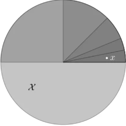
Conversely, one might ask, how many (yes/no) question are (at least) re- quired to characterize an object in given set? Assume that Alice chooses an elementx∈ X. Bob now wants to determine which element Alice has chosen.
A bad strategy would be to ask for all elementsx∈ X: have you chosen x?
Until Alice eventually says yes. Instead, one could divide the setX into sub- sets of equal size and ask in which one the chosen element was, as shown in Figure 2.1. The number of questions to be asked is then again
Number of questions =log2|X |
These considerations motivate Hartley’s formula for the uncertainty or en- tropy of a uniform random variableX overX, with PX(x) = 1/|X |, is
H(X) = log2|X |
in units of bits. Suddenly, uncertainty is a function of a random variable. The connection to probability theory is explained below. For now, consider the special case of a uniform random variable over the setX just as another way of stating that Bob has no information about Alice’s choice.
Why the logarithm? Apart from arguing with (yes/no) games, why should we use the logarithm for a measure of uncertainty? First, the uncertainty is supposed to be monotone with the size of the sample space |X |. Second, the entity is supposed to be additive for joint distributions. For two sample spaces
x
X
Figure 2.1: Strategy for determining an element that was previ- ously chosen uniformly at random.
X andYand a uniform random variableZ withP(x∧y) = 1/(X ·Y), Hartley’s formula yields
H(Z) = log2(|X | · |Y|) = log2|X |+ log2|Y|=H(X) +H(Y)
2.2.3 Connection to Probability Theory
Bob’s prior knowledge about Alice’s choice can formally be described by a probability distribution. If Bob does not know anything about Alice’s choice, each element inX was equally likely to be chosen by Alice. Thus Bob’s knowl- edge corresponds to a uniform random variable over X. The other extremal case is that Bob already knows which element Alice has chosen. This would then correspond to a deterministic probability distribution with PX(x) = 1 for one particular x ∈ X and PX(x) = 0 for all others. If Bob had known that Alice had chosen a word from an English dictionary, assuming that X contained all sequences up to 30 letters, then the probability distribution was uniform on the subset containing all dictionary words with less then 30 char- acters and zero for all other letter sequences. Bob might further be aware that Alice chooses her element according to the distribution of words in the English language. Frequent words like “the” or “and” are more likely to occur than for instance “supercalifragilisticexpialidocious.”
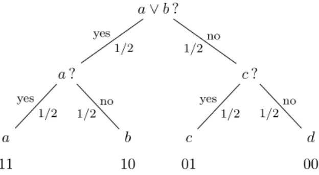
Formal characterization of the entropy For a general (not necessarily uniform) random variable X, the measure of uncertainty, i.e., the entropy, should correspond to the expectation value of the number of (yes/no) ques- tions to find an element x ∈ X using an optimal strategy and combining asymptotically many realisations of X.
a∨b?
a?
a 11
yes 1/2
b 10
no 1/2
yes 1/2
c?
c 01
yes 1/2
d 00
no 1/2 no
1/2
Figure 2.2: Strategy of determining a randomly chosen element in X. Below the final result the binary representation of the sequence of answers is given. This could be regarded as the code representation of the particular element.
Example 2.2.1 (Entropy for uniform random variable). Let us consider a ran- dom variableX overX ={a, b, c, d} withPX(x) = 1/4. A strategy similar to the one mentioned above yields the entropyH(X) = 2. It can be shown that the strategy we have employed here is optimal.
Example 2.2.2 (Entropy for non-uniform random variable). If we change the distribution of the random variable, the strategy used above is not optimal anymore. So, let us modify the probabilities to
PX(a) = 1
2, PX(b) = 1
4, PX(c) =PX(d) =1 8
Now, it is better to ask whetherais the right solution right away, as in half of the cases this will actually be right.
The expectation value of the number of question is slightly more compli- cated compared to the previous case
E[# questions] = 1 2 ·1 + 1
4·2 +1 8 ·3 + 1
8·3
= 1
2 1
·1 + 1
2 2
·2 + 1
2 3
·3 + 1
2 3
·3
=
x∈X
PX(x) log2 1
PX(x)
= 7 4 <2.
Again, the strategy turns out to be optimal, though the proof is not given here.
The entropy is smaller than in the uniform case. This fits the intuition that the uniform distribution corresponds to the least knowledge or the largest
a?
a 1
yes
b?
b 01
yes
c?
c 001
yes
d 000
no no no
Figure 2.3: Questioning strategy for a non-uniform probability distribution. Again the binary codes are given below.
uncertainty. Deviating from the uniform distribution gives more and more information. The extreme case is finally the deterministic one, with one value occurring with probability 1, whereas all the others never happen at all. Then we do not even need one single question and the entropy is zero.
In both examples, the number of questions to determine a particular ele- ment corresponds to the length of the codeword representing the element in binary digits, i.e., bits. As in the last example, the optimal length of the codeword is given by
lc(x) = log2 1
PX(x)
=−log2(PX(x)). Thus, we can now formally define the entropy.
Definition 1 (Entropy). The entropy of a random variableX overX with a distributionPX(x) =px, is given by
H(X) =E[−log2PX(x)] =−
x∈X
pxlog2px.
In case of a uniform distribution, the entropy of a random variable is the size of its range. This can be carried over to thermodynamics: “The entropy of a macrostate is the logarithm of the number of microstates corresponding to it.” The microstate of a physical system,e.g., a gas, specifies the position and momentum of each of the molecules. A macrostate, on the other hand, is simply a set of microstates, typically with a short description, such as:
“Helium gas at temperature 300 K in a cubic container of volume 100 liters and pressure 2 bar.” So if all microstates in a macrostate “look roughly the same” — this latter condition is the translation of the uniformity condition for Hartley’s formula above — we have2
H(macrostate)≈log2(# of corresponding microstates).
The “physical entropy,” as opposed to the information-theoretic one, is usually calledSand has an additional factor ofkln 2, wherekis Boltzmann’s constant (≈1.38·10−23Joule/Kelvin) and ln(2) is a common view at the border between nature and abstraction since 2 is a logical but not a natural constant.
Let us look at some examples. In the first one, we consider a “one-molecule gas” in a container of volume V, where the first macrostate corresponds to the particle being anywhere in the container, where for the other, smaller macrostate, the single particle is in the left half of the container.
Two remarks: Obviously, not all microstates in a macrostate look the same;
for instance, it is probably likelier that the particle is close to the middle of the container than to one of its corners. Second, we cannot simplycount the number of possible positions since it is infinite for both macrostates. Indeed, there also exist definitions of entropy for the continuous case, but we do not need that here as long as we are solely interested in entropydifferences: Let us assume that we distinguish different microstates only up to some fixed finite precision,i.e., we put a grid of a certain “density” into the respective volumes, and the particle’s position is described by such a grid point.
Then — whatever that density —there are exactlytwice as many microstates corresponding to the first marcostate as to the second; the entropy difference isone (bit)∆H=−1, or, renormalized, ∆S =−kln 2.
2There is something strange about this definition, namely, the apparent arbitrariness of how to assemble microstates together into macrostates. For instance — extremal example — if each macrostate corresponds to exactly one microstate, the entropy is always zero. Thus, the second law holds then, but it does not mean much. Maybe the macrostates correspond toall we knowabout a system. But then, the second law talks aboutour knowledgerather than the state of the system itself. Maybe we would like the macrostate to have a short description, as in the example above. This may work for equilibria — but is the second law not much more general?
Let us look again at the gas withN molecules.
probable improbable
work can be extracted prob. 2−N
The entropy difference here is
∆S=−N kln 2.
We can say that the transition that isprobable can also be said to allow for gaining work. Accordingly, we can of course enforce the “improbable”
transition, for instance, by pushing a piston. The gas then ceases to be a closed system, so there is no contradiction. The price we have to pay for the compression is a certain amount of free energy. The contradiction to the second law is then avoided by that amount of energy being dissipated as heat to the environment, increasing the entropy around the gas container.
∆S <0 work ∆Q
heat ∆Q tempT
∆S≤0
In the gas, the entropy decreases. A certain amount of work ∆Qis invested to force that decrease, which is then dissipated as heat to the environment.
It is that heat dissipation that, after thermalization, is responsible for the compensation — in the form of an entropy increase in the environment — of the entropy decrease in the gas. Quantitatively, the entropy increase in a heat reservoir of temperature T, which receives an amount of ∆Qof heat energy at most equal to a value proportional to 1/T, and Boltzmann’s constant is defined such that we have
∆S≤∆S T .
Taken together, the minimal investment in terms of free energy to enforce that entropy decreases is, hence,
∆Q≥∆S·T .
Let us switch back to the example of the one-molecule gas. If we interpret the molecule as storing one bit, 0 if it is on the left and 1 on the right, then forcing the molecule to the left corresponds to theerasure of that bit, in the