Structural Decoupling, Unique Solvability, Convergence Theory and Half-Explicit Methods
DISSERTATION
zur Erlangung des akademischen Grades Dr. rer. nat.
im Fach Mathematik eingereicht an der
der Mathematisch-Naturwissenschaftlichen Fakult¨at der Humboldt-Universit¨at zu Berlin
von
Dipl.-Math. Lennart Jansen
Pr¨asident der Humboldt-Universit¨at zu Berlin:
Prof. Dr. Jan-Hendrik Olbertz
Dekan der Mathematisch-Naturwissenschaftlichen Fakult¨at:
Prof. Dr. Elmar Kulke Gutachter/Gutachterin:
1. Prof. Dr. Caren Tischendorf 2. Prof. Dr. Volker Mehrmann 3. Prof. Dr. Claus F¨uhrer eingereicht am: 16.06.14
Tag der Verteidigung: 13.10.14
Diese Arbeit befasst sich mit Differential-algebraischen Gleichungen (DAEs). DAEs spie- len eine wichtige Rolle in der Modellierung, der Simulation und der Optimierung von Netzwerken und gekoppelten Problemen in vielen Anwendungsgebieten. In dieser Arbeit sind die gekoppelten Probleme aus der elektrischen Schaltungssimulation die zentrale An- wendung. Es werden in Bezug auf die Modellierung und die numerische Simulation von DAEs bereits bestehende Ergebnisse diskutiert und erweitert. Des Weiteren wird die glo- bale eindeutige L¨osbarkeit und die Sensitivit¨at der L¨osungen mit Hinsicht auf St¨orungen der DAEs untersucht.
H¨aufig wird die Modellierung von multiphysikalischen Anwendungen durch die Kopplung mehrerer einzelner DAE Systeme realisiert. Diese Herangehensweise kann hochdimensio- nale DAEs erzeugen, welche aufgrund von Instabilit¨aten nicht von klassischen numerischen Methoden, wie den BDF-Methoden, simuliert werden k¨onnen. Angesichts dieser Heraus- forderungen werden drei Ziele formuliert: Erstens wird ein globales L¨osungs-theorem for- muliert und bewiesen, welches auf gekoppelte Systeme angewandt werden kann, um deren Kopplungsansatz mathematisch zu rechtfertigen. Zweitens werden numerische Methoden vorgestellt, welche unter wesentlich schw¨acheren Strukturannahmen stabil sind und sich daher f¨ur die Simulation von gekoppelten Systemen eignen. Drittens wird eine Strate- gie pr¨asentiert, die es erm¨oglicht, explizite Methoden auf gekoppelte Systeme aus der Schaltungssimulation anzuwenden.
Eines der wichtigsten Werkzeuge, um diese Ziele zu erreichen sind die Indexkonzepte f¨ur DAEs. Zwei der bekanntesten Indexkonzepte sind der Tractability Index und der Stran- geness Index. Beide k¨onnen als Entkopplungsverfahren verstanden werden. Hier wird ein neues Indexkonzept vorgestellt, welches im Folgenden als der Dissection Index be- zeichnet wird. Die Definition eines neuen Indexkonzepts wirft unweigerlich die Frage auf:
Warum braucht man ein weiteres Indexkonzept? Um die oben gestellten Ziele zu errei- chen, braucht man ein Entkopplungsverfahren, welches die folgenden drei Eigenschaften erf¨ullt: Die Komplexit¨at des Entkopplungsverfahrens sollte nicht die Komplexit¨at der DAE ¨uberschreiten. Das Entkopplungsverfahren sollte Eigenschaften wie Symmetrie, Mo- notonie und positive Definitheit erhalten. Das Entkopplungsverfahren sollte durch einen Schritt-f¨ur-Schritt Ansatz mit unabh¨angigen Schritten realisiert werden. Sowohl das Kon- zept des Tractability Index als auch das des Strangeness Index liefert kein solches Ent- kopplungsverfahren. Der Dissection Index hingegen kann ein solches erzeugen, wie in dieser Arbeit zu sehen sein wird. Alle theoretischen Ergebnisse dieser Arbeit werden auf gekoppelte Probleme aus der Schaltungssimulation angewandt.
This thesis addresses differential-algebraic equations (DAEs). They play an important role in the modeling, simulation and optimization of networks and coupled problems in various applications. The main application in this thesis are coupled problems in electric circuit simulation.
We discuss and extend existing results regarding the modeling and numerical simulation of DAEs. Furthermore, we investigate the global unique solvability and the sensitivity of solutions with respect to perturbations of DAEs.
Nowadays the modeling of multi-physical applications is often realized by coupling sys- tems of DAEs together with the help of additional coupling terms. This approach may yield high dimensional DAEs which cannot be simulated, due to instabilities, by standard numerical methods. Regarding these challenges we formulate three objectives: First we provide a global solvability theorem which can be applied to coupled systems to mathe- matically justify their coupling approach. Second we introduce numerical methods which are stable without needing any structural assumptions. Third we provide a way to apply explicit methods to coupled systems to be able to handle the size of the coupled systems by parallelizing the algorithms.
One of the most important tools to achieve these objectives are the index concepts for differential-algebraic equations. Two of the most popular index concepts are the Tractabil- ity Index and the Strangeness Index. They both provide a decoupling procedure. Here we introduce a new index concept which we will call the Dissection Index. The definition of a new index concept inevitably invokes the following question: Why do we need another index concept?
To achieve the objectives stated above, we need a decoupling procedure which fulfills the following three properties: The complexity of the decoupling procedure has to reflect the complexity of the DAE, i.e. the decoupling procedure should be state-independent if pos- sible. The decoupling procedure should preserve properties like symmetry, monotonicity and positive definiteness. The decoupling procedure should be realized by a step-by-step approach with independent stages.
Both the Tractability Index concept and the Strangeness Index concept do not provide such a decoupling procedure. Whereas the Dissection Index does, as we will see in this thesis.
The theoretical results in this thesis will be applied to coupled problems in the electric circuit simulation.
There are many people who truly deserve to be mentioned in this acknowledgement. But in comparison to the support my mother has given me throughout my entire life, the support of these beloved and helpful people seems to fade.
And therefore everything left to say is:
Thank you, mother. You are awesome.
Lennart Jansen
Berlin, June 16th, 2014.
1 Introduction 1 2 An Introduction to Differential-Algebraic Equations 5
2.1 Explicit ODEs vs. DAEs . . . 5
2.2 Differentiation Index . . . 20
2.3 Strangeness Index . . . 22
2.4 Tractability Index . . . 25
2.5 Summary and Outlook . . . 31
3 Fields of Application 33 3.1 Circuit Applications . . . 33
3.1.1 Basic Elements . . . 35
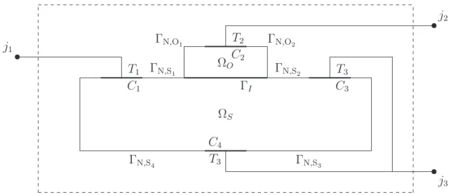
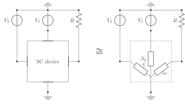
3.1.2 Semiconductor Device Model . . . 37
3.1.3 Memristor Model . . . 54
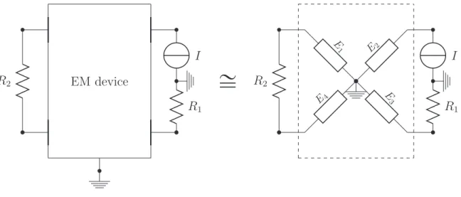
3.1.4 Electromagnetic Device Model . . . 55
3.1.5 Modified Nodal Analysis . . . 59
3.2 Mechanical Applications . . . 62
3.3 Summary and Outlook . . . 63
4 The Concept of the Dissection Index 65 4.1 Dissection Index . . . 72
4.2 Relations between Index Concepts . . . 100
4.3 Dissection Index for Circuit Applications . . . 107
4.4 Perturbation Analysis: Nonlinear DAEs . . . 115
4.5 Dissection Index for DAEs in Hessenberg Form . . . 132
4.6 Perturbation Analysis: Hessenberg DAEs . . . 138
4.7 Summary and Outlook . . . 141
5 Solvability and Uniqueness 143 5.1 Algebraic equations . . . 145
5.2 Implicit ODEs . . . 148
5.3 General DAEs . . . 150
5.4 Circuit Equations . . . 161
5.5 Summary and Outlook . . . 167
Contents
6 Convergence Analysis 169
6.1 Implicit Methods . . . 182
6.2 Left-discontinuous Collocation Methods . . . 189
6.3 Summary and Outlook . . . 208
7 Half-explicit Methods 211 7.1 Topological Decoupling . . . 211
7.1.1 Topological basis functions . . . 212
7.1.2 Extended MNA with controlled sources . . . 213
7.1.3 Extended MNA without controlled sources . . . 216
7.2 Explicit Methods . . . 220
7.3 Summery and Outlook . . . 234
8 Conclusion and Outlook 235
This thesis addresses differential-algebraic equations (DAEs). They play an important role in the modeling, simulation and optimization of networks and coupled problems in various applications, e.g. integrated circuit design, hydraulic engineering, mechanical en- gineering and medicine. Often, the model equations lead to a partial differential-algebraic equation system (PDAE) meaning a mix of ordinary differential equations, partial dif- ferential equations and algebraic constraints. We focus our investigations on general differential-algebraic equations resulting from a spatial discretization of such PDAEs. We discuss and extend existing results regarding the modeling and numerical simulation of DAEs. Furthermore, we investigate the global unique solvability and the sensitivity of solutions with respect to perturbations of DAEs.
Nowadays the modeling of multi-physical applications is often realized by coupling systems of DAEs together with the help of additional coupling terms. This approach may yield high dimensional DAEs which cannot be simulated, due to instabilities, by standard numerical methods. In particular we will
1. provide a global solvability theorem which can be applied to coupled systems to mathematically justify their coupling approach.
2. provide numerical methods which are stable under almost no structural assumptions.
3. provide a way to apply explicit methods to coupled systems to be able to handle the size of the coupled systems by parallelizing the algorithms.
One of the most important tools to achieve these objectives are the index concepts for differential-algebraic equations. There are already many different index concepts avail- able. The Differentiation Index is probably the best known index, since its concept is rel- atively demonstrative. It was introduced by Petzold and Campbell, see [Cam87, BCP96].
The Perturbation Index measures the degree of the influence of the derivatives of per- turbation to the solution of a DAE. It was initially defined in [HLR89]. Two of the most popular index concepts are the Tractability Index [GM86, M¨ar02, LMT13] and the Strangeness Index [KM06]. They both provide a decoupling procedure. All of these index concepts have their own advantages and disadvantages. Here we introduce a new index concept which we will call the Dissection Index. The definition of a new index concept inevitably invokes the following question: Why do we need another index concept?
To achieve the objectives stated above, we need a decoupling procedure which fulfills the following properties:
1. The complexity of the decoupling procedure has to reflect the complexity of the DAE, i.e. the decoupling procedure should be state-independent if possible.
2. The decoupling procedure should preserve properties like symmetry, monotonicity and positive definiteness.
3. The decoupling procedure should be realized by a step-by-step analysis with inde- pendent stages.
Both the Tractability Index concept and the Strangeness Index concept do not provide such a decoupling procedure. Whereas the Dissection Index does, as we will see in this thesis.
The Dissection Index can be interpreted as a mix of the Tractability Index and the Strangeness Index. The index arises as we use the linearization concept of the Tractability Index and the decoupling procedure of the Strangeness Index. The Strangeness Index uses basis functions for its decoupling procedure while the Tractability Index uses projectors for this purpose. The advantage of projector functions is that they need less assumptions regarding the domain to be differentiable. Nevertheless, we favor basis functions since they preserve the original size of the equations while splitting them.
This thesis is structured as follows. After presenting well-known results and facts of differential-algebraic equations, we introduce the concepts of the Strangeness Index and the Tractability Index. Before we define our new index concept, we present and model the application classes which will be discussed in this thesis. These classes are electrical circuits including semiconductor devices, memristors and electromagnetic devices and mechanical multibody systems.
After introducing our new index concept and proving that it is well defined, we will analyze the sensitivity to perturbations of differential-algebraic equations. In contrast to ordinary differential equations, which can be interpreted as integral problems, differential-algebraic equations may contain differentiation problems. The appearance of these differentiation problems leads to an ill-posed problem, in the sense of Hadamard, if we consider per- turbed input data, see [LRS86]. Even very small perturbations can have arbitrarily large derivatives and therefore small perturbations may have a huge influence on the solution of a differential-algebraic equation. Hence it is necessary to analyze the sensitivity to perturbations of DAEs.
In case of the perturbation analysis and also for the convergence theory it is necessary to assume that the unperturbed DAE has a global unique solution. Furthermore, we need to prove the global unique solvability of our considered coupled systems to mathematically
justify their coupling approach. We will provide sufficient criteria for the global unique solvability of differential-algebraic equations with an arbitrary index. To do so we need insight of the structure of the differential-algebraic equation to apply the established solvability theories of ordinary differential equations and algebraic equations. To obtain this needed insight we make use of the Dissection Index concept.
The remaining two chapters deal with challenges of the applicability, the stability and the convergence of numerical methods. It is known that standard ODE methods like the implicit Euler methods, the BDF methods or the Radau IIA methods may loose their convergence if applied to DAEs, cf. [GP83, LMT13]. These standard ODE methods have a basic flaw: They do not reflect the product rule properly. This is not a problem as long as these methods are applied to ODEs. When we consider a DAE it may happen that the kernels, which describe the inner structure of a DAE, are not constant. If these kernels are also involved in a differentiation problem then hidden differentiations of products of functions might occur which leads to the instability of these standard ODE methods. We will introduce a class of methods which reflects the product rule properly and thereby overcomes these instability problems. In particular this will make the reformulation of the DAE superfluous.
In the last chapter we investigate half-explicit methods applied to DAEs. Since it is no longer possible to accelerate CPUs like it has been in the past, parallelizing algorithms becomes more and more important. Because they can be paralellized very efficiently, explicit methods are being focused on even more so nowadays. Hence explicit methods are focus even more nowadays because they can be paralellized very efficiently. Half- explicit methods for DAEs are often defined for semi-explicit DAEs and therefore they are rarely used in circuit simulation in contrast to mechanical applications. We introduce a new class of half-explicit multistep methods and prove their convergence.
The main application in this thesis will be the electric circuit simulation. Electrical circuits are of great importance for industrial research and therefore a mathematical un- derstanding is needed. There already exist many works about DAE related questions regarding circuits, in particular about index analysis [Tis99, RT11] and local uniqueness and solvability [HM04, Bau12]. Besides standard elements like inductors, resistors, capac- itors and source elements, electrical circuits can also contain more complex elements like semiconductor devices, memristors and electromagnetic devices. For instance, semicon- ductor devices and electromagnetic devices are described by a set of partial differential equations, hence they involve new questions and challenges to the analysis of electri- cal circuits. Previous research about semiconductor devices can be found in [SBST14, Gaj93, Gaj94, Tis03, ABG04, ST05, Sot06, Bod07, BST10], these devices are widely used in circuits because of their application as transistors. In [Chu11, Ria11, RT11, Bau12]
memristors are investigated while we find previous research about electromagnetic devices in [HM76, KMST93, Wei77, Bau12, BBS11, Sch11].
In this thesis we will
1. apply our perturbation analysis to the circuit applications.
2. prove the global unique solvability of the coupled circuit model.
3. provide a topological decoupling into a semi-explicit DAE for the circuit applica- tions which has low computational costs and preserves the symmetry and positive definiteness of the circuit model.
4. apply our class of half-explicit methods to circuit applications.
Differential-Algebraic Equations
This chapter presents well-known results and facts for Differential-Algebraic Equations (DAEs) and lays the foundations for the following chapters.
The first part of the chapter is a general introduction to differential-algebraic equations.
It presents challenges and problems of this field with the help of small examples. This includes classical problems like the appearance of differentiation problems or the drift-off phenomenon.
Furthermore the concepts of the Differentiation Index [Cam87, BCP96], the Strangeness Index [KM06] and the Tractability Index [GM86, M¨ar02, LMT13] are introduced and discussed. These three concepts are well established analysis tools for DAEs. Their respective advantages and disadvantages will be pointed out.
2.1 Explicit ODEs vs. DAEs
Differential-algebraic equations as well as explicit Ordinary Differential Equations(ODEs) can be understood as implicit ODEs. The following definitions follow the understanding of the relations between explicit ODEs, DAEs and implicit ODEs of [LMT13].
Definition 2.1. (Implicit ODE)
Let I ĂR and Dx,Dx1 ĂRn be open subsets. We consider the following equation
Fpx1ptq, xptq, tq “0 (2.1) with a continuous function F PCpDx1ˆDxˆI,Rnq. Furthermore let F have continuous partial derivatives BBx1Fpx1, x, tq and BBxFpx1, x, tq. We call (2.1) an implicit ODE. If
BBx1Fpx1, x, tqis non-singular for all triplespx1, x, tq PDx1ˆDxˆI, we call (2.1) a regular implicit ODE.
In particular explicit ODEs are regular implicit ODEs.
Definition 2.2. (Explicit ODE)
Let I Ă R and D Ă Rn be open subsets with t0 P I and let f P CpD ˆI,Rnq be continuous. We call
x1ptq “fpxptq, tq, xpt0q “ x0 (2.2)
an explicit ODE with an initial condition. Let I‹ :“ rt0, Ts ĂI. We call x‹ PC1pI‹,Rnq a solution of (2.2) on I‹ if the initial conditions are fulfilled, i.e. x‹pt0q “ x0, and
x1‹ptq “fpx‹ptq, tq @tP I‹.
In contrast to explicit ODEs, DAEs are implicit ODEs, which are not regular.
Definition 2.3. (DAE in standard form)
Let I Ă R and Dx,Dx1 Ă Rn be open with t0 P I. Let F P CpDx1 ˆDx ˆI,Rnq be continuous such that the partial derivatives BxB1Fpx1, x, tqand BBxFpx1, x, tqare continuous with BBx1Fpx1, x, tq being singular for all triples px1, x, tq PDx1ˆDxˆI. We call
Fpx1ptq, xptq, tq “ 0, xpt0q “x0 (2.3) a DAE in standard form with initial conditions.We callx‹ PC1pI‹,Rnqa solution of (2.3) on I‹ :“ rt0, Ts ĂI if the initial conditions are fulfilled, i.e. x‹pt0q “ x0, and
Fpx1‹ptq, x‹ptq, tq “ 0 @tP I‹. We also introduce the following subclass of DAEs.
Definition 2.4. (Semi-explicit DAE)
Let I ĂR and Dx ĂRnx and Dy ĂRny be open subsets. We consider the following set of equations
x1 “fpx, y, tq (2.4a)
0“gpx, y, tq (2.4b)
with f P CpDx ˆDy ˆI,Rnxq and g P CpDx ˆDy ˆI,Rnyq. Further, let the partial derivatives of f and g, with respect to x and y, be continuous. We call (2.4) a semi- explicit DAE.
In the case of a semi-explicit DAE only the derivatives of x appear in the equations.
Therefore we call x the dynamical variables, while we call y the algebraic variables.
Analogously we call the equations (2.4a) the dynamical equations and (2.4b) the algebraic equations of the semi-explicit DAE (2.4). Hence (2.4) is a special case of a DAE in the sense that it is an implicit ODE which is not regular.
In the following we present differences between explicit ODEs and DAEs with the help of a sequence of small examples.
Solvability for Arbitrary Initial Values
There are well-known solvability results for explicit ODEs which provide criteria for the solvability with respect to an arbitrary initial valuex0 at a time pointt0. Peano’s theorem states that there is a T ą t0 such that there is at least one solution for every initial condition of the ODE on rt0, Tsif f is continuous, cf. [Aul04]. We say the ODE is locally solvable, since the solution interval rt0, Ts can be arbitrarily small. If the function f is locally Lipschitz continuous in x, this local solution becomes unique by the Picard- Lindel¨of theorem, cf. [Aul04]. If f is even globally Lipschitz continuous in x, then for every initial condition and for every time interval rt0, Ts with T ą t0 there is a unique solution of the ODE on the whole time interval rt0, Ts, cf. [GJ09].
It is not possible to formulate such results for arbitrary initial conditions in the DAE case.
We consider the following DAE as a counter example.
Example 2.5. Let I :“ rt0, Ts Ă R be a compact time interval and let t P I. Assume f :I ÑR to be continuous.
x1 “y (2.5a)
y“fptq (2.5b)
This DAE consists of one differential equation (2.5a) and one algebraic equation (2.5b).
In contrast to the solvability of explicit ODEs for arbitrary initial conditions, see Peano’s theorem and the Picard-Lindel¨of theorem, the DAE (2.5) is only solvable for initial values satisfying ypt0q “fpt0q.
Differentiation Problem
We can write an explicit ODE (2.2) in integral notation xptq “ x0`
żt t0
fpxpsq, sqds
such that we deal with an integration problem. Hence, it is possible to notate an explicit ODE (2.2) without derivatives. This is no longer the case for DAEs, in general. If we change the algebraic equation in Example 2.5 by setting xequal to f instead ofy, we get a very similar looking DAE, which has a totally different solution structure.
Example 2.6. Let I :“ rt0, Ts Ă R be a compact time interval and let t P I. Let f :I ÑR be continuously differentiable.
x1 “y x“fptq
This time the dynamical variable xis fixed algebraically. In fact all solution components are algebraically fixed, since xptq “fptq and yptq “x1ptq “f1ptq. We cannot choose any initial value freely. Additionally, y depends on the derivative of the right hand side fptq. So we are dealing with a differentiation problem instead of an integration problem. As an obvious analytic consequence, the right hand sidefptqmust be sufficiently smooth, as already mentioned in the example.
It is possible to create a differentiation problem of second order if we add one more differentiation to the equations of Example 2.6.
Example 2.7. Let I :“ rt0, Ts Ă R be a compact time interval and let t P I. Let f :I ÑR be twice continuously differentiable.
x12 “y x11 “x2 x1 “fptq
This set of equations is solved byx1 “fptq, x2 “f1ptqandy“f2ptq. Hence, the solution of y is the second derivative of f.
The appearance of differentiation problems within DAEs motivates a classification for DAEs which counts the order of the involved differentiation problem. This kind of clas- sification is called the index of a DAE. There are several different index concepts, put simply they are all intended for counting the order of the involved differentiation prob- lem. These index concepts are the most important tools of DAE analysis. We give an introduction of some of the most popular index concepts in the Sections 2.2, 2.3 and 2.4.
Numerical Approximation of the Difference Quotient
The differentiation problems in DAEs induce smoothness assumptions regarding the right hand side f. Additionally, there are numerical problems created by the differentiation problems. If we discretize Example 2.6 by the implicit Euler method and a time step size h, we obtain
xn´xn´1 h “yn
xn“fptnq,
with xn and yn being the numerical approximations of xptnq and yptnq, respectively. It follows directly that yn is given by the difference quotient of fptq attn,
yn “ fptnq ´fptn´hq
h .
The difference quotient of a differentiable function fptq at a time point tn converges to its derivative at the same time point f1ptnq, i.e.
lim
hÑ0
fptnq ´fptn´hq
h “f1ptnq.
But this convergence may fail if the difference quotient is computed on a machine with finite precision arithmetic. Numerically calculated values are only as accurate as the rounding accuracy of the used computer system. We call the rounding error δ. The rounding error can be seen as a random number in r´10´16,10´16sif one uses the double precision floating-point format. This phenomenon is called the loss of significance.
To visualize this problem let fptq “ sinptq and let δn be the rounding error of sinptnq. Then we actually calculate
yn “ sinptnq `δn´sinptn´1q ´δn´1 h
“ sinptnq ´sinptn´1q
h ` δn´δn´1 h
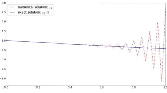
Therefore the numerical solution yn will not converge against cosptnq for h Ñ 0, since the rounding error δn´1 does not converge againstδn. In Figure 2.1 we see the numerical error en :“ |yn´cosptnq|at tn“1 for different time step sizes h.
Figure 2.1: Numerical error of the difference quotient.
This basic flaw of the difference quotient is one of the main problems in the numerical treatment of DAEs. This fact is well-known since differentiation is an ill-posed problem, in the sense of Hadamard, if it is connected with perturbed input data, see [LRS86].
Hence, small time step sizes no longer yield small errors, in general. This problem can get even worse if we consider Example 2.7. Applying the implicit Euler method again we
achieve
yn“ fptnq ´2fptn´1q `fptn´2q
h2 ,
with a constant time step size h. This confronts us with a harder version of the problem of Example 2.6, since the rounding error will be multiplied by h12.
Figure 2.2: Numerical error of the difference quotient of the second derivative.
We choose again fptq “sinptqand tn “1. Figure 2.2 describes the relation between the time step size and the accuracy of yn reflecting the second derivative of f. As soon as the step sizeh drops below 10´8 it may happen that fptnq ´2fptn´1q `fptn´2qbecomes smaller than 10´16 which then will be presented by a subnormal number. This explains the behavior of the error for time step sizes smaller than 10´8. Summarizing, this means that a high order of the differentiation problem may lead to difficulties during the solving of the DAE.
Mixed Variables
In all the previous examples it is obvious which of the variables have to be differentiable and which are directly algebraically fixed. This does not have to be the case in general and also not in most applications. We consider the following example.
Example 2.8. Let be I :“ r´1,1s and tP I.
pz0´z1q1 “z0`z1 (2.6a)
z0`z1 “4|t|. (2.6b)
The general solution of this problem is given byz0ptq “ p2`tq|t|`candz1ptq “ p2´tq|t|´c for somecP R. The initial value of eitherz0 orz1 can be chosen, but not both at the same time. So which of the solution components is algebraically fixed? They are both not fixed but the combination pz0`z1qptqis fixed, as we can see in the second equation (2.6b). This example shows also an important smoothness property of DAEs. In the examples 2.6 and 2.7 it was shown that the right hand side can underlie smoothness requirements. Now we see that smoothness properties of the variables are not trivial either. In Example 2.8 non of the solution components for themselves are even differentiable once. But there appears a derivative of a combination of the variables in the equations and this combination pz0 ´z1qptq “ 2t|t| `2c is in fact continuously differentiable. Motivated by the class of semi-explicit DAEs (2.4) we call the parts of the variables, whose derivatives appear in the equations, dynamic. The remaining parts of the variables are called algebraic. Notice that these parts must not necessarily be a set of notated variables, but they can also be combinations of the variables.
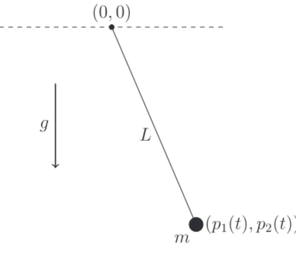
As an application example for mixed variables consider the mathematical pendulum, cf.
[Ste06]. This is one of the most basic DAE examples in mechanical applications.
Example 2.9. Let I :“ r0,2¨10´6s be the time interval.
p11 “v1 p12 “v2 mv11 “ ´2p1λ mv21 “ ´2p2λ´mg
0“p21`p22´L2
with m ą 0 being the mass of the object, g being the gravity of earth and L being the length of the pendulum.
pp1ptq, p2ptqq p0,0q
m g L
Figure 2.3: Mechanical example: mathematical pendulum
This DAE is interesting, in a mathematical point of view, because of its last equation.
Obviously it is the only algebraic equation, since m ą 0. Now the question is: Which parts of p1 and p2 are algebraically fixed? In fact the fixed combination of p1 and p2 depends on the current states of p1 and p2 themselves. Analyzing DAEs theoretically becomes much harder, if such state depending combinations show up.
Consistent Initial Values
The next two examples show what may happen during a simulation if the initial values are chosen randomly.
Example 2.10. Let I :“ r0,1s and lett PI. x12 “y x11 “ey ´1 x1 “ ´1
The exact solution of this example is given by x1ptq “ ´1, x2ptq “x02 P R, yptq “0. We assume that we do not know the exact solution but we have to choose initial values. We observe what happens if we choose x01 “0, x02 “0,y0 “0 and discretize the example by the implicit Euler scheme. First we get the discretized system for the first time step
x2,1´x2,0 h “y1 x1,1´x1,0
h “ey1 ´1 x1,1 “ ´1.
We obtain, after reorganizing the equations,
x2,1 “hy1 (2.7a)
y1 “lnp1´ 1
hq (2.7b)
x1,1 “ ´1 (2.7c)
if we then insert the chosen initial values. Since the time step size h is larger than zero it has to be larger than one because equation (2.7b) is not solvable for 0 ăhď1. But if we have to choose hą1 we cannot solve the example since the solution interval is given by I :“ r0,1s.
When at least one solution passes through an initial value, we call the initial value consis- tent, cf. [LMT13]. The initial values in Example 2.10 are inconsistent, since no solution passes through a point with x1 being zero. As in Example 2.8, the selection of the initial
values becomes a non trivial topic in practice. Dealing with an explicit ODE we can just choose initial values for all solution components, but when we deal with DAEs this is no longer the case. It can be very difficult to find any initial value due to the size of the DAEs which appear in practice.
Not only the size of a system can be a problem when we want to calculate consistent initial values. It can also be unclear which are the conditions we have to fulfill to obtain consistent initial values. In Example 2.5 the only condition is the algebraic equation (2.5b). If we choose initial values which fulfill this algebraic equation, we already get consistent initial values for this example. Conditions arising from algebraic equations are called obvious constraints. In Example 2.6 it is not enough to fulfill the obvious constraints. Here the first equation imposes an additional condition on the initial values, because of the differentiation problem. Conditions arising from dynamical equations are called hidden constraints.
In the previous example the implicit Euler failed to calculate any numerical solution of the DAE due to the choice of the initial values. In the next example inconsistent initial values are chosen again but this time the implicit Euler provides a numerical solution.
Example 2.11. Let I :“ r0,1s and lett PI. x12 “y x11 “y x1 “1
The exact solution of this example is given by x1ptq “ 1, x2ptq “ x02 P R, yptq “ 0. We observe again what happens if we choose x01 “ 0, x02 “c P R, y0 “0 and discretize the example with the implicit Euler scheme. With the first Euler step we obtain
x2,1 “c`hy1 y1 “ 1
h x1,1 “1.
While for a general n ě1 we get
x2,n´x2,n´1 h “yn x1,n´x1,n´1
h “yn x1,n “1 which leads to
x2,n “x2,n´1 “c`1
yn“0 x1,n “1
for n ě2. In this case the Euler indeed calculates a numerical solution but this solution does not converge against the exact solution in the x2 component regarding the initial value. The inconsistent choice of the initial values altered the trajectory of the x2 com- ponent independently of h. Therefore Example 2.11 is even more vicious than Example 2.10 because this time the problem is not obvious.
Explicit Methods
Another challenge in the field of DAE numerics is the usage of explicit methods, cf.
[ASW93, BH93, Arn98, Mur97, Ost93]. Even in Example 2.5 an explicit method cannot be used without extra efforts. Using the explicit Euler scheme we obtain
xn´xn´1
h “yn´1 yn´1 “fptn´1q.
Since yn does not appear in these equations, obviously it is not possible to solve these equations with respect to xn and yn. Of course, in this case we could just discretize the differential equation explicitly while we treat the algebraic one implicitly, i.e. we evaluate it in tn, and obtain
xn´xn´1
h “yn´1 yn“fptnq.
But this approach does not work for Example 2.6. Even if we evaluate the algebraic equation in tn, the variable yn still does not appear in the equations.
xn´xn´1
h “yn´1 xn“fptnq.
Variable Time Step Size
Not only explicit methods are more difficult to use, also non constant time step size becomes harder to apply, cf. [LMT13]. If we consider Example 2.7 we are dealing with a second order differentiation problem. The problem is that even analytically the difference quotient for the second derivative converges only for a constant time step size regardless of the rounding error. So if there is at least a second order differentiation problem involved
in a DAE the usage of numerical solvers with a variable time step size is not trivial. We apply the implicit Euler method on the equation of Example 2.7
x12 “y x11 “x2 x1 “fptq and obtain the time discretized version
x2,n´x2,n´1 hn “yn x1,n´x1,n´1
hn “x2,n x1,n “fptnq.
After reorganization we achieve an explicit description for the numerical solution x1,n “fptnq
x2,n “ fptnq ´fptn´1q hn yn“
fptnq´fptn´1q
hn ´fptn´1hq´n´1fptn´2q
hn .
We define h“maxphn´1, hnq, then there is acą0 such that we can write yn “ hn`hn´1
2hn f2ptnq `Ophq with the help of a Taylor series as long as hhn
n´1 ď c and hhn´1
n ďc. That directly tells us that the difference
yptnq ´yn“ hn´hn´1
2hn f2ptnq `Ophq
will converge against zero for any function f PC2pR,Rq if and only ifhn“hn´1.
Convergence Problems for Classical ODE Methods
Next we consider an example from [GP83] in standard formulation.
Example 2.12. Let I :“ r0,3s and lett PI.
x11 `ηtx12 “ ´p1`ηqx2 x1 `ηtx2 “e´t
The main difference to the previous example is the time dependency of the coefficients.
This example is of huge numerical significance because the implicit Euler fails to solve it if we chooseη ă ´12. This holds even if we use a constant step size and choose consistent initial values.
Figure 2.4: Numerical and exact solutions of theη-DAE withη“ ´0.55 using the implicit Euler.
Hence we can no longer rely on classical methods like the implicit Euler in general. An other alarming behavior of the η-DAE is, that for η ě ´12 the example is very easy to solve with the implicit Euler. This shows that the numerical complexity may depend on parameters like η.
Asymptotic Instability
The next example is an electric circuit, which is called the Miller Integrator, cf. [MG05, Pul12]. The corresponding equations are given by:
Example 2.13. Let I :“ r0,2¨10´6s and lett PI.
Gpe1´e2q `jv1 “0 pC1`C2qe12 ´C2e13´Gpe1 ´e2q “ 0 C2pe3´e2q1`jv2 “0
e1 “uinptq e3´2e2 “0,
where theei are the electrical potentials at the nodes and the jvi are the currents over the voltage source and the operational amplifier. Further uinptqis the voltage of the voltage source which we set to uinptq “sinp2π106tq.
uinptq jv1
G
C1
C2
´
`
jv2
e1 e2 e3
We transform and factorize the equations of Example 2.13 to determine the order of the differentiation problem in the example.
jv1 “Gpe2´uinptqq (2.8a)
e1 “uinptq (2.8b)
e3´2e2 “0 (2.8c)
´C1
Gpe3´2e2q1` C2´C1
GC2 jv2`e2 “uinptq (2.8d) C2pe3´2e2q1`C2e12`jv2 “0, (2.8e) Equation (2.8d) yields a description of jv2 depending on the first derivative of e3´2e2
jv2 “ GC2
C2´C1puinptq ´e2`C1
Gpe3´2e2q1q if C2 ‰C1. But for C2 “C1 we obtain
e2 “uinptq ` C1
Gpe3´2e2q1 C2pe3´2e2q1`C2e12`jv2 “0,
which yields
jv2 “ ´C2pe3´2e2q1´C2pu1inptq ` C1
Gpe3´2e2q2q.
Therefore this problem contains a second order differentiation problem for C2 “ C1. But for every other case, i.e. C2 ‰ C1, it contains a first order differentiation problem.
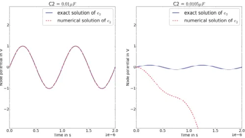
We choose G“ 1kΩ1 and C1 “0.01μF, then only for C2 “ 0.01μF there is an order two differentiation problem within these equations. If we changeC2 slightly toC2 “0.0105μF, there is an order one differentiation problem in the equations. We see that the lower order differentiation problem gives us much more trouble if we solve this circuit for the two different sets of parameters, see Figure 2.5.
While the second order differentiation problem gives us a stable solution, even for rela- tively large time step sizes, the first order differentiation problem always drifts off regard- less of how small we choose the time step size.
Figure 2.5: Numerical stability issues of the the Miller Integrator
To understand this behavior we examine the equations, which describe the potential e2 for the different parameter sets. For C2 “C1 it holds
e2 “uinptq
while we obtain
e12 “ G
C2´C1e2 ´ G
C2´C1uinptq (2.9)
for C2 ‰C1. The solutions of the homogeneous version of (2.9) are e2,hptq “ ceC2G´C1t
with c depending on the initial condition. For C2 slightly larger than C1 the function e2,hptq grows extremely fast. This instability in the homogeneous solutions is the reason for the drift off in Example 2.13.
The same problem can occur if we switch an algebraic equation with its derivative. We consider the following equation
eλtx“epλ´1qt (2.10)
Its solution is given by
xptq “e´t
and if we solve this numerically withλ“ ´15 inI “ r0,2swe obtain a numerical solution which is similar to the exact solution.
If we want to express the same problem with a dynamical equation instead of an algebraic one, we differentiate (2.10) and obtain:
λeλtx`eλtx1 “ pλ´1qepλ´1qt (2.11)
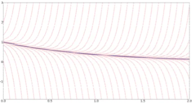
or even more simple x1 “ ´λx` pλ´1qe´t. This ODE is solved by xptq “ e´t`ce´λt depending on the initial value x0 at t0 “0.
Figure 2.6: Solution trajectories of the dynamical equation
If we choose x0 “1, then the ODE (2.11) is solved by x‹ptq “e´t just like the algebraic equation. For λ“ ´15 andI “ r0,2s we obtain an unstable solution again.
Figure 2.7: Stability behavior of the algebraic and the dynamical equation.
The reasons for this drift off phenomenon are again the unstable solution trajectories of the ODE (2.11). If we solve (2.11) by the implicit Euler or any other numerical method, we make a small error in every time step. In this particular case this small error is the reason why the numerical solution leaves the stable solution trajectory. Once on this unstable solution trajectory, the numerical solution grows unbounded.
As already mentioned, the differentiation problems involved in the DAEs motivate a clas- sification. In the following we introduce three of the most popular classification concepts:
The Differentiation Index, the Strangeness Index and the Tractability Index.
2.2 Differentiation Index
In this section we introduce the Differentiation Index for nonlinear DAEs in standard form.
The Differentiation Index is probably the best known index, since its concept is relatively demonstrative. It was introduced by Petzold and Campbell, see [Cam87, BCP96]. To define the Differentiation Index we need the DAE (2.3) itself but also its derivatives. For a compact notation we define the inflated system.
Definition 2.14. (Inflated system - [KM06], p.153)
Considering the DAE (2.3) we gather the original equation and its derivatives up to order ν PN0 into an inflated system
Fνpxpν`1qptq, ..., x1ptq, xptq, tq “0, (2.12) where Fν has the form
Fνpxν`1, ..., x1, x, tq “
»
—–
Fpx1, x, tq
BBx1Fpx1, x, tqx2` BBxFpx1, x, tqx1`BBtFpx1, x, tq ...
fi ffifl
and define the Jacobians
Gpx1, x, tq “ B
Bx1Fpx1, x, tq Bpx1, x, tq “ B
BxFpx1, x, tq Gνpxν`1, ..., x1, x, tq “ B
Bpx1, . . . , xν`1qFνpxpν`1q, ..., x1, x, tq Bνpxν`1, ..., x1, x, tq “ B
BxFνpxν`1, ..., x1, x, tq.
Over the years the definition of the Differentiation Index has been slightly modified to adjust from the linear to the nonlinear case [Cam87, CG95b, CG95a] and to deal with slightly different smoothness assumptions. We concentrate only on the nonlinear case and define the Differentiation Index with the help of the inflated system.
Definition 2.15. (Differentiation Index)
The DAE (2.3) has Differentiation Index μ, if and only if F P CμpDx1ˆDxˆI,Rnqand μ is the minimal number such that an explicit ODE x1 “ fpx, tq can be extracted from Fμpxpμ`1q, ..., x1, x, tq “0 by algebraic manipulations only with f being continuous.
In a way the Differentiation Index measures the difference of a DAE to an explicit ODE by counting the number of differentiations needed for the transformation to an explicit ODE. Previously we talked about differentiation problems within a DAE. One could also say that the Differentiation Index tries to count the order of these differentiation problems. Lets take a look at a small example to get to know the inflated system and the Differentiation Index.
Example 2.16.
For tP r0,10sconsider the DAE
px0`x1q1 “x1 x0 `x1 “sinptq.
If we differentiate the system two times we get the inflated system px0`x1q1 “x1
x0`x1 “sinptq px0`x1q2 “x11
px0`x1q1 “cosptq px0`x1q3 “x21
px0`x1q2 “ ´sinptq.
With these equations we achieve by algebraic manipulations x10 “x1 `sinptq
x11 “ ´sinptq.
and therefore the DAE has at most Differentiation Index index 2. To guarantee that the index is not smaller than 2, we would have to check that it is not possible to create an explicit ODE with just one or none differentiation.
The major advantage of the Differentiation Index is its simple and demonstrative concept.
In return the Differentiation Index concept has two major drawbacks.
First it is hard to determine whether or not the used number of differentiations is the minimal one to obtain an explicit ODE. Although it may be easy to calculate an upper bound of the Differentiation Index, to assure that the used number of differentiations is the minimal one we would have to check all smaller cases. This may become difficult and time-consuming.
And secondly the Differentiation Index needs more smoothness than necessary as we see in the next example.
Example 2.17.
For tP r´1,1s consider the DAE
x10´x1 “0
x0`x2 “sinptq ` |t| x2 “ |t|.
The Differentiation Index is at least one, since the derivatives ofx1 andx2 do not appear in the equations. So we need to differentiate the equations at least once, which is not possible since |t| is only continuous.
2.3 Strangeness Index
In this section we introduce the concept of the Strangeness Index for nonlinear DAEs in standard formulation. The Strangeness Index was first established by Kunkel and Mehrmann, see [KM06]. The Strangeness Index can be considered as a generalization of the Differentiation Index. It also uses the inflated system to analyze the structure of a DAE. The following definition of the Strangeness Index seems to be more technical than the definition of the Differentiation Index, but if we look closely they are strongly related.