Assessing Policy Quality in Multi-stage Stochastic Programming
Anukal Chiralaksanakul and David P. Morton Graduate Program in Operations Research
The University of Texas at Austin Austin, TX 78712
January 2003
Abstract
Solving a multi-stage stochastic program with a large number of scenarios and a moderate-to- large number of stages can be computationally challenging. We develop two Monte Carlo-based methods that exploit special structures to generate feasible policies. To establish the quality of a given policy, we employ a Monte Carlo-based lower bound (for minimization problems) and use it to construct a confidence interval on the policy’s optimality gap. The confidence interval can be formed in a number of ways depending on how the expected solution value of the policy is estimated and combined with the lower-bound estimator. Computational results suggest that a confidence interval formed by a tree-based gap estimator may be an effective method for assessing policy quality. Variance reduction is achieved by using common random numbers in the gap estimator.
1 Introduction
Multi-stage stochastic programming with recourse is a natural and powerful extension of multi-period deterministic mathematical programming. This class of stochastic programs can be effectively used for modeling and analyzing systems in which decisions are made sequentially and uncertain parameters are modeled via a stochastic process. The timing of making a decision and observing a realization of the uncertain parameters is a key feature of these models. At each stage, a decision, subject to certain constraints, must be made with information available up to that stage, while the future evolution of the stochastic process is known only through a conditional probability distribution. The goal is to find a solution that optimizes the expected value of a specified performance measure over a finite
which specifies what decision to take at each stage, given the history of the stochastic process up to that stage.
Multi-stage stochastic programming with recourse originated with Dantzig [10], and has been applied in a variety of fields ranging from managing financial systems, including asset allocation and asset-liability management, to operating hydro-thermal systems in the electric power industry to sizing and managing production systems. See, for example, Birge and Louveaux [3], Dupaˇcov´a et al. [19], Dupaˇcov´a [20], Kall and Wallace [36], Pr´ekopa [48], Wallace and Ziemba [56], and Ziemba and Mulvey [59].
When the underlying random parameters have a continuous distribution, or finite support with many realizations, it is usually impossible to evaluate the expected performance measure exactly, even for a fixed solution. This is true for one- and two-stage stochastic programs. Computational difficulties are further compounded in the multi-stage setting, in which the stochastic program is defined on a scenario tree, and problem size grows exponentially with the number of stages. As a result, there is considerable interest in developing approximation methods for such stochastic programs.
Approximation methods for multi-stage stochastic programs often utilize exact decomposition algorithms that are designed to handle multi-stage problems with a moderate number of scenarios.
We call an optimization algorithm “exact” if it can solve a problem within a numerical tolerance.
Exact decomposition algorithms can be broadly divided into two types: those that decompose by stage and those that decompose by scenario. The L-shaped method for multi-stage stochastic linear programs [2, 25] is a by-stage decomposition scheme. One of the approximation methods we develop in this paper is based on a multi-stage L-shaped method. By-scenario decomposition algorithms include Lagrangian-based methods [44, 49].
When a multi-stage stochastic program is too large, due to the number of scenarios, to be solved exactly one may approximate the scenario tree to achieve a problem of manageable size. Schemes to do so based on probability metrics and moment matching are described in [9, 18, 32, 47]. Bound- based approximations of scenario trees exploit convexity with respect to the random parameters; see [5, 21, 22, 23].
Another type of approximation is based on Monte Carlo sampling, and these methods can be further categorized by whether the sampling is performed “inside” or “outside” the solution algorithm.
Internal sampling-based methods replace computationally difficult exact evaluations with Monte Carlo estimates during the execution of the algorithm. For multi-stage stochastic linear programs, several variants of internal sampling-based L-shaped methods have been proposed. Pereira and Pinto [46]
estimate the expected performance measure by sampling in the forward pass of the L-shaped method.
Their algorithm can be applied to stochastic linear programs with interstage independence that have many stages but a manageable number of descendant scenarios at each node in the scenario tree.
Linear minorizing functions, or cuts, on the expected performance measure are computed exactly in the backward pass, and can be shared among subproblems in the same stage due to interstage
independence. Donohue’s [16] “abridged” version of this algorithm reduces the computational effort associated with each iteration. Chen and Powell [6] and Hindsberger and Philpott [31] have developed related algorithms. Convergence properties for this class of algorithms are addressed in Linowsky and Philpott [41]. Dantzig and Infanger [12, 34] employ importance sampling in both forward and backward passes of a multi-stage L-shaped method for stochastic linear programs with interstage independence and obtain considerable variance reduction. Importance sampling has also been used by Dempster and Thompson [15]. Higle, Rayco and Sen [27] propose a sampling-based cutting-plane algorithm applied to a dual formulation of a multi-stage stochastic linear program.
In external sampling-based methods, the underlying stochastic process is approximated through a finite empirical scenario tree constructed by Monte Carlo sampling. By solving the multi-stage stochastic program on this empirical sample tree an estimate of the expected performance measure is obtained. Under appropriate assumptions, strong consistency of the estimated optimal value is ensured [13, 16, 37, 52], i.e., as the number of samples at each node grows large, the estimated optimal value converges to the true value with probability one.
Under mild conditions, the estimated optimal value from the empirical scenario tree provides a lower bound, in expectation, on the true optimal value, and we show how to use this lower bound to establish the quality of a candidate solution policy. As indicated above, we emphasize that the solution to a multi-stage stochastic program is a policy. Shapiro [52] discusses the fact that simply fixing the first-stage decision in a multi-stage problem does not lead to a statistical upper bound. So, we propose two policy-generation methods that do.
Our first method for generating a policy applies to multi-stage stochastic linear programs with relatively complete recourse whose stochastic parameters exhibit interstage independence. This ap- proach may be viewed as an external sampling-based procedure that employs the multi-stage L-shaped algorithm to solve the approximating problem associated with an empirical scenario tree to obtain approximate cuts. These cuts are then used to form a policy. Due to interstage independence, the approximate cuts can be shared among the subproblems in the same stage. We also indicate how this method can be extended to handle a particular type of interstage dependency through cut-sharing for- mulae from [35]. The second policy-generation method we consider is computationally more expensive but applies to a more general class of multi-stage stochastic programs with recourse.
The value of using a lower bound to establish solution quality for a minimization problem is widely recognized in optimization. In the context of employing Monte Carlo sampling techniques in stochastic programming, exact lower bounds are not available; instead, lower bounds are statistical in nature. The type of lower bound we use in this paper has been analyzed and utilized before, mostly in one- or two-stage problems. Mak, Morton, and Wood [42] use a lower-bound estimator to construct a confidence interval on the optimality gap to assess the quality of a candidate solution for two-stage stochastic programs. Linderoth, Shapiro, and Wright [40] and Verweij et al. [55] report encouraging
computational results for this type of approach on different classes of two-stage stochastic programs.
Norkin, Pflug, and Ruszczy´nski [45] develop a stochastic branch-and-bound procedure for discrete problems in which lower bound estimators are used in an internal fashion for pruning the search tree.
Methods for assessing solution quality in the context of the stochastic decomposition method for two-stage stochastic linear programs, due to Higle and Sen [28], are discussed in [30] and a statistical bound based on duality is developed in [29].
The purpose of the current paper is to extend methods for testing solution quality to the multi- stage setting. Broadie and Glasserman [4] establish confidence intervals on the value of a Bermudan option, a multi-stage problem, using Monte Carlo bounds. Shapiro [52] examines lower bounding properties and consistency of sampling-based bounds for multi-stage stochastic linear programs. An- other view of establishing solution quality lies in analyzing the sensitivity of the solution to changes in the probability distribution. There is a significant literature concerning stability results in stochastic programming and it is not our purpose to review it. We point only to the approach of Dupaˇcov´a [17], which is applicable in the multi-stage setting and lends itself to computing bounds on the optimality gap when the original distribution is “contaminated” by another.
The remainder of the paper is organized as follows. Section 2 covers preliminaries: the class of multi-stage stochastic programs we consider along with the linear programming special case, sample scenario-tree generation, and a brief review of a multi-stage version of the L-shaped decomposition method. This decomposition method plays a central role in the policy generation method discussed in Section 3.1 for linear problems with interstage independence, or with a special type of interstage de- pendence. Section 3.2 details the second policy generation method, which applies to our more general class of problems. Estimating the expected cost of using a specific policy is discussed in Section 4. A statistical lower bound on the optimal objective function value is developed in Section 5. Procedures for constructing confidence intervals on the optimality gap of a given policy are described in Section 6, and associated computational results are reported in Section 7. Conclusions and extensions are given in Section 8.
2 Preliminaries
2.1 Problem Statement
We consider a T-stage stochastic program in which a sequence of decisions, {xt}Tt=1, is made with respect to a stochastic process,{ξ˜t}Tt=1, as follows: at staget, the decisionxt∈Rdt is made with only the knowledge of past decisions, x1, . . . , xt−1, and of realized random vectors, ξ1, . . . , ξt, such that the conditional expected value of an objective function,φt(x1, . . . , xt,ξ˜1, . . . ,ξ˜t+1), given the history, ξ1, . . . , ξt, is minimized. Decision xtis subject to constraints that may depend on x1, . . . , xt−1 and ξ1, . . . , ξt. Throughout we refer to a realization of the random variable, ˜ξt, asξt. The requirement that
decisionxtnot depend on future realizations of ˜ξt+1, . . . ,ξ˜T is known in the stochastic programming literature as nonanticipativity, and is enforced by ensuring that xt be measurable with respect to the staget sigma-algebra generated by realizations of the stochastic process through staget. In our notation, althoughφtdepends on random vectors ˜ξ1, . . . ,ξ˜t+1, the history of the process up to stage tis known and fixed through the conditional expectation.
We assume that ˜ξ1 is a degenerate random vector taking value ξ1 with probability one, and that the distribution governing the evolution of {ξ˜t}Tt=1 is known and does not depend on {xt}Tt=1. A superscript t on an entity denotes its history through stage t, e.g., ξt = (ξ1, . . . , ξt) and xt = (x1, . . . , xt). Let Ξtbe the support of ˜ξtand Ξtbe that of ˜ξt, t= 1, . . . , T. The conditional distribution of ˜ξt+1 given ˜ξt=ξtis denotedFt+1(ξt+1|ξt). AT-stage stochastic program can be expressed in the following form:
min
x1
E[φ1(x1,ξ˜2)|ξ˜1] (1)
s.t. x1∈X1( ˜ξ1), where
φt−1(xt−1,ξ˜t) = min
xt
E[φt(xt−1, xt,ξ˜t+1)|ξ˜t] (2) s.t. xt∈Xt(xt−1,ξ˜t),
fort= 2, . . . , T−1, and
φT−1(xT−1,ξ˜T) = min
xT
φT(xT−1, xT,ξ˜T) (3)
s.t. xT ∈XT(xT−1,ξ˜T).
Stochastic program (1)-(3) is a relatively general class of multi-stage stochastic programs, and includes an important class of linear models that we describe later in this section.
A solution of (1)-(3) is specified by a policy, which may be viewed as a mapping, xt(ξt), with domain Ξt and range inRdt, t= 1, . . . , T. Restated, a policy is a rule which specifies what decision to take at each stage t of a multi-stage stochastic program for each possible realization of ˜ξt in Ξt, t = 1, . . . , T. We only consider policies that satisfy the nonanticipativity requirement, i.e., xt can only depend on ξt and not on subsequent realizations of the random parameters. A policy ˆ
xT(ξT) = (ˆx1(ξ1), . . . ,xˆT(ξT)), is said to be feasible to (1)-(3) if it is nonanticipative, ˆx1( ˜ξ1)∈X1( ˜ξ1), and ˆxt( ˜ξt) ∈ Xt(ˆxt−1( ˜ξt−1),ξ˜t), wp1, where ˜ξt = ( ˜ξt−1,ξ˜t), t = 2, . . . , T. We make the following assumptions:
(A1) (1)-(3) has relatively complete recourse, andX1(ξ1) is non-empty.
(A3)E[φt(xt,ξ˜t+1)|ξ˜t] is lower semi-continuous inxt, wp1,t= 1, . . . , T−1, andφT(xT,ξ˜T) is lower semi-continuous in xT, wp1.
(A4) Eφ2T(xT,ξ˜T)<∞for all feasiblexT.
Feasibility of (1)-(3) is guaranteed by (A1). Attainment of the minimum (infimum) in each stage results from compactness of the feasible region in (A2) and lower semi-continuity of the objective function in (A3). The stronger assumption of continuity in place of (A3) is a natural assumption for multi-stage stochastic linear programs, but lower semi-continuity can arise when considering integer- constrained problems. The need for the finite second moment assumption in (A4) will arise when we use the central limit theorem in confidence interval construction.
As we now argue, a sufficient condition to ensure (A3) is thatφT(xT,ξ˜T) is lower semi-continuous inxT, wp1, and
(A30) there existsCT(·) withφT(xT,ξ˜T)≥CT( ˜ξT) for all feasiblexT, wp1, whereE|CT( ˜ξT)|<∞.
Using (3) and (A30) we haveφT−1(xT−1,ξ˜T)≥CT( ˜ξT), and then using (2) andE|CT( ˜ξT)|<∞we have, fort= 1, . . . , T −2,
φt(xt,ξ˜t+1)≥Eh
CT( ˜ξT)|ξ˜t+1i
| {z }
≡Ct( ˜ξt+1)
,whereEh
Ct( ˜ξt+1) |ξ˜ti
<∞, wp1. (4)
Then, lower semi-continuity of E[φt(xt,ξ˜t+1)|ξ˜t], t = 1, . . . , T −1, in (A3) is guaranteed via an induction argument which involves the following results:
(i) Lower semi-continuity ofE[φt+1(xt+1,ξ˜t+2)|ξ˜t+1] inxt+1, wp1, and compactness ofXt+1(xt,ξ˜t+1) ensure lower semi-continuity of φt(xt,ξ˜t+1), wp1. (See Rockafellar and Wets [50, Theorem 1.17].)
(ii) Lower semi-continuity ofφt(xt,ξ˜t+1) andE
φt(xt,ξ˜t+1)
|ξ˜t
<∞, wp1, coupled with (4), ensure lower semi-continuity ofE[φt(xt,ξ˜t+1)|ξ˜t], wp1. (See Wets [57, Proposition 2.2].)
(Note that the finite expectation hypothesis in (ii) follows from (A4).)
Lower semi-continuity is also preserved under the expectation operator in (ii) whenφt(xt,ξ˜t+1) is convex inxt(again, see Wets [57, Proposition 2.2]). Therefore, an alternative to (A30) for ensuring (A3) is to assume thatφT(xT,ξ˜T) is lower semi-continuous inxT, wp1, and
(A300)φt(xt,ξ˜t+1) is convex in xt, wp1,t= 1, . . . , T−1.
In sum, either (A30) or (A300), coupled with lower semi-continuity of φT(xT,ξ˜T) inxT, is sufficient to ensure lower semi-continuity ofE[φt(xt,ξ˜t+1)|ξ˜t] inxt, wp1,t= 1, . . . , T −1, in (A3).
For ease of exposition, we implicitly incorporate the constraint set in the objective function by using an extended-real-valued representation as follows
ft(xt, ξt+1) =
( φt(xt, ξt+1) ifxt∈Xt(xt−1, ξt)
∞ otherwise, (5)
fort= 1, . . . , T−1, and
fT(xT, ξT) =
( φT(xT, ξT) ifxT ∈XT(xT−1, ξT)
∞ otherwise. (6)
(1)-(3) can now be re-stated as an unconstrained optimization problem:
z∗= min
x1
E[f1(x1,ξ˜2)|ξ˜1], (7)
where
ft−1(xt−1,ξ˜t) = min
xt E[ft(xt−1, xt,ξ˜t+1)|ξ˜t], (8) fort= 2, . . . , T−1, and
fT−1(xT−1,ξ˜T) = min
xT fT(xT−1, xT,ξ˜T). (9)
An important special case of (1)-(3) is a multi-stage stochastic linear program with recourse in which the objective function has an additive contribution from each stage and the underlying optimization problems are linear programs. AT-stage stochastic linear program can be expressed in the following form:
min
x1
c1x1+E[h1(x1,ξ˜2)|ξ˜1]
s.t. A1x1=b1 (10)
x1≥0, where, fort= 2, . . . , T,
ht−1(xt−1,ξ˜t) = min
xt c˜txt+E[ht(xt,ξ˜t+1)|ξ˜t]
s.t. ˜Atxt= ˜bt−B˜txt−1 (11) xt≥0,
and hT = 0. The random vector ˜ξt consists of the random elements from ( ˜At,B˜t,˜bt,˜ct). The dimensions of vectors and matrices are as follows: ct ∈ R1×dt, At ∈ Rmt×dt, Bt ∈ Rmt×dt−1, and bt ∈Rmt, t= 1, . . . , T. We now return to assumptions (A1)-(A4) and describe sufficient conditions in a linear programming context to ensure (A1)-(A4). Relatively complete recourse carries over
region of (10) is nonempty and bounded and that of (11) is bounded for all feasiblext−1, wp1; hence, (A1) and (A2) hold. (A3) is ensured by convexity ofht(xt,ξ˜t+1) inxt, wp1. Finally, we assume that the distribution of ˜ξT is such that (A4) holds.
Realizations of {ξ˜t}Tt=1 form a scenario tree that represents all possible ways that {ξ˜t}Tt=1 can evolve, and organizes the realizations of the sequence{ξ˜t}Tt=1with common sample paths up to stage t. From a computational perspective, we limit ourselves to finite scenario trees.
In this setting, a scenario tree has a total ofnT leaf nodes, one for each scenarioξT ,i, i= 1, . . . , nT. Two scenariosξT ,iandξT ,j, i6=j,may be identical up to staget. The number of distinct realizations of ˜ξT in stagetis denotedntso that the scenario tree has a total ofntnodes at staget, corresponding to each ξt,i, i = 1, . . . , nt. The unique node in the first stage is called the root node. For a given node, there is a unique scenario subtree, which is itself a tree rooted at that node, representing all possible evolutions of{ξ˜t0}Tt0=tgiven the historyξt. We denote this subtree Γ(ξt). Note that Γ(ξ1) is the entire scenario tree and the subtree of a leaf node is simply the leaf node itself, i.e., Γ(ξT) =ξT. Consider a particular node i in stage t < T with history ξt,i. Let n(t, i) denote the number of stage t+ 1 descendant nodes of node i. These descendant nodes correspond to realizations ξt+1,j wherej is in the index setDti={k+ 1, . . . , k+n(t, i)},
k=
i−1
X
r=1
n(t, r), (12)
and P0
r=1 ≡ 0. The subvector of ξt+1,j, j ∈ Dit, that corresponds to the stage t+ 1 realization is ξjt+1, j ∈ Dit. The ancestor of ξt,i is denoted ξt−1,a(i). In this case, a(i) is an integer between 1 and nt−1. With our notation,a(j) = i,∀j ∈Dit. The total number of nodes in each stage can be recursively computed from
nt=
nt−1
X
r=1
n(t−1, r), fort= 2, . . . , T, (13)
where n1≡1. Note that DtiT
Dti0 =∅ fori, i0 ∈ {1, . . . , nt} andi6=i0, and
nt−1
S
i=1
Dt−1i ={1, . . . , nt} fort= 2, . . . , T.
Later, we will represent the conditional expectation given the history of{ξ˜t}Tt=1at agenericstage tnode. To facilitate this, we denote the number of immediate descendants of a generic staget node, ξt, by n(t) = |Dt|, where Dt is the associated index set. In addition, ξt+1j , j ∈ Dt, refers to the subvector of the staget+ 1 realizations of a generic stagetnodeξt.
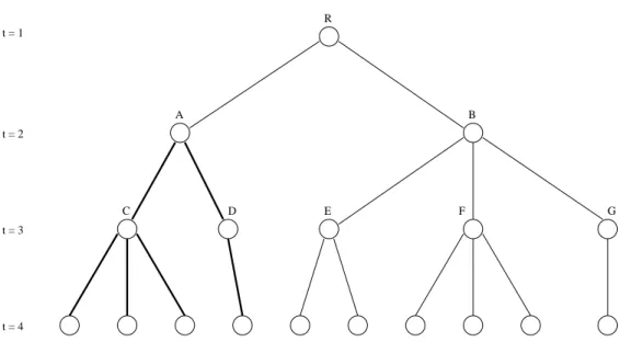
We illustrate our notation by applying it to the four-stage scenario tree in Figure 1. The root node R corresponds to the unique stage 1 realizationξ1. Table 1 gives examples of the history notation and the number of immediate descendants for nodes A, . . . ,G. The subtree with its root at node A is represented by Γ(ξ2,1) and its branches are darkened in Figure 1. The index set of the immediate
R
A B
C D E F G
t = 2 t = 1
t = 3
t = 4
Figure 1: An example of a four-stage scenario tree.
descendants of node B is D22 ={3,4,5}, and the corresponding stage 3 realizations are ξ33, ξ34, and ξ53. We haven2=n(1,1) = 2 andn3 =P2
r=1n(2, r) = 2 + 3 = 5. We refer to a generic node in the second stage, either A or B, byξ2, and a generic subtree rooted atξ2 by Γ(ξ2).
Table 1: Notation for the scenario tree in Figure 1
A B C D E F G
ξt,i ξ2,1 ξ2,2 ξ3,1 ξ3,2 ξ3,3 ξ3,4 ξ3,5
n(t, i) 2 3 3 1 2 3 1
By using the notation introduced, we can write (10)-(11), when {ξ˜t}Tt=1 has finite support, as follows:
minx1 c1x1+ X
k∈D11
pk|12 h1(x1, ξ2,k)
s.t. A1x1=b1 (14)
x1≥0,
where for allj= 1, . . . , nt, t= 2, . . . , T, ht−1(xt−1, ξt,j) = min
xt
cjtxt+ X
k∈Djt
pk|jt+1ht(xt, ξt+1,k)
s.t. Ajtxt=bjt−Btjxt−1 (15) xt≥0,
whereξt+1,k= (ξt,j, ξt+1k ),k∈Djt, and hT = 0. The conditional mass function is defined as pk|jt+1=P( ˜ξt+1=ξt+1k |ξ˜t=ξt,j), k∈Dtj,
and the stagetmarginal mass function ispit=P( ˜ξt=ξt,i),i= 1, . . . , nt. Note thatpj|iT+1= 0, ∀i, j.
We will use this formulation when we review the multi-stage L-shaped method in Section 2.3.
2.2 Sample Scenario Tree Construction
To construct a sample scenario tree, we perform the sampling in the following conditional fashion:
we begin by drawing n(1,1) = n2 observations of ˜ξ2 from F2(ξ2|ξ1) where ξ1 is the known first stage realization. Then, we form the descendants of each observationξ2,i, i= 1, . . . , n2, by drawing n(2, i) observations of ˜ξ3 fromF3(ξ3|ξ2,i). This process continues until we have sampledn(T −1, i) observations of ˜ξT from FT(ξT|ξT−1,i), i = 1, . . . , nT−1. The notation developed in Section 2.1 for a general finite scenario tree applies to a sample scenario tree. The number of descendants of a node ξt,i is now determined by the sample sizen(t, i). The total number of nodes in stage t+ 1 is nt+1 =Pnt
r=1n(t, r), and n(t) = |Dt| is the number of immediate descendants of a generic stage t node,ξt. The subtree associated with each descendant of nodeξt,i is Γ(ξt+1,j), j∈Dit.
In addition to the above structure for constructing a sample scenario tree, we require for the purposes of the estimators developed in Section 4 that the samples of ˜ξt+1be drawn fromFt+1(ξt+1|ξt) so that they satisfy the following unbiasedness condition
E[ft(xt,ξ˜t+1)|ξ˜t] =E[ 1 n(t)
X
i∈Dt
ft(xt,ξ˜t+1,i)|ξ˜t], (16)
wp1,t= 1, . . . , T−1. The simplest method for generating ˜ξt+1i , i∈Dt, to satisfy (16) is to require that they be (conditionally) independent and identically distributed (iid), but other methods, including some variance reduction schemes that have been used in stochastic programming (see, e.g., [1, 11, 26, 33, 40]), also satisfy (16).
Within the conditionally iid framework there are different types of sample scenario trees that can be generated. Consider the case when {ξ˜t}Tt=1 is interstage independent. One possibility is to generate a single set of iid observations of ˜ξt+1 and use this same set of descendants for all staget nodesξt,i, i= 1, . . . , nt. Another possibility is to generate mutually independent sets of staget+ 1
descendant nodes for all stage t nodes. We say the former method uses “common samples” and the latter “independent samples.” Both methods of generating a scenario tree satisfy (16). The independent-samples method introduces interstage dependency in the sample tree, which was not present in the original tree while the common-samples method preserves interstage independence.
Another advantage of the common-samples approach (relative to an independent-samples tree) is that the associated stochastic program lends itself to the solution procedures of [6, 16, 31, 46]. On the other hand, because of increased diversity in the sample, one might expect solutions under the independent-samples tree to have lower variability.
When using the common-samples approach the number of descendant nodes within each stage must be identical but the cardinality of Dt could vary with stage. In the independent-samples ap- proach, we have freedom to select different sample sizes at each node in the scenario tree. Dempster and Thompson [15] use the expected value of perfect information to guide sample tree construc- tion. Korapaty [38] and Chiralaksanakul [8] select the cardinality of descendant sets to reduce bias.
Provided that sampling is done in the conditional manner described above, with (16) satisfied, the methods we develop here can be applied to trees with non-constant sizes of descendant sets. That said, in our computation (Section 7) we restrict attention to uniform sample trees, i.e.,n(t, i) =|Dti| is constant for alliandt.
Given an empirical, i.e., sampled, scenario tree an approximating problem for (7)-(9) can be stated as
ˆ
z∗ = min
x1
1 n(1,1)
X
i∈D11
fˆ1(x1,ξ˜1,Γ( ˜ξ2,i)) (17)
where
fˆt−1(xt−1,ξ˜t−1,Γ( ˜ξt,j)) = min
xt
1 n(t, j)
X
i∈Dtj
fˆt(xt−1, xt,ξ˜t,j,Γ( ˜ξt+1,i)), (18)
ξ˜t,j = ( ˜ξt−1,ξ˜tj),j∈Dt−1, t= 2, . . . , T−1, and
fˆT−1(xT−1,ξ˜T−1,Γ( ˜ξT ,j)) = fT−1(xT−1,ξ˜T ,j) (19)
= min
xT
fT(xT−1, xT,ξ˜T ,j),
ξ˜T ,j = ( ˜ξT−1,ξ˜Tj), j ∈ DT−1. The value function at a stage t node ξt depends on the stochastic history (known at timet), ˜ξt=ξt, the associated decision history,xt, and the sample subtree Γ(ξt).
In going from (7)-(9) to (17)-(19), we are approximating the original population scenario tree by a sample scenario tree.
One of the policy-generation methods we develop is for multi-stage stochastic linear programs and
so we explicitly state the associated approximating problem of (10)-(11):
minx1 c1x1+ 1 n(1,1)
X
k∈D11
ˆh1(x1,ξ˜1,Γ( ˜ξ2,k))
s.t. A1x1=b1 (20)
x1≥0, where for allj= 1, . . . , nt, t= 2, . . . , T,
ˆht−1(xt−1,ξ˜t−1,Γ( ˜ξt,j)) = min
xt
cjtxt+ 1 n(t, j)
X
k∈Djt
ˆht(xt,ξ˜t,j,Γ( ˜ξt+1,k))
s.t. Ajtxt=bjt−Btjxt−1 (21) xt≥0,
ξ˜t,j = ( ˜ξt−1,ξ˜tj) and ˆhT ≡0.
2.3 The Multi-stage L-shaped Method
In this section we briefly review the multi-stage version of the L-shaped method. The method was originally developed by Van Slyke and Wets [54] for two-stage stochastic linear programs, and was later extended to multi-stage programs by Birge [2]. It is an effective solution method for such problems [20, 51] and plays a central role in the policy generation procedure we discuss in Section 3.1. The multi-stage L-shaped method decomposes (14)-(15) by stage and then separates stage-wise problems by scenario to achieve a subproblem at each nodeξt,i, denoted sub(t, i),i= 1, . . . , nt, t= 1, . . . , T−1, of the following form:
min
xt,θt
citxt+ θt
s.t. Aitxt = bit−Btixa(i)t−1 :πt (22)
−G~itxt+e θt ≥ ~gti :αt
xt ≥ 0.
The rows of the matrixG~itcontain cut gradients; the elements of the vector~gtiare cut intercepts; and, eis the vector of all 1’s. πt andαt are dual row vectors associated with each set of constraints. For t=T, the subproblems are similar to (22) except that there are no cut constraints and no variable θT. To compute the cut gradient and intercept in sub(t, i), all the descendants of sub(t, i) are solved at a given stagetdecision,xt, to obtain (πt+1j , αjt+1), j∈Dti. Then, the cut gradient is
Git=− X
j∈Dti
pj|it+1πt+1j Bt+1j , (23)
and the cut intercept is
git= X
j∈Dti
pj|it+1πt+1j bjt+1+ X
j∈Dti
pj|it+1αjt+1~gt+1j , (24) where the second term on the right-hand side of (24) is absent ift=T−1. For sub(t, i), the rows of the matrixG~itare composed of the cut gradient row vectors,Git, and the components of the vector~gti are composed of the cut intercepts,gti. An algorithmic statement of the multi-stage L-shaped method using the so-called fastpass tree traversal strategy is given in Figure 2. In the fastpass strategy, an optimal solution from each subproblem is passed to its descendants until the last stage is reached, and then the cuts formed by the descendants at each stage are passed back up to the corresponding ancestor subproblems. Other tree-traversal strategies are also possible but empirical evidence appears to support the use of the fastpass strategy [25, 43, 58].
Step 0 Definetoler≥0 and letz=∞.
Initialize the set of cuts for sub(t, i) withθt≥ −M, i= 1, . . . , nt, fort= 1, . . . , T−1. (M sufficiently large.) Step 1 Solve sub(1,1) and let (x1, θ1) be its solution.
Letz=c1x1+θ1. Step 2 Dot= 2 toT
Doi= 1, . . . , nt
Form the right-hand side of sub(t, i): bit−Bitxa(i)t−1. Solve sub(t, i). Letxitbe its solution.
Ift=T, letπiT be the optimal dual vector.
Let ˆz=c1x1+PT t=2
Pnt i=1pitcitxit.
Step 3 If ˆz < zthen letz= ˆzandxi,∗t =xit,∀i, t.
Ifz−z≤min(|z|,|z|)·tolerthen stop: xi,∗t ,∀i, tis a policy with objective function value within 100·toler% of optimal.
Step 4 Dot=T−1 downto 2 Doi= 1, . . . , nt
Form (Git, git).
Augment sub(t, i)’s set of cuts with−Gitxt+θt≥git. Form the right-hand side of sub(t, i): bit−Bitxa(i)t−1. Solve sub(t, i). Let (πit, αit) be the optimal dual vector.
Form (G11, g11).
Augment sub(1,1)’s set of cuts with−G11x1+θ1≥g11. Goto Step 1.
Figure 2: The multi-stage L-shaped algorithm using the fastpass tree traversal strategy for aT-stage stochastic linear program.
3 Two Policy Generation Methods
3.1 Linear Problems with Interstage Independence
In this section, we develop a procedure to generate a feasible policy for the multi-stage stochastic linear program (14)-(15) when {ξ˜t}Tt=1 is interstage independent. Our method works as follows:
First, we construct a sample scenario tree, denoted Γc, using the common-samples method described in Section 2.2. Then, the instance of (20)-(21) associated with Γc is solved with the multi-stage L-shaped algorithm of Figure 2 (the “c” subscript on Γ stands for “cuts”). When the algorithm stops, we obtain a policy whose expected cost is within 100·toler% of optimal for (20)-(21). We now describe how we use this solution to obtain a policy for the “true” problem (10)-(11).
When the algorithm of Figure 2 terminates, each sub(t, i) contains the set of cut constraints generated during the solution procedure. Since Γc is constructed with the common-samples scheme, the sample subtrees rooted at the stage t nodes are all identical, i.e., the sample scenario tree Γc exhibits interstage independence. Thus, the cuts generated for a stagetnode are valid for all other nodes in stage t. We will use the collection of cuts at each stage to construct a policy to problem (10)-(11).
Let G~it,c and~gt,ci denote the cut-gradient matrix and cut-intercept vector for sub(t, i) when the multi-stage L-shaped method terminates. Then, we define a stage t optimization problem used to generate the policy for (10)-(11) as follows:
minxt ctxt+θt
s.t. Atxt=bt−Btxt−1 (25)
−G~it,cxt+e θt≥~gt,ci , i= 1, . . . , nt xt≥0,
fort = 2, . . . , T. Fort = 1, (25) does not contain the termB1x0 in the first set of constraints, and fort=T the cut constraints are absent. A policy must specify what decision, ˆxt(ξt), to take at each stagetfor a givenξt. Our policy computes ˆxt(ξt) by solving (25) with (At, Bt, bt, ct) specified byξt, and withxt−1 determined by having already solved (25) under subvectors ofξtcorresponding to the preceding stages. Such a policy is nonanticipative because when solving (25) the process{ξ˜t}Tt=1 is known only through staget. Relatively complete recourse ensures that ˆxt(ξt) will lead to a feasible decision in stages t+ 1, . . . , T. The superscript on the cut-gradient matrix and the cut-intercept vector in (25) denotes the index of the stage t node in Γc from which we obtain the cuts, andnt is the total number of stage tnodes in Γc. So, if sub(t, i) in Γc hasKti cuts then the total number of cuts in (25) isPnt
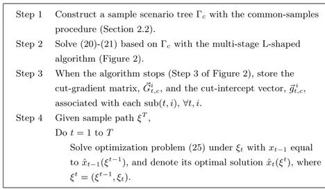
i=1Kti. We refer to this procedure asP1 and summarize it in Figure 3.
The solution procedure, as we have described it above, is a naive version of the multi-stage L- shaped method because it stores a separate set of cuts at each sub(t, i) when solving (20)-(21) under
Step 1 Construct a sample scenario tree Γcwith the common-samples procedure (Section 2.2).
Step 2 Solve (20)-(21) based on Γcwith the multi-stage L-shaped algorithm (Figure 2).
Step 3 When the algorithm stops (Step 3 of Figure 2), store the cut-gradient matrix,G~it,c, and the cut-intercept vector,~gt,ci , associated with each sub(t, i),∀t, i.
Step 4 Given sample pathξT, Dot= 1 toT
Solve optimization problem (25) underξtwithxt−1 equal to ˆxt−1(ξt−1), and denote its optimal solution ˆxt(ξt), where ξt= (ξt−1, ξt).
Figure 3: Procedure P1 to generate a feasible policy for a T-stage stochastic linear program with relatively complete recourse when{ξ˜t}Tt=1 is interstage independent.
Γc. Because Γc is interstage independent, we instead store a single set of cuts at each stage. This speeds the solution process and aids in eliminating redundant cuts when forming (25).
We have described the method for generating cuts at each stage by solving (20)-(21) under Γc
exactly (or within 100·toler%) using the algorithm of Figure 2. However, this may be computationally expensive to carry out if Γc is large. If T is large but the number of descendants at each stage t node is “manageable” then we could instead employ one of the sampling-based algorithms designed for such problems [6, 16, 31, 46].
Procedure P1 exploits convexity and interstage independence to generate feasible policies. In- terstage independence plays a key role since the set of cuts generated as an approximation to E[ht(xt,ξ˜t+1)|ξ˜t = ξt] can also be used for E[ht(xt,ξ˜t+1)|ξ˜t = ξ0t] when ξt 6= ξ0t because these two functions are identical. GeneralizingP1to handle problems with interstage dependency requires specifying how to adapt, or modify, cuts generated for E[ht(xt,ξ˜t+1)|ξ˜t =ξt] to another cost-to-go function conditioned on ˜ξt =ξ0t. For general types of dependency structures, this may be difficult (and so we develop a different approach in the next section). However, such adaptations of cuts are possible in the special case where {ξ˜t}Tt=1 consists of {(˜ct,A˜t,B˜t,η˜t)}Tt=1, which is interstage independent and{˜bt}Tt=1 has the following dependency structure:
˜bt=
t−1
X
j=1
(Rtj˜bj+Sjtη˜j) + ˜ηt, t= 2, . . . , T. (26) Here, Rtj and Stj are given deterministic matrices with appropriate dimensions. Series (26) is a
[53]. With this probabilistic structure, Infanger and Morton [35] derive cut sharing formulae to be used in the L-shaped method. These results can be applied to modify Step 3 and 4 ofP1. In Step 3, we store scenario-independent cut information, i.e., cut gradients, independent cut intercepts, and so- called cumulative expected dual vectors (see [35]) obtained from the multi-stage L-shaped algorithm in Step 2. Then, in Step 4, for a givenξt, scenario-dependent cuts in (25) can be computed using the analytical formulae of [35, Theorem 3].
3.2 Problems with Interstage Dependence
The method of Section 3.1 handles stochastic linear programs with interstage independence, or a special type of dependence. In this section, we propose a different approach, which is computationally more demanding but allows for nonconvex problems with relatively complete recourse and general interstage dependency structures. In particular we consider the general T-stage stochastic program defined by (7)-(9) under assumptions (A1)-(A4) given in Section 2.1.
Our feasible policy construction for (7)-(9) works as follows: For a given ξt, we obtain ˆxt(ξt) by solving an approximating problem (from staget toT) based on an independently-generated sample subtree, denoted Γr(ξt) (the “r” subscript stands for “rolling”). Specifically, for a given ξt and xt−1, Γr(ξt) is constructed by the conditional sampling procedure described in Section 2.2 (either the common-samples or independent-samples method can be used). Then, ˆxt(ξt) is defined as an optimal solution of
minxt
1 n(t)
X
i∈Dt
fˆt(xt−1, xt,Γr( ˜ξt+1,i)), (27) where
fˆτ−1(xτ−1,ξ˜τ−1,Γr( ˜ξτ,j)) = min
xτ
1 n(τ, j)
X
i∈Djτ
fˆτ(xτ−1, xτ,ξ˜τ,j,Γr( ˜ξτ+1,i)), ξ˜τ,j= ( ˜ξτ−1,ξ˜τj),j ∈Dτ−1, τ =t+ 1, . . . , T−1, and
fˆT−1(xT−1,ξ˜T−1,Γr( ˜ξT ,j)) = min
xT fT(xT−1, xT,ξ˜T ,j), ξ˜T ,j= ( ˜ξT−1,ξ˜Tj),j ∈DT−1.
Our policy, which computes ˆxt(ξt) by solving (27), is nonanticipative. None of the decisions made at descendant nodes in stagest+ 1, . . . , T, are part of the policy. Decisions in these subsequent stages (e.g.,t+ 1) are found by solving another approximating problem (e.g., from staget+ 1 toT) with an independently-generated sample tree. Similarly, the decisions at previous stages needed to findxt−1 are also computed using independently-generated sample trees. Relatively complete recourse ensures that ˆxt(ξt) will lead to feasible solutions in stages t+ 1, . . . , T. We denote this policy-generation procedure byP2 and summarize it in Figure 4. AlthoughP2 is applicable to a more general class of stochastic programs thanP1, we still need a viable solution procedure to solve (27). In a non-convex instance of (27), finding an optimal solution can be computationally difficult.
Given sample pathξT, Dot= 1 toT
Independently construct a sample subtree Γr(ξt).
Solve approximating problem (27) withxt−1equal to ˆ
xt−1(ξt−1), and denote its optimal solution ˆxt(ξt), where ξt= (ξt−1, ξt).
Figure 4: ProcedureP2to generate a feasible policy for aT-stage stochastic program with relatively complete recourse.
4 Policy Cost Estimation
Under scenario ˜ξT, the cost of using a given feasible policy, ˆxT( ˜ξT), in (7)-(9) isfT(ˆxT( ˜ξT),ξ˜T), and EfT(ˆxT( ˜ξT),ξ˜T)≥z∗ because this is a feasible, but not necessarily optimal, policy. In general, it is impossible to compute this expectation exactly. In this section, we describe a scenario-based method and a tree-based method to estimateEfT(ˆxT( ˜ξT),ξ˜T). These estimation procedures can be carried out for any feasible policy but, when appropriate, we discuss specific issues for policiesP1 andP2.
4.1 Scenario-based Estimator
When employing a policy under scenarioξT, we obtain a sequence of feasible solutions, ˆx1(ξ1), . . . , ˆ
xT(ξT) (see Figures 3 and 4 for policies P1 and P2). The cost under scenarioξT is then given by fT(ˆxT(ξT), ξT). In the case of aT-stage stochastic linear program, this cost is
fT(ˆxT(ξT), ξT) =
T
X
t=1
ct(ξt)ˆxt(ξt). (28)
Again, we emphasize that with both P1 and P2, ˆxT(ξT) is nonanticipative because when we carry out the procedures of Figures 3 and 4 to find ˆxt(ξt) the subsequent realizations,ξt+1, . . . , ξT, are not used (in fact, they need not even be generated yet).
In order to form a point estimate ofEfT(ˆxT( ˜ξT),ξ˜T) whose error can be quantified, we generate ν iid observations of ˜ξT, ˜ξT ,i, i = 1, . . . , ν. To form each ˜ξT ,i, observations of ˜ξt are sequentially drawn from the conditional distributionFt(ξt|ξt−1,i), t= 2, . . . , T. Then, the sample mean estimator is
U¯ν = 1 ν
ν
X
i=1
fT(ˆxT( ˜ξT ,i),ξ˜T ,i). (29) LetSu2 be the standard sample variance estimator of varfT(ˆxT( ˜ξT),ξ˜T). Then,
P
Ef (ˆxT( ˜ξT),ξ˜T)≤U¯ +t Su
√
= P
√
ν( ¯Uν−EU¯ν)
≥ −t
,
where tν−1,α denotes the (1−α)-level quantile of a Student’st random variable withν−1 degrees of freedom. By the central limit theorem for iid random variables,
ν→∞lim P √
ν( ¯Uν−EU¯ν)
Su ≥ −tν−1,α
= 1−α.
Hence, for sufficiently large ν, we infer an approximate one-sided 100·(1−α)% confidence interval forEfT(ˆxT( ˜ξT),ξ˜T) =EU¯ν of the form − ∞,U¯ν+tν−1,αSu/√
ν .
4.2 Tree-based Estimator
The scenario-based estimation procedure of the previous section generatesν iid observations of ˜ξT. The estimation procedure in this section is instead based on generatingν iid sample scenario trees.
Later, in Section 5, we turn to estimating a lower bound onz∗. That lower bound is based on sample scenario trees and can be combined with either the scenario- or tree-based estimators to establish the quality of a solution policy. As will become apparent, the tree-based estimator in this section can be coupled with the lower-bound estimator in a manner not possible for the scenario-based estimator.
Let Γ be a sample scenario tree generated according to the conditional sampling framework of Section 2.2, and letnT be the number of leaf nodes. Then, Γ may be viewed as a collection of scenarios, ξ˜T ,j, j = 1, . . . , nT, which are identically distributed but are not independent. An unbiased point estimate ofEfT(ˆxT( ˜ξT),ξ˜T) is given by
W = 1
nT nT
X
j=1
fT(ˆxT(ξT ,j), ξT ,j). (30)
The numerical evaluation of fT(ˆxT(ξT ,j), ξT ,j), j = 1, . . . , nT, under a specific policy occurs in the manner described in Section 4.1.
To quantify the error associated with the point estimate in (30), we generate ν iid sample trees, Γi, i= 1, . . . , ν. Each of these trees is constructed according to the procedure described in Section 2.2 (again, under either the common-samples or independent-samples procedure). The number of sce- narios in each Γi is again nT, and the scenarios of Γi are ξT ,ij, j = 1, . . . , nT. The point estimate under Γi is
Wi= 1 nT
nT
X
j=1
fT(ˆxT( ˜ξT ,ij),ξ˜T ,ij). (31) By construction,Wi, i= 1, . . . , ν, are iid. So,
W¯ν = 1 ν
ν
X
i=1
Wi
is the tree-based point estimate ofEfT(ˆxT( ˜ξT),ξ˜T). LetS2wbe the standard sample variance estima- tor of varW. BecauseEW¯ν=EW =EfT(ˆxT( ˜ξT),ξ˜T), a confidence interval under the tree-based ap-
proach is constructed in a similar manner as in the scenario-based case, i.e., −∞,W¯ν+tν−1,αSw/√ ν is an approximate one-sided 100·(1−α)% confidence interval for EfT(ˆxT( ˜ξT),ξ˜T).
5 Lower Bound Estimation
In this section, we develop a statistical lower bound forz∗, the optimal value of (7)-(9), and describe how to use this estimator to construct a one-sided confidence interval onz∗. Again, the motivation for forming such a confidence interval is to couple it with one of the confidence intervals from the previous section in order to establish the quality of a feasible policy, including those generated byP1
andP2. Here, quality is measured via the optimality gap of a policy defined asEfT(ˆxT( ˜ξT),ξ˜T)−z∗. Our lower-bound estimator requires little structure on the underlying problem, and we derive it using the notation of Section 2.1. First, we state the lower bound result for (7) whenT = 2 in Lemma 1 (see also [42, 45]). In this case, (7) becomes a two-stage stochastic program with recourse, and the approximating problem, (17)-(19), reduces to
ˆ
z∗= min
x1
1 n2
n2
X
i=1
f1(x1,ξ˜2,i), (32)
where
f1(x1,ξ˜2,i) = min
x2 f2(x1, x2,ξ˜2,i), fori= 1, . . . , n2.
Lemma 1. Assume X1(ξ1)6=∅ and is compact, f2(x1,·,ξ˜2) is lower semi-continuous, wp1, for all x1 ∈X1(ξ1), and E
infx2f2(x1, x2,ξ˜2)
<∞ for all x1 ∈ X1(ξ1). Let z∗ be defined as in program (7) with T = 2andzˆ∗ be defined as in program (32). If ξ˜2,1, . . . ,ξ˜2,n2 satisfy
Eh
f1(x1,ξ˜2)i
=E
"
1 n2
n2
X
i=1
f1(x1,ξ˜2,i)
# ,
i.e., condition (16) witht= 1, then
z∗≥Ezˆ∗.
Proof. The lower semi-continuous and finite expectation assumptions onf2ensure that the objective functions of (7) and (32) are lower semi-continuous, and hence both have finite optimal solutions achieved on X1(ξ1). The lower bound is then obtained by exchanging the order of expectation and