322.061: Fundamentals of Numerical Thermo-Fluid Dynamics Exercise 4
Computed domain
x0 x1 x2 x3 xN
−2 xN−1 xN xN+1
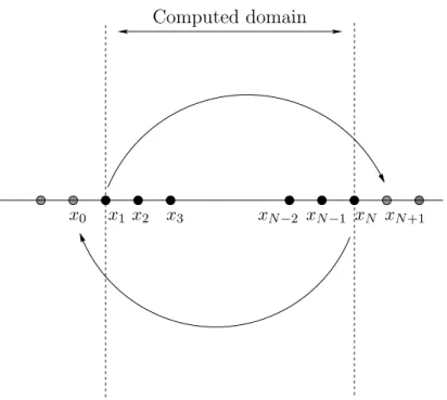
Figure 1: Schema of a periodic BC.
In numerical methods it is often useful to provide periodic boundary conditions on your system such that one can observe some characteristics of the scheme. The main idea of the periodic boundary condition is to say that ”what comes out from one side, comes in from the other side of the domain”.
Let us consider a field U that is discretized, on the domain of fig. 1. U(x1) will be equal t U(xN+1), and a value that is in U(xN) will also be inU(x0), and conversely.
This kind of boundary condition allows for instance the modelling of a wave through an potentially infinite domain, without having to compute the points in all the domain.
Let us say that the size of the domain Ω = [x1, xN] on which we will compute the solution is discretized in N values. Moreover, one uses the following scheme for a time evolution ;
Uin+1 =c Ui−1n +a Uin+b Ui+1n (1) To apply the periodic BC, we say that :
• atx1, U1n+1 =c UNn +a U1n+b U2n
• atxN, U1n+1 =c UNn−1+a UNn +b U1n
The matrix associated to this discretized problem is then :
A=
a b · · · 0 · · · c
c a b 0
. .. ... ...
. .. ... ...
. .. ... b
b · · · 0 · · · c a
(2)
1