Dissertation Imagingofmagnetizationdynamicsintemperaturegradients

Imaging of magnetization dynamics in temperature gradients

Dissertation

zur Erlangung des Doktorgrades der Naturwissenschaften (Dr. rer. nat.)

der Fakult¨at f¨ur Physik der Universit¨at Regensburg

vorgelegt von

Michael Vogel

aus Kaiserslautern

im Jahr 2018

Promotionsgesuch eingereicht am: 1. Februar 2017

Die Arbeit wurde angeleitet von: Prof. Dr. Christian H. Back

Contents

1 Overview 7

I Theoretical and Experimental Background 11

2 Theoretical Background 12

2.1 Magnetic Vortex Core . . . 12

2.2 Micromagnetic Simulations and Thiele Equation . . . 16

2.3 Extended Thiele Equation for Vortex Core Motion . . . 24

2.4 Extended Thiele Equation for Coupled Vortices . . . 37

3 Magnetic Imaging 43 3.1 Introduction . . . 43

3.2 Lorentz Microscopy . . . 45

3.3 STXM . . . 51

4 Sample Preparation 56 4.1 Materials . . . 56

4.2 Litography . . . 60

5 Designing the 2D temperature landscape 67 5.1 Thermal modelling (COMSOL) . . . 67

5.2 Generating high temperature gradients on a SiN-membrane . . . 69

5.3 Heating a single disk in a pair of coupled vortex oscillators . . . 71

II Results 73 6 Fine-grain phase control in magnetic vortex oscillators networks for neuromorphic computing 74 6.1 Frequency spectra of a pair of coupled vortex oscillators . . . 76

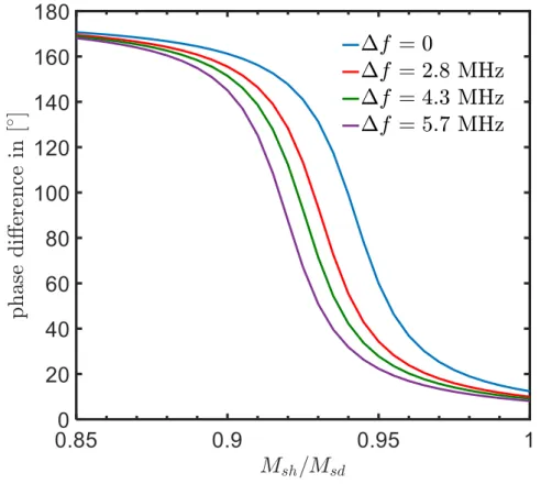
6.2 Phase manipulation in a pair of coupled vortex oscillators . . . 78

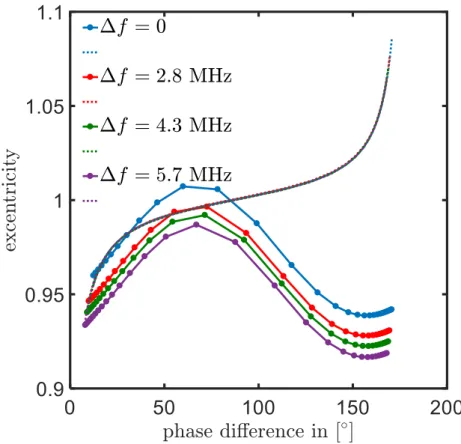
6.3 Dependence of the eccentricity on phase difference . . . 80

7 Vortex Core Motion driven by Magnon Spin Seebeck Effect 81 7.1 Observation of vortex core movement due to thermomagnonic spin

torques by Lorentz TEM measurements . . . 83 7.2 Statistic investigation of the movement due to thermomagnonic spin

torques . . . 84 7.3 Comparison of the movement due to spin transfer torque induced

by thermal generated magnons and direct electric currents . . . 87

8 Summary / Outlook 89

9 Appendix 90

9.1 Material parameters . . . 90 9.2 Scaling behaviour of vortex core motion dependent on the magnon

velocity . . . 91

Acknowledgements

First of all I am grateful to my supervisor Prof. Dr. Christian H. Back for the support during the experimental and theoretical challenges in the making of this thesis and the opportunity to carry out my PhD degree in his group. I have greatly benefitted from the collaboration with him and all the members of his group and from his inputs and encouragements. I extend my gratitude to Prof. Dr. Josef Zweck for enabling the TEM measurements carried out during the making of the thesis and for sharing his knowledge on microscopy and optics.

My sincere thanks also goes to the members of the dissertation committee, Prof.

Dr. G. Bali, Prof. Dr. J. Repp and Prof. Dr. D. Bougeard for their time and patience.

In my work on the theoretical modelling of the experiments presented here I have received a lot of input from Prof. Dr. Claudia Mewes and Prof. Dr. Tim Mewes, especially on the micromagnetic simulations, using the micromagnetics code M

developed by them. Further their input on developing the analytic framework using an Extended Thiele equation model was of invaluable importance.

Special thanks goes to Dr. Hermann Stoll, Dr. Markus Weigand and Michael Bechtel from the MPI Stuttgart for technical support during the measurements at BESSY II around the clock.

I would like to offer my special thanks to Prof. Dr. Stuart Parkin for allowing me to visit his labs at IBM Almanden.

I am grateful to Prof. Dr. Guenther Reiss and Prof. Dr. Andy Thomas for providing sputtered thin films.

I am especially thankful to Prof. Dr. Dieter Weiss and his entire group for providing infrastructure in the clean-room for sample preparation and characteri- zation.

I thank Dr. Jean-Yves Chauleau, Dr. Matthias Kronseder and Dr. Lin Chen for fruitful discussions and the collaboration on different projects not presented here.

Further my thank goes to my colleagues from my department that contributed in

the making of this thesis. Here I want to emphasize the help of Johannes Wild and

Felix Schwarzhuber who spent a lot of measurement time with me at the TEM.

I have also had support from Bernhard Zimmermann who helped charaterizing temperature gradients in small nanostructures in the making of his bachelor thesis.

I also enjoyed working with him on FMR measurements on coupled magnetic bi- layer system in out of plane temperature gradients (not shown here) and spending time with him at BESSY. I thank Ajay Gangwar for valuable insights on preparing samples on SiN-membranes.

I also want to thank my coauthors and callaborators on different projects not shown in this thesis. Martin Decker ( spin orbit induced switching), Johannes Stigloher (TR-MOKE measurements on the manipulation of spin waves by an applied temperature gradient), Maximilian Schmid (Transverse Spin Seebeck Ef- fect measurements that turned out to be Planar Nernst Effect measurements) and Sasmita Srichandan (Electrical and thermal transport coefficients of CoFe thin films). Many thanks go to the Master students I had the opportunity to work with, namely Michael Mueller and Susanne Brunner. Apart from those already mentioned I want to thank all the other members from the department who let me enjoy my time in Regensburg, especially Robert Islinger and Tobias Weindler.

I can not thank enough our secretaries Magdalena Pfleger, Doris Meier, Sylvia Hrdina, Claudia Zange and our technician Markus Hollnberger.

Last but not least, I thank my niece Marie for mental support. My deepest gratitude goes to my wife Alexandra for all the support during my time as a PhD student in Regensburg and proof-reading this thesis with her special powers. I am forever thankful to my mother Maria for granting me such freedom to choose my path and always encouraging me.

Part of this work was supported by the DFG SPP 1548.

Overview 1

Neuromorphic computing describes the use of very-large scale integrated logic (VLSI) systems to mimic neurobiological architectures [1] promising advances in computation density and energy efficiency [2] in the post Moore’s law age of com- puting [2, 3]. In nature neurons behave as nonlinear oscillators developing rhyth- mic activity and interact to process information [4]. Hence, oscillatory neural networks (ONNs) are promising building blocks for VLSIs, harnessing either the frequency or phase as state variable for logic operations [5–7]. Recently, a novel approach using nanoscale spintronic-oscillators in the form of magnetic tunnel junctions [8, 9] has been experimentally demonstrated to realize such VLSIs [10].

Two key requirements for oscillators used in VLSIs are high stability to process information reliable and the possibility to stack the oscillators in high density ar- rays. In order to stack the total number of neurons in the human brain ≈ 10

[11]

in an ONN on a 10 cm by 10 cm chip, the size of the single elements have to be of the order of 100 nm. A possible spintronic building block for such networks are magnetic vortex oscillators as investigated in this thesis. The magnetic vortex structure [12, 13] is characterized by an in plane curling magnetization, the sense of rotation defining the chirality c = ± 1, and a perpendicular magnetized core at the center who’s direction defines the polarity p = ± 1. For disk shaped magnetic elements this magnetization structure causes flux closure of the in plane magneti- zation with the out of plane core with a size of 10 nm to 30 nm generating a small stray field [14]. The flux closure configuration causes a highly stable ground state configuration and allows for closed stacked arrays due to almost no interaction.

Their lateral size is scalable from nm size to a few µm and is accompanied by

dynamics from the kHz to the GHz regime [15]. In the low frequency excitation

state, called the gyration mode [12, 14], surface magnetic charges appear, which allow dynamic dipolar interaction in a pair of vortices next to each other [16, 17].

cold hot

V_- V_~

Figure 1.1: Sketch of Experiment 1: In a pair of stray field coupled magnetic vortex oscillators the disk on the right is excited by an ac charge current via STT, the disk on the left is heated to control the resonance frequency via a change of the saturation magnetization. This allows the control of the phase relation between the two excitations (white ellipses).

In the first experiment presented in this thesis a pair of stray field coupled mag- netic vortex oscillators (see fig. 1.1) is investigated by Lorentz Transmission Elec- tron Microscopy (L-TEM) and Scanning Transmission X-ray Microscopy (STXM).

One of the oscillators is excited by an ac current via the Spin Transfer Torque (STT) effect. The second oscillator is heated via Joule heating, thereby reducing the saturation magnetization and causing a shift of the relative phase relation of the two oscillators to arbitrary values between the in phase and out of phase state (fine-grain phase control). Phase manipulation in a controlled manner is critical in ONNs and promises a wide range of applications from mimicking rhythmic motive patterns in robotics [18, 19] to neuromorphic image recognition [20].

The second experiment investigates the manipulation of the vortex core position

by pure thermomagnonic torques. Traditionally the manipulation of topological

solitons such as magnetic vortices and skyrmions is achieved by spin polarized

electric charge currents due to the application of an electrical potential [21]. As

recently proposed by theory, thermally excited magnons created by temperature

gradients can also be used to manipulate magnetic structures [22, 23]. Here the

theoretically well understood dynamics of magnetic vortex cores, when subject to

thermal gradients, is investigated. Transmission Electron Microscopy measure-

ments on magnetic vortices in temperature gradients created by local static Joule

Figure 1.2: Sketch of Experiment 2: A magnetic vortex core inside a Py disk is placed next to a meander type heater. The temperature of the heater is increased by Joule heating. The Py disk sits on the edge of a SiN-membrane. The frame of the membrane doubles as heatsink. The movement of the core is investigated by L-TEM measurements.

heating (see fig. 1.2) were performed. A large deflection compared to electric spin

transfer torque excitation of the magnetic vortex core is observed. It is shown

that the magnitude of the deflection depends on the applied heating power and

the polarization of the core. To analyze the experimental results, a generalized

Thiele equation [24] model, including the different forces acting on the vortex core

due to the applied temperature gradient, was developed. This analysis allows

the estimation of the magnitude of the core motion for the involved force terms

and therefore the differentiation of the origin of the experimental observed vortex

movement.

Part I

Theoretical and Experimental

Background

Theoretical Background 2

2.1 Magnetic Vortex Core

Figure 2.1: Micromagnetic simulation of relaxed magnetic vortex core. Color indicating the direction of the curling in plane magnetization. The out of plane core in the center points in upward direction.

Vortices are topological solitons [25] occurring in many classical field theories.

They are stable topologically protected quasi-particles with finite mass and smooth

structures [25]. In physical dynamic systems vortex like structures exist across a

wide range of length scales from quantized vortices in superconductors [25] at inter atomic length-scales to galactic structures with dimensions of several kpc (1 kpc ≈ 3 × 10

m )[26]. Their dynamic is often governed by similar non linear differential equations. The magnetic vortex structure fig. 2.1 is characterized by an in-plane curling magnetization and a perpendicularly magnetized core at the center [12, 13]. The sense of rotation determines the chirality c = ± 1. The direction of the perpendicular core defines the polarity p = ± 1 which is one of a total of two topological charges of a magnetic vortex core, the other one being the vorticity v = 1, which all vortex structures have in common.

p = +1 c = +1

p = -1 c = +1

p = +1 c = -1

p = -1 c = -1

Figure 2.2: Possible combinations of

and

,

: height information

,M

: color coded.

The possible combination of p and c allow for a total of four logical states (see section 2.1) for information processing. The magnetic vor- tex is one of the elementary magnetic ground states found in lateral confined magnetic thin films [27]. Due to it’s topological protection [28]

and low stray fields the magnetic vortex state is magnetically very stable. For disk shaped mag- netic elements this configuration causes flux closure in the in-plane magnetization, with only the out of plane core with a typical size of 10 nm to 30 nm [29] generating a small stray field. The vortex ground state has a complex spin excita- tion spectrum, with a low-frequency mode of displacement of the vortex as a whole called the gyration mode [13, 14]. Magnetization dynamics in this case can be well described within the framework of micro-magnetic simulations and an analytic solution based on the Thiele equation (section 2.2). The resonance frequency f

of the gyration mode scales with the lateral size of the magnetic disk and the thick- ness (see fig. 2.9) allowing scalable dynamics in the kHz to GHz regime [15]. The vortex gyration can be excited by different means. Traditionally the excitation is done non-locally by low ( ≈ mT) in plane magnetic field pulses [30]. It is also possible to locally excite the core by application of a spin polarized current [31].

This manipulation of the magnetization dynamics at the nanoscale by the means of electric currents has become one of the most attractive subjects in the field of magnetic vortex core dynamics from both the fundamental and the application viewpoints [31, 32].

In the low frequency excitation state surface magnetic charges appear due to

the core displacement [13]. In case of a pair of vortices next to each other (see

fig. 2.4), this brings about dynamic dipolar interaction between them [16, 17]

t[ns] 0 54.4 109 163 217 150 nm

Figure 2.3: Time resolved STXM measurement of a excited vortex core in the gyration mode. The vortex core is excited by short current pulses at a resonance frequency of

= 240 MHz. The time-resolution of the measurement is 66 ps. The spot is tracked via image recognition and the positions are shown in white. 5 frames at equidistant time-steps are shown here.

(see section 2.4). This opens a manifold of possibilities. Due to their coupling magnetic vortex oscillators can be used as building blocks for oscillatory networks.

So far many implementations of this have been proposed. The signal transfer across a chain of such oscillators has been studied [33, 34] oberserving wave modes travelling through such artificial crystals. Basic building blocks for computation and logic manipulation have been realised, such as XOR and OR operators [35]

as well as transistors [36]. In chapter 6 a new method to realise fine-grain phase control in such networks is demonstrated.

200 nm

Figure 2.4: L-TEM image of the pair of magnetic vortex oscillators with a radius of

= 0.9 µm. The gyration mode is driven by a cw excitation at 240 MHz applied on the left disk. The gyration mode can be seen at the middle of both disks in form of ellipses.

These oscillatory applications harness resonant excitation of the vortex core eas-

ily increasing the static elongation of the vortex core by a factor of 1000. So far the

only means to image the elongated vortex core by static excitation have been large

external magnetic fields [37] (see fig. 2.5). Even though STT by spin polarized

currents is a very effective way to manipulate magnetization dynamics [38] with

many applications from racetrack memory [38] to STT-MRAM predicted to out- perform current memory technologies in the near future [38], the required current densities for Py would be magnitudes of order larger than the destruction thresh- old to experimentally observe a movement of the vortex core (see section 2.3).

In this work a new way to manipulate the magnetic vortex core structure by the Magnon Spin Seebeck Effect (see section 2.3 and chapter 7) is presented resulting in movement 5 order of magnitude larger than possible via spin polarized electric currents.

a) b)

c)

Figure 2.5: L-TEM measurement of 20 nm thick Py disks with a radius of 1 µm a) In a

zero in-plane magnetic field the vortex core is at the center of the Py disk. b) After a

field sweep up to 30 000 A

m the vortex core is pushed to the edge of the Py disk. c) The

path traveled by the vortex core differs from a straight line and indicates the influence of

the local energy landscape created by defects in the SiN-membrane (see section 4.1.1).

2.2 Micromagnetic Simulations and Thiele Equation

The magnetization dynamics of the spin core motion driven by a spin polarized cur- rent is phenomenological well described by the extended Landau-Lifshitz-Gilbert equation [39]:

d − → M

dt = − γ − → M × − →

H

+ α M

− →

M × d − → M dt

− 1

M

M ~ × ( M ~ × ( b

~j · − →

∇ ) M ~ ) − ξ

M

M ~ × ( b

~j · − →

∇ ) M , ~

(2.1)

with the magnetization vector M ~ , the gyromagnetic ratio γ , the Gilbert damping parameter α , and the saturation magnetization M

. The effective magnetic field H ~

includes all internal and external fields. The constant b

= ( ℘µ

) / [ eM

(1 + ξ

)] describes the coupling between the magnetization and the electric current density ~j . ℘ is the current polarization, µ

is the Bohr magneton, e is the elemen- tary charge, and ξ is the degree of nonadiabaticity [40]. A spin polarized current density ℘~j can be created by an electric potential gradient, by a gradient in the chemical potential as well as a temperature gradient. The spin polarized current density can be derived within a three current model [41–43]. Neglecting spin mix- ing the Onsager relations for the entropy current density ~j

, the electric current densities, ~j

and ~j

, for the spin-up and spin-down charge carriers are given by









~j

~j

~j









= −







κ qσε qσ

ε

σε σ σ

σ

ε

σ

σ















−

→ ∇ T

−

→ ∇ V

−

→ ∇ ( 4µ ) /q









. (2.2)

Here − →

j = ~j

+ ~j

is the electric charge current density, and − →

j

= ~j

− ~j

is the spin polarized current density. q is the charge of the charge carrier, and κ is the thermal conductivity. The effective conductivity σ , and the spin-dependent polarization conductivity σ

are defined by σ = σ

+ σ

, and σ

= σ

− σ

, where σ

and σ

are the spin dependent electric conductivities. ε and ε

are the effective and polarization spin Seebeck coefficients. The electrochemical potentials for the charge carriers, µ

and µ

, have been expressed with the mean chemical potential µ

via µ

= µ

± 4µ + qV [44]. V and T are the potential and the temperature respectively. Using the conventional definition of the current polarization ℘

=

σ↑−σ↓

σ↑+σ↓

and the spin polarization of the Seebeck coefficient ℘

=

, where ε

and ε

are the spin depend Seebeck coefficients, the spin polarized current density, entering the Landau Lifshitz Gibert (eq. (2.1)) equation is given by

~j

= −℘σε ~ ∇T (2.3)

with the polarization coefficient given by

℘ = ℘

+ ℘

(1 − ℘

)

1 + ℘

℘

, (2.4)

which can be rewritten, using a power expansion of the denominator, as [45, 46]

℘ ≈ ℘

+ ℘

(1 − ℘

) . (2.5)

temperature gardient

𝑙𝑙 𝑙𝑙

Figure 2.6: Sample geometry used in fully micromagnetic simulations. The black lines and the overlaid red arrows indicate the scheme of the magnetization used in the analytic model.

In the following we will consider a thin square film of permalloy with lateral dimension l and film thickness t [47]. The sample geometry is shown in fig. 2.6.

The saturation magnetization is given by M

= 8 × 10

A/m and the exchange constant is set to A = 13 × 10

J/m [48], which corresponds to an exchange length of l

= 5 . 7 nm. For the micromagnetic simulations we have used the finite element code M

[49] with a spatial resolution of 2 . 5 nm × 2 . 5 nm × 5 nm to avoid discretization errors and allow for large scale simulations for lateral dimensions of up to 0 . 5 µm. The spin polarized electric current density entering the Landau- Lifshitz-Gilbert equation is calculated using equations (eq. (2.3)) and (eq. (2.4)).

Using experimental measured values for the involved material constants [50], the

polarization coefficient ℘

given by equation (eq. (2.4)) is 46%, and the effective

spin Seebeck coefficient is − 18 µ V / K. To study the behavior of the vortex motion,

different temperature gradients, different sample dimensions, and different Gilbert

damping parameters are considered. In each micromagnetic simulation a vortex

pattern is initialized by M ~ ( ~ r ) = M

( l − y, x − l, a )

/| ( l − y, x − l, a )

| , where a is of the order of the magnitude of the vortex core radius [51]. In the absence of a spin polarized current density the structure is relaxed into its equilibrium position in the middle of the square sample. The effective field in the Landau-Lifshitz- Gilbert equation is determined by the exchange and demagnetization field of the permalloy sample. After this initialisation step a constant or time dependent temperature gradient is applied along the x direction, which leads to a constant or time dependent spin polarized current density along the x axis. Figure 2.7(a) shows the initial relaxed vortex state right before a constant temperature gradient of 1 . 24 × 10

mK/nm, which corresponds to a spin polarized current density of 5 × 10

A/m

, is applied.

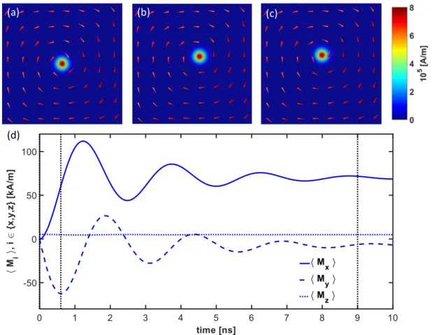
(a) (b) (c)

(d)

Figure 2.7: (a) to (c) show the vortex structure for a 200 nm

200 nm

10 nm permalloy sample at times 0 ns, 0

6 ns, and 9 ns with a constant current density of 5

10

A/m

is applied in

direction. The Gilbert damping parameter is set to

= 0

1. The color coding corresponds to the magnitude of the out of plane component of the magnetization.

The red arrows show the direction of the magnetization as a guide for the eye. (d) The average magnetization components are shown as a function of time. The solid line shows

, the dashed line shows

, and the dotted line

.

When a constant spin polarized current density is applied, the vortex structure

performs a spiral movement until it reaches its new equilibrium position. Fig-

ure 2.7 (b) and (c) show snapshots of the vortex structure for the times 0 . 6 ns and

9 ns. The color coding indicates the magnitude of the out of plane magnetization component. Figure 2.7(d) shows the averaged magnetization components hM

i (solid line), hM

i (dashed line), and hM

i (dotted line) as a function of time. The times corresponding to the snapshots are indicated as vertical black dotted lines.

For a large Gilbert damping constant of 0 . 1 it can be seen easily that the vortex structure has almost reached its new equilibrium position after 10 ns.

To further analyze our numerical results of the gyrotropic motion of temperature driven vortices in small thin film elements we use an analytic solution of the Thiele equation [24], which has been expanded by Thiaville et al. [52] to include a spin polarized current density. By describing the vortex by four triangles, as shown in fig. 2.6, it is possible to establish a direct correspondence between the vortex-core position and the spatially averaged magnetization [51]. In this model it is assumed that the magnetization in each triangle is homogeneous, as indicated by the red arrows in fig. 2.6. Following the derivations of Kr¨uger at al. [51] and neglecting any Oersted field driven magnetization dynamics by assuming a spatially homo- geneous current in x direction, the two dimensional equation of motion for the vortex core position described by the vector ( x ( t ) , y ( t ))

is given by

d dt

x y

!

= − Γ −pω pω − Γ

!

x y

!

+ − (1 +

α

)

pωΓ ω²+Γ²

ξ−α α

!

b

j. (2.6) Here p = ± 1 is the polarization of the vortex core and refers to the magnetization direction of the vortex core, either parallel or antiparallel to the z axis. In the absence of external currents the excited vortex undergoes an exponentially damped spiral rotation until it reaches its equilibrium position. ω is the eigenfrequency of the free vortex motion and Γ is the corresponding damping constant. Assuming a small displacement of the vortex center from equilibrium, the energy of the vortex shifted from its equilibrium position at the dot center can be modeled as a parabolic potential E = ˜ κ ( x

+ y

), with stiffness coefficient ˜ κ [13], which for a circular disk can be approximated by ˜ κ = mu

M

[ F

( g ) − l

/l )

] with g = t/l and the exchange length l

[53]. F

( g ) is given by F

( g ) =

f ( kg ) J

( k ) /kdk with f ( x ) = 1 − (1 − e

) /x and J

( x ) the Bessel function of first order. Within this approximation ω and Γ can be expressed as

ω = − pG

˜ κ

G

+ D

α

and Γ = − D

α ˜ κ

G

+ D

α

. (2.7)

The gyrovector G ~ = G

ˆ e

indicates the axis of precession and is perpendicular to

the film plane. It can be represented with the components of the antisymmetric

gyrotensor and is given by G

= 2 πptM

/ Γ [13]. D

is the non-zero diagonal

element ( D

= D

= D

, D

= 0) of the dissipation tensor and can be estimated

by D

≈ −πM

µ

ln( l/a ) /γ . Assuming that the damping constant of the vortex motion is small compared to its frequency, i.e. Γ

ω

, one can solve this equation [51] and in case of a constant spin polarized electric current density the final core deflection is given by [47]:

∆ x

∆ y

!

= −

Γξ α(Γ²+ω²)

ω (Γ²+ω²)

!

b

j. (2.8)

It is important to note that Γ and ω are itself functions of the Gilbert damping constant α , see equation (eq. (2.7)). However, assuming that the Gilbert damping constant is small, one can use a Taylor series expansion to show that ω , ∆ x

, and ∆ y

only depend on α in second and higher orders. Whereas Γ in leading order is proportional to α . This will become important for the later discussion of the periodically driven vortex motion.

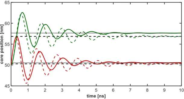
Figure 2.8: Vortex core position (red: x coordinate, green: y coordinate) as a function of time for a 100 nm

100 nm Py sample of thickness 10 nm. The Gilbert damping constant has been set to

= 0

1 and a linear temperature gradient of 1

24

10

mK

nm has been assumed. The solid lines are the core positions determined from the fully micromagnetic simulation, the dashed green and red lines are obtained within the analytic model, and the dotted red and green lines are obtained by fitting to the micromagnetic simulations.

The black dashed and dotted lines correspond to the final stationary core position using an analytic model using the analytic calculated eigenfrequency of the vortex core motion and the eigenfrequency derived from the fitted solution.

Figure 2.8 shows the vortex core position as a function of time for a 100 nm ×

100 nm permalloy sample of thickness 10 nm (red: x ( t ), and green: y ( t )). The

solid line has been determined from the numerical simulations by calculating the

core position. The dashed black lines are the final core positions determined within

the analytic model (see equation (2.8)). The red and green dotted lines have been obtained by a fitting algorithm of the numerical data to the analytical model with ω and Γ as free fitting variables. As starting values for the complex fitting procedure estimates from a Fast Fourier Analysis of the data have been chosen.

The fitted analytic model is in good agreement with the numerical simulations.

To test the scaling behavior full micromagnetic simulations have been performed for lateral dimensions of l ∈ { 100 , 200 , 300 , 400 , 500 } nm and two different linear temperature gradients of 1 . 24 × 10

mK / nm and 1 . 24 × 10

mK / nm corresponding to a spin polarized current density of 5 × 10

A / m

and 5 × 10

A / m

.

(a) (b) (c)

Figure 2.9: (a) Eigenfrequency

=

(2

) of the system for different lateral dimen- sions and thicknesses (10 nm, 20 nm, and 30 nm). (b) Final core position ∆

and (c) final core position ∆

for different lateral dimensions and thicknesses. The lines are calculated within the analytic model (solid lines for a temperature gradient of 1

24

10

mK

nm and dashed lines for a temperature gradient of 1

24

10

mK

nm and the dots are determined from the fully micromagnetic simulations.

Figure 2.9(a) shows the eigenfrequency of the system as a function of the lat-

eral dimension of the square. The lines are calculated within the analytic model

(see equation (2.7)) and the dots show the values determined from the numerical

simulations. Although the analytical model overestimates the frequency, it is in

good agreement with the numerical findings, especially for larger sample sizes, the

agreement between analytical and numerical results becomes very small, which is

especially important when estimating values for larger sized samples which would

be computational time consuming. The different colors indicate different sample

thicknesses. The subfigures fig. 2.9 (b) and (c) show the final vortex core position

as a function of the lateral dimension and sample thickness. In addition two sets

of data are shown corresponding to two different spin polarized current densities

(solid and dotted lines). As expected the magnitude of the final core position

scales with the applied spin polarized current density (see equation (2.8)). Due to

the symmetry of the system, i.e. spin polarized current along the x direction, the

core deflection is much smaller along the x direction than along the y direction,

since this direction is proportional to the non-adiabacity parameter ξ , which is typically relatively small. Another interesting observation is that the analytical model seems to underestimate the final core position. Overall it becomes apparent that the largest movement for the vortex core can be achieved for thin but large samples. This becomes especially important for an experiment using thermal spin transfer torque. So far we have used relatively large temperature gradients, which might be difficult to achieve and maintain in an experimental set up. To overcome this experimental challenge, in the following the vortex motion driven by periodic heat pulses will be considered with the goal to achieve maximal lateral movement and to minimize the involved temperature gradients. For the case that the vortex motion is driven by a series of heat pulses we decouple the equation of motion for the core position and obtain the following second order differential equations:

d

dt

x y

!

+ 2Γ d dt

x y

!

+ ( ω

+ Γ

) x y

!

= −pωb

j +

α

b

− Γ(1 +

) b

j − (1 +

α

) b

!

.

(2.9)

Here the current density is time dependent. Each equation has the form of the differential equation for a damped harmonic oscillator, where the friction is given by 2Γ. In the following we assume that the current varies like j = j

e

, with constant current density j

and driving frequency Ω. The maximum of the dis- placement amplitude is found by solving

d|A

(Ω) |

dt = 0 and d|A

(Ω) |

dt = 0 . (2.10)

This gives a resonance frequency of Ω

= ω

− Γ

. To simplify the following discussion, we assume in addition that the degree of nonadiabaticity is of the same order as the Gilbert damping constant ξ ≈ α . In this case, we can neglect to first order all terms proportional to ( ξ − α )

in the expression of the displacement amplitude and the maximum of the displacement amplitude is given by:

|A

(Ω

) | = |A

(Ω

) | = 1 2 | b

j

Γ | ∝ 1

α . (2.11)

It is obvious that the vortex core motion precesses in the considered case on a

circular path with the given amplitude which is proportional to the spin polarized

current density. Assuming that the Gilbert damping constant α is small, one can

use a Taylor series expansion of Γ and one can show directly that the amplitude

is inversely proportional to the Gilbert damping parameter α . The proportional-

ity relation follows directly from equation (2.7). Therefore materials with a low

Gilbert damping parameter will lead to a larger amplitude of the movement of

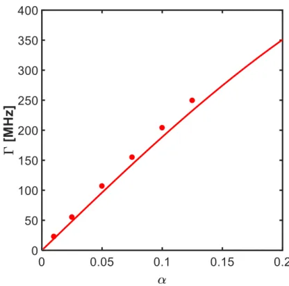
Figure 2.10: Damping constant Γ of the gyrotropic motion of the vortex core as a function of the Gilbert damping constant

. The solid line is determined with the analytic model and the dots are the results from micromagnetic simulations for a 500 nm

×

500 nm

10 nm sample. Γ scales approximately linear for small

.

the vortex core in case one utilizes heat pulses or pulsed currents to generate spin torque driven vortex core motion. The dependence of Γ on the Gilbert damping constant α is shown in fig. 2.10 for a sample size of 500 nm × 500 nm × 10 nm.

The solid line corresponds to the analytical model and the dots are determined

from fully micromagnetic simulations. It becomes obvious that in the case of a

periodically driven vortex motion, the amplitude of the resulting stationary mo-

tion increases in case a material with low Gilbert damping is used, which helps

in the experimental realization to use thermal spin transfer torque to drive and

detect the magnetic vortex core motion. However, from equation (2.11) it becomes

obvious that the maximal amplitude of the driven vortex motion is proportional

to the spin polarized current density which, when created through a temperature

gradient in a permalloy sample, is relatively small and the expected movements of

the vortex core are below 100 nm, which is experimentally very difficult to resolve.

2.3 Extended Thiele Equation for Vortex Core Motion

Based on the good agreement between fully micromagnetic simulations and the analytic solutions from the Thiele equation, an extended form of the Thiele equa- tion is derived in the following section to include, in addition to the conventional spin transfer torque term driven by the inclusion of an electric current density, as discussed in the previous section, terms capturing the thermomagnonic torque, also often referred to as magnon spin transfer torque, as well as thermal fluctu- ations. The discussion of pure thermomagnonic torque has recently become the focus of studies in insulating ferrimagnets, such as yttrium iron garnet (YIG) [54], and magnetic insulators, such as Cu

OSeO

[55], BaFe

Sc

Mg

. 05O

9 [56], and Y

Fe

O

[57]. Here special emphasis has been on the study of domain wall driven motion [58, 59] and the manipulation of skyrmions [59, 60]. But also in con- ducting materials, as in the considered permalloy sample, pure thermomagnonic spin torques can couple the magnetic moments to the temperature gradient even in the absence of electric charge flows [45, 61]. The generalized Thiele equation, which describes the vortex core motion as discussed in the previous section, has the following form:

F ~ + G ~ × V ~ + α D ~ ˆ V = 0 . (2.12) Here V ~ = d ~ R/dt is the velocity of the vortex core and R ~ = ( x ( t ) , y ( t )) is the vortex core position. As introduced in the previous section G ~ is the gyrovector and ˆ D the dissipation tensor. The force vector F ~ includes now the force due to the stray field ( F ~

), spin transfer torques via electric currents F ~

, pure thermomagnonic torques ( F ~

), and thermal fluctuations ( F ~

). Using the superposition principle the force can therefore be written as

F ~ = F ~

+ F ~

+ F ~

+ F ~

. (2.13) The force due to the stray field can be again derived by assuming a parabolic potential with stiffness constant ˜ κ as discussed in the previous section:

F ~

= −mω

x ˆ e

− mω

y e ˆ

with ˜ κ = 1

2 mω

. (2.14) The force due to electric charge currents has been discussed in detail in the previous section and is given by:

F ~

= b

G ~ × ~j + ξb

D~j, ˆ (2.15)

where b

describes again the coupling between the magnetization and the electric

charge carriers. Since the parameter ξ , which describes the degree of nonadia-

baticity, is often very small, the force is often approximated by F ~

≈ b

G ~ × ~j .

To include a pure thermomagnonic torque, we follow the approach chosen by Tatara [59]. In the case of transport phenomena attributed to charge carriers, Luttinger introduced a fictitious scalar field, also called gravitational potential, which couples to the local energy density by an interaction Hamiltonian [62]. Sev- eral approaches have been attempted to apply a similar formalism to pure thermal case. However, those approaches often led to wrong thermal coefficients [63, 64] or nonphysical divergences arose from an unmodified approach [65]. Those difficulties can be prevented by replacing the scalar potential formalism by a vector poten- tial formalism [66, 67]. The vector potential form of the interaction Hamiltonian describing the thermal effect is given by

H

≡ −

Z

~j

( ~ r, t ) · A ~

( ~ r, t ) d

r, (2.16) where A ~

( ~ r, t ) = ∇T /T ~ is the thermal vector potential and ~j

( ~ r, t ) the energy current density. Following the approach by Tatara [59], one can now calculate the thermally driven dynamics of a spin structure as a linear response to the interaction Hamiltonian (2.16) and the force in the extended Thiele equation takes the following form

F ~

= 2 J a

~

G ~ × ~j

. (2.17)

In the equation above one has already made the assumption that the magnon current density is an effective 2 d current density within a thin film plane, i.e.

~j

= ~j

t . As defined in the previous section, t is the thickness of the permal- loy sample, J the exchange constant, and a the lattice parameter. Applying a semiclassical approach with the relaxation time approximation [68] the magnon current can be expressed as

|~j

| = a

(2 π )

Z

k

(ˆ a )

(ˆ a )

d

k (2.18) where (ˆ a )

and (ˆ a )

are the magnon creation and annihilation operator. Neglecting higher order processes, such as magnon-magnon interactions, one can show that the relaxation time is determined only by the Gilbert damping parameter α and the magnon current, here assumed to be parallel to the x axis, is given by [23]

j

= π

26 a

( k

~ v

)

T α

dT

dx , (2.19)

where v

is the effective velocity of the magnon, and k

the Boltzmann constant.

The effective magnon velocity can be estimated via v

=

, which gives

for permalloy a value of approximately 1010 m / s, which is two orders of magni-

tude larger compared to the antiferromagnet Cr

O

[69].

To introduce a force describing thermal fluctuation, one has to introduce stochastic fields whose time correlations satisfy the fluctuations-dissipation theorem [70, 71].

This approach is similar to fully micromagnetic simulation including a random stochastic field ν ~ H

with stochastic parameter ν to mimic temperature fluctu- ations. However, since we are only interested in the overall magnitude of the resulting motion, we chose a simplified approach by introducing a direct force as done by Tatara [59]. Here the direct force arises from the annihilation of vortices contributing to the entropy production. The direct thermal force can be expressed as

F ~

= γ

T

∇T. ~ (2.20)

Since the annihilation of vortices requires a finite excitation energy, the parameter γ

vanishes fast as the temperature approaches zero. Therefore the force vanishes at T = 0. The parameter γ

can be estimated using the fluctuation dissipation theorem [72], where the stochastic parameter ν

is given by the ratio of the thermal energy to the magnetic energy:

ν

≈ 2

k

T

µ

M

V , (2.21)

where V is the sample volume. One can now use the nominator to approximate the prefactor of the force caused by thermal fluctuations entering the Thiele equation:

γ

T ≈ 2

k

T

T ≈ 2 k

α

1 + α

. (2.22)

Since the velocity of the vortex core is in the film plane, and therefore perpendic- ular to the gyrovector, one can rewrite the generalized Thiele equation (2.12) in the following form:

G ~ × F ~ − G

V ~ + αD

G ~ × V ~ = 0 . (2.23) Using the expression for G ~ × V ~ from (eq. (2.23)) and inserting this expression into the original equation (2.12), one can derive the following equation for the velocity of the vortex core:

( G

+ α

D

) V ~ = G ~ × F ~ − αD

F . ~ (2.24)

To discuss the different contributions from a charge current and a pure magnon

current, a homogeneous charge current parallel to the x axis and a linear tem-

perature gradient along the x axis is taken into consideration. In the absence of

a charge current, a pure magnon current, and any thermal fluctuation, just in-

cluding the force F

for the stray field, the energy landscape of the vortex has its

minimum in the center of the sample. An excited vortex, i.e. a vortex with the

core not in the center position, performs an exponentially damped spiral rotation around its equilibrium position with the angular eigenfrequency

ω = − pG

mω

G

+ α

D

, with ˜ κ = 1

2 mω

, (2.25)

and the damping constant

Γ = − αD

ω

G

+ α

D

. (2.26)

From the two equations above, equations (2.25) and (2.26), one obtains the fol- lowing relation

αD

= p Γ G

ω . (2.27)

Using equation (2.27), and the following relations pω Γ

ω

+ Γ

= αD

G

G

+ α

D

, (2.28) ω

ω

+ Γ

= G

G

+ α

D

, and (2.29) Γ

ω

+ Γ

= α

D

G

+ α

D

, (2.30) one obtains the following equations of motion for the x and y coordinates of the vortex core:

dx

dt = − pωy − Γ x − (1 + Γ

ω

+ Γ

ξ − α α ) b

j

− ω

ω

+ Γ

2 J a

~ j

− Γ

ω

+ Γ

γ

T

∂T

∂x , dy

dt = + pωx − Γ y + pω Γ ω

+ Γ

ξ − α α b

j

− pω Γ ω

+ Γ

2 J a

~

j

+ ω

ω

+ Γ

1 G

γ

T

∂T

∂x . (2.31)

Here the first two terms in each equation are responsible for the damped spiral

rotation, the second terms are proportional to the involved charge current density

and describes the motion due to the spin transfer torque connected to charge car-

riers. The third terms are proportional to the pure magnon current and describe

therefore the pure magnonic motion of the vortex core. The last terms in each

equation describe the average motion of the vortex core due to random thermal

fluctuations. It should be mentioned here that a fully micromagnetic code, which

includes thermal fluctuations along a temperature gradient, would be able to fully

describe the motion, hereby replacing the last two terms in the equations of mo-

tion. While fully micromagnetic simulations including a stochastic field can be

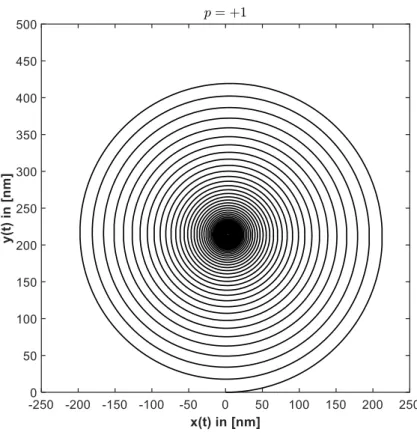
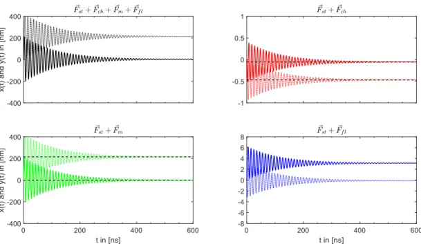
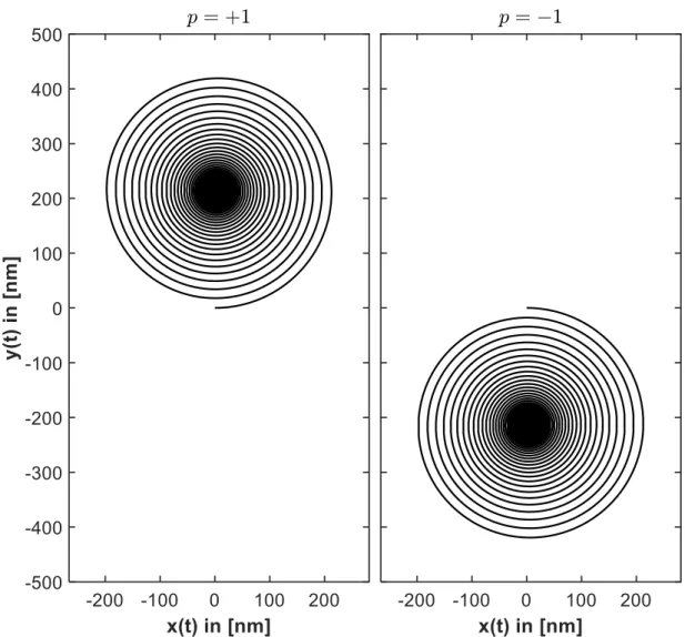
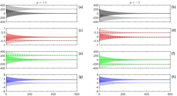
done assuming a constant temperature within the sample (see for example [70]) we are not aware of the attempt to do so including a temperature gradient. The inclusion of a temperature gradient would require an extremely small time step in the micromagnetic simulations to cover the pure magnonic motion correctly. To evaluate the vortex core motion and compare the results to experimental data, we have solved the equations of motion (2.31) numerically. The main advantage of this method is that one can analyse the different contributions to the final core po- sition separately. The resulting core motion can be again described by a damped spiral motion, starting at the center of the sample, i.e. at R ~ ( t = 0) = (0 , 0) and ending at the new equilibrium position R ~ ( t → ∞ ) = (∆ x, ∆ x ), as shown in fig. 2.11.

Figure 6: Sample geometry for the extended Thiele equation. At the beginning the vortex core is at the center of the sample, i.e.! = 0,0 and shown as grey dot. Due to the additional forces, the vortex core undergoes a damped spiral rotation into its new equilibrium position, i.e.! = (Δ', Δ()and shown as red dot.

Figure 2.11: Sample geometry for the extended Thiele equation. At the beginning the vortex core is at the center of the sample, i.e.

= (0

0) and shown as grey dot. Due to the additional forces, the vortex core undergoes a damped spiral rotation into its new equilibrium position, i.e.

= (∆

∆

) and shown as red dot.

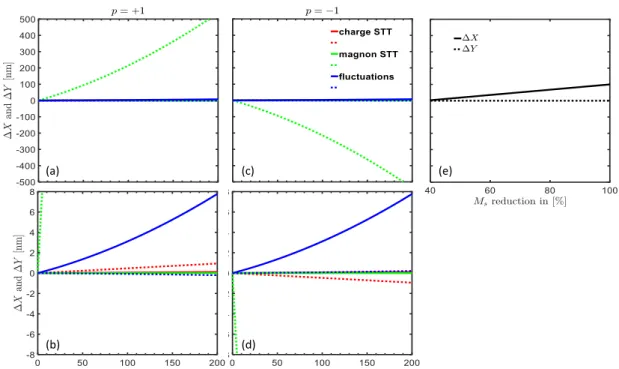
Similar to the case discussed in the previous section, where only a spin polar- ized charge current has been considered, it is possible to calculate the final core position analytically. Neglecting the forces due to spin polarized charge currents and random thermal fluctuation, the equations of motion (2.31) are given by

dx

dt = − pωy − Γ x − v

, dy

dt = + pωy − Γ x − v

. (2.32)

Here the components of the magnon velocity vector are defined as v

= ω

ω

+ Γ

2 J a

~

j

, v

= pω Γ

ω

+ Γ

2 J a

~

j

. (2.33)

In order to calculate the final core deflection due to the pure magnon transfer torque, the solution for the vortex core needs to be stationary, i.e.

=

= 0.

Under this condition the final core deflection is given by:

∆ x

∆ y

!

= 1

Γ

− ω

− Γ v

+ pωv

pωv

− Γ v

!

= 0

−

~

j

!

. (2.34)

This result can be directly compared with the obtained numerical results by solving the generalized equations of motion (2.23).

In the following, numerical solution of the extended Thiele equation (2.12) will be discussed including the forces associated with the stray field, the spin transfer torque via electric and pure magnon currents, and thermal fluctuations. Besides the previously discussed parameters, a saturation magnetization of 8 × 10

[A/m], a Gilbert damping constant of 0 . 006 [73], and a non-adiabaticity parameter of 0 . 05 [47] are used. According to the experiment the lateral sample dimension is chosen to be 2 µ m and the sample thickness is 20 nm. Starting with the vortex core in the center of the sample, the resulting vortex core motion can be described again by a damped spiral rotation approaching the new equilibrium position, which in this case differs from the central position due to the involved forces. Such a motion is shown in fig. 2.12 for a vortex polarity of p = 1 and a chirality of c = 1. At t = 0 the vortex core is in the center of the sample, i.e. R ~ = (0 , 0).

To analyze the different contributions to the overall vortex core motion, the x -

and y -amplitudes are shown separately in fig. 2.13(a). The x -component of the

vortex core is shown as a solid line, and the y -component of the vortex core is

shown as a dotted line. For the case where only the charge spin transfer torque or

the thermomagnonic torque are considered, the analytic solutions (see equations

(2.8) and (2.34)) are shown as black dashed lines. By analyzing the contributions

to the final core position, one finds that the motion induced by spin transfer torque

due to spin polarized charge currents is as expected zero in the direction of the

temperature gradient (parallel to the x axis). However, it has a non-vanishing

component in the direction perpendicular to the temperature gradient (parallel

to the y axis). As already discussed in the previous section using this approach

as well as fully micromagnetic approach, the final core deflection ∆ y is relatively

small (see fig. 2.13 (b)). With a temperature gradient of 100 [mK/nm] which cor-

responds to a charge current density of 4 × 10

A/m

this contribution is below

1 nm. This small movement is mainly caused by the relatively small spin-Seebeck coefficient for permalloy and leads to a relatively bad efficiency to create charge currents using a temperature gradient. This movement is certainly below the res- olution feasible in an experimental setup. However, the movement induced by pure magnon currents is for the given situation in the order of a few hundred nm.

As can be seen in fig. 2.13(c) the final core deflection perpendicular to the tem-

perature gradient is zero, as also expected from the analytic solution for the final

core position. The final core position perpendicular to the temperature gradient

is at 215 nm and therefore possible to detect experimentally. Using the involved

magnon velocities in equation (2.33) and equations (2.28) and (2.29), one can eas-

ily show that the magnon velocity in the y direction, i.e. perpendicular to the

temperature gradient, is proportional to the Gilbert damping parameter α and

therefore much smaller than the magnon velocity in the x direction, i.e. parallel

to the temperature gradient. For the considered case the magnon velocity in the y

direction is about 70 times larger than the magnon velocity in x direction. A sim-

ilar behavior has been derived theoretically for the magnon velocity for thermally

driven skyrmions [23]. In fig. 2.13(d) the average contribution accounting for ther-

mal fluctuations are shown. Due to the random nature of those fluctuations, a

final core deflection parallel and perpendicular to the temperature gradient is ex-

pected. For the assumed temperature gradients, those movements are in the order

of 3 nm, which has been also shown using a stochastic Landau Lifshitz equation

by Machado et al. [70]. Therefore only the movement caused by pure magnon

currents is accessible in an experimental setup.