Wall Motion in Magnetic Nanostructures
Dissertation
zur Erlangung des Doktorgrades der Naturwissenschaften (Dr. rer. nat.)
der Fakultät für Physik der Universität Regensburg
vorgelegt von
Tobias Weindler
aus Teublitz im Jahre 2017
Prüfungsausschuss: Vorsitzender:
1. Gutachter:
2. Gutachter:
weiterer Prüfer:
Prof. Dr. Gunnar Bali Prof. Dr. Christian Back Prof. Dr. Dieter Weiss PD Dr. Jonathan Eroms
1 Introduction 1
2 Theoretical Background 5
2.1 Landau-Lifshitz-Gilbert Equation . . . . 5
2.2 Thiele Equation . . . . 7
2.2.1 Basic Idea . . . . 8
2.2.2 Equivalent Field Equation . . . 10
2.2.3 Effective Force Density and Force Equation . . . 12
2.2.3.1 Steady-State Motion . . . 13
2.2.3.2 Magnetization Equivalent Term . . . 22
2.2.3.3 Force Term . . . 22
2.2.3.4 Damping Equivalent Term . . . 23
2.2.3.5 Gyroscopic Term . . . 26
2.2.4 Thiele Equation . . . 30
2.3 Dynamics of Vortex Domain Walls . . . 31
2.3.1 Vortex Domain Walls . . . 31
2.3.2 Vortex Domain Wall Motion in the Frame of the Collective Coordinate Approach . . . 36
2.3.2.1 Generalization of Thiele’s Analysis: Generalized Coordinates, Forces and Velocities . . . 39
2.3.2.2 Special Physical Quantities used in the Collective Coordinate Approach . . . 42
2.3.2.3 Concept of Modes . . . 49
2.3.2.4 Energies . . . 54
2.3.2.5 Force Term . . . 55
2.3.2.6 Gyrovector . . . 56
2.3.2.7 Damping Tensor for a Vortex in a Disc . . . 58
2.3.2.8 Damping Tensor for a Vortex Domain Wall . . . 61
2.3.2.9 Equation of Motion in the One-Dimensional Case 66 2.3.2.10 Equation of Motion in the Two-Dimensional Case 67 2.3.3 Solution for the Equation of Motion of a Vortex Domain Wall in the Framework of the Collective Coordinate Ap- proach . . . 70
2.3.3.1 Solution for the Equation of Motion in the One-
Dimensional Case . . . 70
2.3.3.2 Solution for the Equation of Motion in the Two- Dimensional Case . . . 71
2.4 Ferromagnetic Resonance . . . 75
2.4.1 Considerations Regarding the Coordinate System: How to Solve the Landau-Lifshitz-Gilbert Equation in the Case of Ferromagnetic Resonance . . . 76
2.4.2 Solutions for Ferromagnetic Resonance in the Full-Film and Stripe Geometry . . . 85
2.5 Magneto-Optical Kerr Effect . . . 88
2.5.1 Quantum Mechanical Origin of the Magneto-Optical Kerr Effect . . . 89
2.5.2 Magneto-Optical Kerr Effect in the Frame of Classical Optics 91 3 Experimental Techniques and Data Evaluation 93 3.1 Sample Design . . . 93
3.2 Superconducting Quantum Interference Device . . . 98
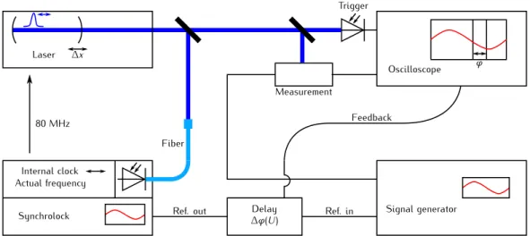
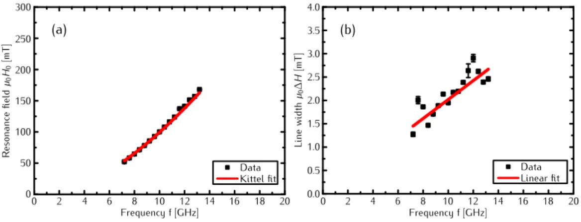
3.3 Time-Resolved Kerr Microscopy . . . 98
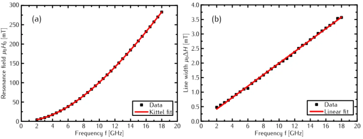
3.4 Full-Film Ferromagnetic Resonance . . . 104
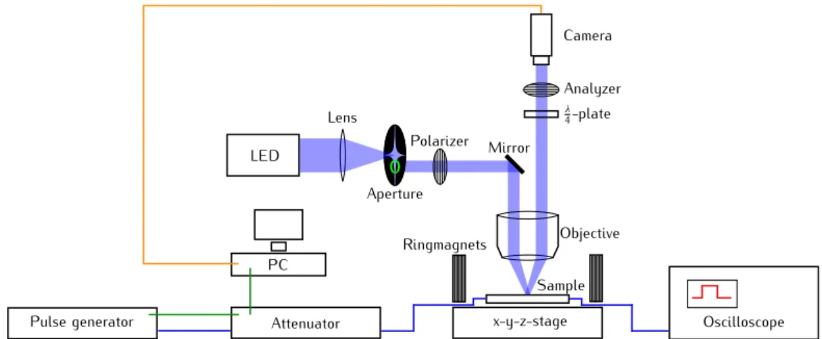
3.5 Wide-Field Kerr Microscopy . . . 105
3.6 Evaluation of Measurement Data . . . 107
3.7 Evaluation of Simulation Data . . . 109
4 Experimental Results and Simulations 111 4.1 Sample Characterization . . . 111
4.1.1 Superconducting Quantum Interference Device Measure- ments: Determining the Saturation Magnetization . . . 111
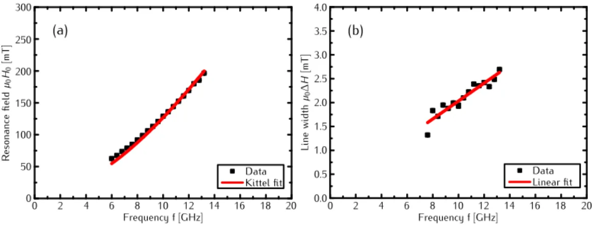
4.1.2 Full-Film Ferromagnetic Resonance Measurements: Deter- mining the Magnetic Damping Parameter . . . 112
4.1.3 Ferromagnetic Resonance Measurements with Time-Resolved Kerr Microscopy: Determining the Magnetic Damping Pa- rameter . . . 113
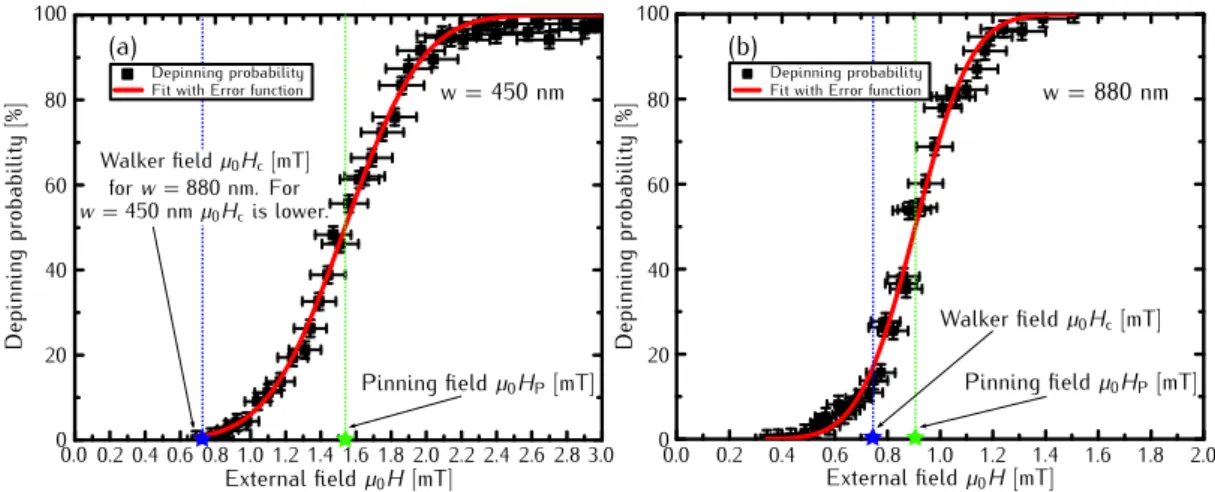
4.1.4 Depinning Probabilities in the Relevant Field Range and the Depinning Field . . . 116
4.1.5 Low-Field Mobility and the Walker Field . . . 117
4.2 Chirality-Dependent Vortex Domain Wall Dynamics and the Dou- ble Reversal Process . . . 119
4.2.1 Introduction . . . 119
4.2.2 Chirality Dependent Vortex Domain Wall Dynamics: An Analytical Approach . . . 120
4.2.3 Chirality Dependent Vortex Domain Wall Dynamics: Mi- cromagnetic Simulations . . . 123
4.2.4 Chirality Dependent Vortex Domain Wall Dynamics: Ex- perimental Data . . . 125
4.2.5 Double Reversal Process: A Descriptive Approach . . . 127
4.2.6 Double Reversal Process: Basic Considerations for Trace, Energy and Potential . . . 130
4.2.7 Double Reversal Process: A Detailed Discussion for Trace,
Energy and Potential . . . 133
4.2.8 Double Reversal Process: Influence of the Spin Wave Pack- age . . . 139
4.2.9 Double Reversal Process: Considerations in the Frame of Gyrofieldhgyro and Zeeman Energy Caused by it . . . 144
4.2.10 Double Reversal Process: The Effective Potential for VC and Dip Region . . . 148
4.2.11 Double Reversal Process: Influence of the Half Antivortices 149 4.2.12 Conclusion . . . 152
Summary 155 Appendix 159 A1 Short Introduction into the Tensor Calculation with the Outer Product . . . 159
A2 Short Introduction Into the Generalized Kronecker Delta and the -Tensor . . . 163
A3 Unit Vectors and the Nabla Operator in Spherical and Cylindrical Coordinate System . . . 166
A4 Characterization of the Field Pulses . . . 169
A5 Calculation of U(X) and Average Velocity ¯V During the Double Reversal Processes . . . 172
A6 Trace and ETot,DW for Eight Double Reversal Processes . . . 173
A7 Dividing the Domain Wall in Subsystems . . . 175
A8 Evaluation of the Spin Wave Package . . . 175
A9 Determination of the Domain Wall Velocity via Gyrofield hgyro . . 177
A10 Pictures for Gyrofield and Egyro,z for One Complete Double Re- versal Process . . . 178
Acknowledgements 181
Abbreviations 185
Publications 187
Bibliography 189
Introduction
This thesis deals with the research area of domain walls (DW). In particu- lar, the dynamics of field-driven vortex domain walls (VDW) in nano-stripes is investigated experimentally as well as by means of analytical calculations and micromagnetic simulations. But why should you do research in this small sub- area of magnetism? It is important and interesting in both, the point of view of technological applications and the fundamental research of solid state physics.
Concerning technological applications, novel storage and sensor devices relying on DWs and VDWs have been proposed respectively [1–3]. Compared to cur- rently existing technologies, an enhanced performance is expected. For instance, the racetrack memory proposed in 2008 by S. S. P. Parkin [1] operates like a shift register [2] and should combine as non-volatile memory device the high performance and reliability of solid-state memories, and at the same time it has the low costs of disc-drive storages. In a racetrack memory the information is stored in a magnetic thin film stripe geometry where the in-plane magnetized domains represent the "0" and "1" bits. Reading the information can be realized by magnetic tunnel junction magnetoresisitive sensing devices [4], while the writ- ing of bits is possible through different methods, for example, spin-momentum transfer torque (SST) [5, 6]. The shifting of the domains, which encode the digital information, is done also by spin-momentum transfer torque mediated by a spin-polarized electric current, which naturally arises when injecting an electric current into a magnetic material. How reliable and fast the domains can be shifted depends strongly on the dynamics of the DWs between domains with opposing magnetization direction. Aiming to build such storage media, a deep understanding of DW dynamics is a necessary prerequisite. Further pro- posed technological applications are magnetic sensors based on VCs and VDWs.
Currently used micromagnetic sensors play a key role in a large variety of in- dustry branches, for example, the automotive industry, where they are used for speed and position detection [3]. These sensors consist of a patterned magnetic element and a magnetoresistive sensor which utilizes effects, such as the giant magnetoresistance (GMR) [7–9], anisotropic magnetoresistance (AMR) [10] and tunnel magnetoresistance (TMR) [9, 11, 12]. However, actual sensors suffer from
a non-linear hysteresis curve and a high magnetic noise level. Micrometer-large ferromagnetic discs containing a magnetic vortex state are regarded as possible solution to avoid the latter mentioned limitation [3]. These sensors are proposed to operate with a higher linear regime and a magnetic noise level, which is an order of magnitude lower compared to actual used sensors. Therefore, a deep understanding of the complicated VC dynamics is necessary in order to build such a device. As it will become clear by the work done in this thesis, VDW are, besides the investigation of VCs in a disc [13–16], a possible way to tackle the investigation of VC dynamics. Of course, the investigation of DWs is important for basic research as well because on the one hand, side DW dynamics itself pro- vides a huge variety of different aspects that can be discovered and which leads to a deeper understanding of DW and magnetization dynamics itself; on the other hand, it is a practical way to investigate certain basic material properties.
Concerning the DW dynamics itself, examples are domain wall motion (DWM) at low and very high fields [17, 18] and by STT [19], DW depinning [20] and VC switching processes [21]. From the point of view of material properties, DW dynamics, especially the DWM of VDW, offers a convenient way to investigate magnetic damping mechanisms [22]. In the Landau-Lifshitz-Gilbert equation (LLG equation) [23–25] magnetic damping, and so the energy dissipation in the physical system, is parametrized by a scalar factor α. This implies that the energy dissipation is independent on the magnetic texture itself. However, an additional magnetic texture which depends on damping mechanism called non- local damping is proposed [26–28]. This additional damping enters respectively the LLG equation by an extra term proportional to a material parameter η, the spatial magnetic gradient and its time derivative. In order to catch effects of non-local damping, a fast moving magnetic texture is required, ideally accom- panied with a strong magnetic gradient. Field driven VDWs in stripes provide such a toy model because they exhibit a natural given strong magnetic gradient due to the VC in the bulk and the half anti-vortices (HAVs) located at the edges.
These three objects form together a VDW and strongly influence the dynamics of the DW. Because of their strong magnetic gradient, they are sensitive to non- local damping, and a possible effect should be, if large enough, measurable by DWM in the linear regime. A better overall understanding of the basic science of DWs has a retroactive effect on the earlier mentioned technological applica- tions allowing to tailor the materials and magnetic systems to the respective requirements.
This thesis focuses on a special aspect of VDW dynamics arising in relatively wide stripes at fields above the Walker breakdown (WB) [29]. Differences for the breakdown mechanism of VDW with different chirality χ are evidenced by experimental data, analytical calculations and micromagnetic simulations. A new behaviour of VDWs with chirality χ = +1 is discovered above the WB being causal for the mentioned different breakdown mechanism.
The thesis is organized as follows: In Ch. 2 the theoretical background for the investigation of DWM is set. Starting in Sec. 2.1 with the basic equation of magnetization dynamics (LLG eq.) and its basic properties, the considerations proceed to the reformulation of this equation into an equivalent force equation
cussed in the context of VDW motion in Sec. 2.3. The chapter ends with Sec. 2.4 and Sec. 2.5 where the theoretical background for the measurement techniques is provided. In Ch. 3 the experimental techniques and the way the acquired data were evaluated is presented. In Sec. 3.1 the sample design is explained, while Sec. 3.2-3.5 presents the measurement techniques superconducting quan- tum interference device (SQUID), time-resolved Kerr microscopy (TR-MOKE), full-film ferromagnetic resonance (full-film FMR) and wide-field Kerr microscopy (wide-field MOKE) which were utilized in this work. Subsequently the data eval- uation of the obtained measurement and simulation data (Sec. 3.6 and Sec. 3.7) is described. In Ch. 4 the experimental results and the data from micromagnetic simulations are shown. Sec. 4.1 gives an overview of the results obtained from the sample characterization, while in Sec. 4.2 the chirality-dependent VDW dy- namics is evidenced and discussed from different points of view. This thesis is closed by Ch. 4.2.12 and ends with the appendix .
Theoretical Background
In this chapter the theoretical foundations for understanding and describing the DWM are laid. Beginning with the description of the basic equation of mag- netization dynamics (LLG eq., Sec. 2.1), a conversion into a more suitable force equation with respect to DWM follows (Thiele eq., Sec. 2.2). Sec. 2.3 contains the detailed discussion of the dynamics of VDWs in the frame of the Thiele equa- tion. The chapter is closed by the presentation of the theoretical background for the measurement methods of FMR and Kerr microscopy in Sec. 2.4 and Sec. 2.5, respectively. As starting point of the theoretical considerations, the LLG eq.
and its basic properties are introduced in the subsequent section.
In order to provide the theoretical background for magnetization dynamics and domain wall motion in Ch. 2, many intermediate steps for calculations and derivations are given; this concerns especially Sec. 2.2. However, detailed cal- culations are hard to find in available literature except some PhD theses like Krüger’s Current-Driven Magnetization Dynamics [30]; Nevertheless, they are helpful to get into the topic of domain wall motion from the theoretical point of view, and so the calculation steps that were carried out by myself will be marked with the footnote "1".
2.1 Landau-Lifshitz-Gilbert Equation
Aiming to describe magnetization dynamics from a theoretical point of view, an equation that describes the time evolution of the magnetization vectorM~ under the influence of different interactions is required. Besides different approaches to differential equations [31], the most common one is the Landau-Lifschitz equation (LL equation), which was formulated in 1935 [23]. It was modified later on by Gilbert in 1955 in order to adjust it to a Lagrangian formalism and to convert it to friction like damping [24, 25]. The Landau-Lifshitz-Gilbert equation (LLG equation) reads
dM~
dt =−γ0M~ ×H~eff+ α Ms
M~ × dM~
dt (2.1)
Figure 2.1. The sketch depicts the magnetization dynamics governed by the LLG equation. Having a magnetization M~ deflected by an angle ϑ from the effective field H~eff, two different torques are present which sum up to the total changing rate ddtM~ .
−γ0M~ ×H~eff is the precessional torque causing a precession ofM~ around the effective fieldH~eff, while Mα
s
M~ ×ddtM~ (the damping term) is forcing the magnetization to align parallel to the effective field.
and states that the time change rate ddtM~ of the magnetization M~ is governed by two terms, the precessional (first one) and the damping term (second one).
The LLG eq. as well as the LL eq. can be derived from a phenomenological [23, 32] or quantum mechanics point of view [33]. The factor γ0 is given by
−µ0γ, where γ is the gyromagnetic ratio and µ0 is the magnetic permeability of the vacuum. The effective field H~eff contained in the precessional term is determined by the variational derivative of the energy density E of the physical system with respect to M~ and given by [32]:
H~eff =− 1 µ0
δE
δ ~M (2.2)
In the damping term,αis the Gilbert damping parameter, which is a material- dependent key number that quantifies the dissipation rate of energy in the sys- tem. Concerning the two terms describing the time evolution ofM~, they can be understood in the following way: Neglecting the damping term, it is found that the time change rate of the magnetization is governed solely by the precessional term. This precessional term is very similar to the equation of the motion of a gyroscope. Having a torque acting on a spinning gyroscope, it starts to precess around its initial equilibrium position. In the same way it is the case for the magnetization; when an effective field, which can constitute out of an external field and different physical interactions, is acting onM~, the magnetization starts to precess around its equilibrium position.
This precessional motion would continue forever if the damping and energy dissipation were absent, respectively. However, from experimental results it is a well known fact that the magnetization aligns very fast along the effective field. To take this fact into account, a damping term has to be included. Such a damping term has to leave the length of the magnetization vector unchanged
because the conservation of saturation magnetizationMsis assumed. Due to this reason, it has to be perpendicular to the vectorM~, and the only way to formulate the desired term is as it is done in Eq. (2.1). For the sake of completeness it should be noted, that the termM~ ×ddtM~ can be written as M~ ×M~ ×H~eff as well - an equivalent notation used for example in the original work by Landau and Lifschitz [23]. Conservation of saturation magnetization with respect to time leads to interesting consequences for the terms contained in the LLG equation.
This will be helpful later on when an equation for the description of DWM based on the LLG equation (see Sec. 2.2) is derived. Preservation of Ms can be demonstrated by multiplying all terms in the LLG eq. by M~ yielding1 [32]:
M~ · dM~ dt = 1
2 d dt
M~2
=−γ0M~ ·M~ ×H~eff
| {z }
=0
+ α Ms
M~ ·
M~ ×dM~ dt
| {z }
=0
= 0 (2.3)
As result1
d
dt|Ms|= 0 (2.4)
the conservation of the saturation magnetization is obtained. Additionally, it can be concluded, due to the fact that the two terms on the right side are equal zero, that they are perpendicular to M~ [32].
M~ ⊥M~ ×H~eff ⊥M~ ×dM~
dt (2.5)
Furthermore, Eq. (2.3) states that the dot product of the magnetization with its own time change rate is zero. Because of this fact, M~ and ddtM~ are perpendicular to each other1.
M~ ⊥ dM~
dt (2.6)
However, since all vectors are perpendicular with respect to the magnetiza- tion vector, care should be taken to M~; but only M~, M~ ×H~eff and M~ × ddtM~ are forming an orthogonal basis and are orthogonal regarding each other respec- tively [32]. Based on this prerequisites, the theoretical considerations evolve to the derivation of an equation which is more suitable for the description of DWM.
2.2 Thiele Equation
In this section the basic equation for the investigation of DWM, the Thiele equa- tion, is derived. As a starting point, the basic idea behind the Thiele equation explained in Sec 2.2.1 and the conversion of the LLG eq. into an equivalent field eq. (Sec. 2.2.2) is demonstrated. These results lead to an effective force den-
1 This calculation has been carried out by myself.
sity and force equation (Sec. 2.2.3), respectively, and they result in the Thiele equation discussed in Sec. 2.2.4.
2.2.1 Basic Idea
The basic idea behind the Thiele equation [34] is to consider the domain wall as a rigid magnetic particle which is not deforming while moving along the stripe with a constant velocity (steady-state motion). Having a rigid particle, the total force acting on the domain wall itself can be considered, so that it is possible to write an equation of motion for the case of steady-state motion as1 [34, 35]:
X
x
F~x= 0 (2.7)
Here, x stands for the different forces arising from the LLG equation. So it should be thought about the force acting on a magnetic texture under the influence of an external magnetic field. Starting with the force that acts on a magnetic dipole and extending it to the magnetization, the potential energy EPot,ix of a magnetic dipole (with magnetic moment ~µis) in an external field H~x is given by1 [36, 37]:
EPotx ,i =−µ0~µis·H~x (2.8) Summing up over all magnetic moments in a volumeV, whereby the assump- tion is taken that one magnetic moment covers a volume Vi, the corresponding energy density is obtained1 [37, 38]
Ex = PNi EPot,ix
PN
i Vi =−µ0
PN i ~µis
PN
i Vi ·H~x=−µ0M~ ·H~x (2.9) which is caused by the influence of a field H~x. Here, the definition was used with the result that the magnetization is given by the total amount of magnetic moments per volume [38]. The total energy density E is obtained by summing over all fields H~x 1:
E =X
x
Ex =−µ0X
x
M~ ·H~x =−µ0M~ ·X
x
H~x=−µ0M~ ·H~eff (2.10) Here, the sum over the different field contributions H~x is denoted as the effective fieldH~eff [32] (see Sec. 2.1). By integrating over the full volume V, the energy E
E =X
x
Ex =X
x
Z
V
ExdV
=X
x
−µ0
Z
V
M~ ·H~xdV =−µ0
Z
V
M~ ·X
x
H~xdV
(2.11)
is found1, which is equal to the Zeeman energy [36–38]. The force density is given by the derivation of the energy density with respect to the spatial compo- nents. Assuming the field H~x as spatially constant, it yields1 [39, 40]:
Ex =−µ0MxHxx+MyHyx+MzHzx (2.12) and the force density vector f~x originating from one certain field H~x reads1 [34, 38, 41]
f~x =−∇E~ x =µ0
∂Mx
∂x Hxx ∂M∂xyHyx ∂M∂xzHzx
∂Mx
∂y Hxx ∂M∂yyHyx ∂M∂yzHzx
∂Mx
∂z Hxx ∂M∂zyHyx ∂M∂zzHzx
=µ0
∂Mx
∂x
∂My
∂x
∂Mz
∂x
∂Mx
∂y
∂My
∂y
∂Mz
∂y
∂Mx
∂z
∂My
∂z
∂Mz
∂z
| {z }
=JT~
M
Hxx Hyx Hzx
=µ0JMT~H~x =µ0
∂ ~M
∂ ~R
T
H~x
(2.13)
whereby the matrix which contains the spatial derivatives is identified as the transposed Jacobian matrix JT~
M [41, 42] of the magnetization M~. Additionally, it is possible to write the transposed Jacobian matrix JMT~ in symbolic notation
∂ ~M
∂ ~R
T
, which will be utilized in the following considerations. Then, the total forceF~ is found by summing over all fieldsx 1.
F~ =−∇E~ =−X
x
∇E~ x=−X
x
Z
V
∇E~ x dV
=X
x
µ0
Z
V
∂ ~M
∂ ~R
T
·H~xdV =µ0
Z
V
∂ ~M
∂ ~R
T
·X
x
H~xdV
(2.14)
Neglecting the integration over the volume yields the force densities1 [34].
f~x =µ0
∂ ~M
∂ ~R
T
·H~x (2.15)
f~=X
x
f~x =µ0X
x
∂ ~M
∂ ~R
T
·H~x =µ0
∂ ~M
∂ ~R
T
·X
x
H~x (2.16)
Therefore, the question arises what the fields are contributing toH~eff and how they are including the dynamics given by the basic equation of magnetization dynamics (LLG eq.). Finding the answer to this question is the task of the next section.
2.2.2 Equivalent Field Equation
The latter question gets a first answer by calculating the force in an alternative manner. Another way is to start from the expression of the energy, applying the nabla operator and using the chain rule in combination with the variation derivative of the energy density concerning the magnetization vector M~ 1 [32, 38, 43].
F~ =−∇E~ =−
Z
V
∇E~ dV =−
Z
V
δE δ ~M
∂ ~M
∂ ~R dV
=µ0
Z
V
H~effT ∂ ~M
∂ ~R dV =µ0
Z
V
∂ ~M
∂ ~R
T
·H~effdV
(2.17)
Since the total energy density of the system is under consideration, the vari- ational term gives −µ0H~eff [32], where the effective field H~eff is the same as expressed in the sum in formula Eq. (2.10). This yields the equal expression for the sum over all forces, and one obtains [32]:
H~eff =X
x
H~x (2.18)
Knowing now that the sum over all forces is given by the effective field Heff, this knowledge can be used for resolving the LLG eq. with respect to Heff by applying M~× to all terms in the LLG equation. Before doing this, a more intuitive access, concerning how to find the different field terms, should be given in the following. Considering the LLG eq. and thinking about the force that acts on the magnetization M~, the most obvious way is to consider the effective field entering the equation in the precessional term. Heff is restricted toHext because, as it will become clear later on, only the external fieldHext is important for the DWM [34].
H~eff =H~ext =H~ (2.19)
At this stage it should be mentioned that the external field H~ext will be de- noted for simplicity in the following as H~. This field creates a force on the mag- netization and is the origin for the motion of the DW. Thus, H is the equivalent field respecting the precessional term. The precessional term is again obtained by applying −γ0M~× to H. Aiming to include the dynamics of the LLG in the fields, the question has to be asked whether there are fields associated with the time evolution and damping term or not. Denoting these terms as H~g and H~α, they have to fulfill the condition1:
−γ0M~ ×H~g = dM~
dt (2.20)
−γ0M~ ×H~α = α Ms
M~ × dM~
dt (2.21)
Applying again M~× to both sides of Eq. (2.21) and (2.20), it is possible to resolve it with respect to the fields H~g and H~α. FirstH~g 1:
−γ0M~ ×M~ ×H~g =M~ ×dM~
dt (2.22)
−γ0M~ M~ ·H~g−H~gM~ ·M~=M~ × dM~
dt (2.23)
H~g = 1 γ0Ms2
M~ ×dM~
dt (2.24)
Now H~α 1:
−γ0M~ ×M~ ×H~α = α Ms
M~ ×M~ × dM~
dt (2.25)
−γ0M~ M~ ·H~α−H~αM~ ·M~= α Ms
M~
M~ · dM~ dt
− dM~ dt
M~ ·M~
(2.26)
−H~α = α γ0Ms
dM~
dt (2.27)
And for completeness with the force 1:
H~f =H~ (2.28)
Giving the field equation 1:
H~g =H~f −H~α (2.29)
Applying again −γ0M~×, it returns to the LLG equation. As it can be seen, it is possible to transform the LLG eq. into an equivalent field equation and vice versa by multiplying the equations with−γ0M~×andM~×, respectively. Knowing the result, a more formalistic and straight path can be taken by considering the LLG (in the version for smallα), setting H~eff =H~
dM~
dt =−γ0M~ ×H~ + α Ms
M~ ×dM~
dt (2.30)
and dividing both sides by −γ0. This yields1 [34]
− 1 γ0
dM~
dt =M~ ×H~ − α γ0Ms
M~ ×dM~
dt (2.31)
and it is possible to bring all terms to the left hand side. This results in an equation which states that the sum over all torques is zero1 [34].
− 1 γ0
dM~
dt −M~ ×H~ + α
γ0MsM~ × dM~
dt = 0 (2.32)
Applying again M~×, it yields1 [34]:
− 1 γ0
M~ × dM~
dt −M~ ×M~ ×H~ + α γ0Ms
M~ ×M~ × dM~
dt = 0 (2.33)
− 1 γ0Ms2
M~ × dM~ dt −M~
M~ ·H~ Ms2
| {z }
=β
+H~ − α γ0Ms
dM~
dt = 0 (2.34)
Again, the same fields are gained as in the more intuitive approach discussed beforehand [34].
H~g+H~m+H~f+H~α = 0 (2.35) As it can be seen, an additional term is arising from the precessional term of the LLG. This is the magnetization equivalent field H~m as denoted in the same way by Thiele [34]. It will become clear that this term is unimportant because it vanishes in both when the force densities are calculated and the field equation is transformed back to the LLG equation. To conclude it, the equivalent field equation containing the fields is given by [34]:
H~m=−β ~M (magnetization equivalent field)
H~f =H~ (force term)
H~α=− α γ0Ms
dM~
dt (damping equivalent term)
H~g =− 1 γ0Ms2
M~ × dM~
dt (gyroscopic field)
(2.36)
These fields are spatial orthogonal vectors because they are basically nothing else than the rotated vectors of the torque vectors in the LLG equation. It has been demonstrated previously that these torque vectors are orthogonal (see Sec. 2.1).
2.2.3 Effective Force Density and Force Equation
In the previous section the expressions for the fields which include the dynamics of the LLG eq. and act on the magnetizationM~ have been obtained. Inserting these equations for the fields into the expression found for the force densities, it yields1 [34]: