Testing nonparametric hypotheses for stationary processes by estimating minimal distances

SFB 823

Testing nonparametric Testing nonparametric Testing nonparametric Testing nonparametric

hypotheses for stationary hypotheses for stationary hypotheses for stationary hypotheses for stationary processes by estimating processes by estimating processes by estimating processes by estimating minimal distances

minimal distances minimal distances minimal distances

D is c u s s io n P a p e r

Holger Dette, Tatjana Kinsvater, Mathias Vetter

Nr. 16/2010

Testing nonparametric hypotheses for stationary processes by estimating minimal distances

Holger Dette, Tatjana Kinsvater, Mathias Vetter Ruhr-Universit¨ at Bochum

Fakult¨ at f¨ ur Mathematik 44780 Bochum

Germany

email: holger.dette@ruhr-uni-bochum.de FAX: +49 2 34 32 14 559

May 4, 2010

Abstract

In this paper new tests for nonparametric hypotheses in stationary processes are proposed. Our approach is based on an estimate of the L²-distance between the spectral density matrix and its best approximation under the null hypothesis. We explain the main idea in the problem of testing for a constant spectral density matrix and in the problem of comparing the spectral densities of several correlated stationary time series. The method is based on direct estimation of integrals of the spectral density matrix and does not require the specification of smoothing parameters. We show that the limit distribution of the proposed test statistic is normal and investigate the finite sample properties of the resulting tests by means of a small simulation study.

AMS subject classification: 62M15, 62G10

Keywords and phrases: spectral density, stationary process, goodness-of-fit tests,L²-distance, integrated periodogram

1 Introduction

The problem of testing hypotheses about the second order properties of a multivariate stationary time series has found considerable attention in the literature. Many important hypotheses can be expressed in terms of functionals of the spectral density matrix. Several authors have proposed tests based on

the integrated periodogram [see Anderson (1993) or Chen and Romano (1999) among others]. Because on one hand, test statistics based on the integrated periodogram are usually not distribution free and, on the other hand, the type of hypotheses that can be tested by the integrated periodogram is limited, alternative methods have been proposed which are based on estimates of the spectral density [see Taniguchi and Kondo (1993), Taniguchi et al. (1996), Paparoditis (2000), Dette and Spreckelsen (2003), Eichler (2008) or Dette and Paparoditis (2009), among others]. These methods usually yield a normal distribution as the asymptotic law of the corresponding test statistics, but require the specification of a smoothing parameter in order to get consistent estimates of the spectral density matrix. As a consequence, the outcome of the testing procedure depends sensitively on this regularization. In the present paper we propose an alternative method for testing nonparametric or semiparametric hypotheses regarding the second order properties of stationary processes. Our approach is applicable to a broad class of hypotheses and is based on the estimation of the minimal L²-distance between the spectral density matrix of a stationary time series and its best approximation in the class of all densities which satisfy the null hypothesis. As a consequence, it only requires estimates of the integrated spectral density matrix over the full frequency domain which are easily available by an appropriate summation of the periodogram. On one hand, this avoids the problem of smoothing the periodogram, and on the other hand, the limiting distributions [after an appropriate standardization] are asymptotically normally distributed, where the corresponding variance also contains only integrals of the components of the spectral density matrix over the full frequency domain and is thus easy to estimate.

In Section 2 we introduce the necessary notation, the basic assumptions and explain the main principle of our approach in the case of testing the null hypothesis of a white noise process. Section 3 is devoted to the problem of comparing spectral densities of a multivariate time series [see Eichler (2008) or Dette and Paparoditis (2009)]. In all cases we show that the proposed test statistic is asymptotically normally distributed, and a simple goodness-of-fit test for the null hypothesis is proposed, which uses the quantiles of the standard normal distribution. In Section 4 the finite sample properties of the new test procedures are investigated by means of a small simulation study, and some conclusions how the results can be extended to other testing problems are given in Section 5. Some technical details are deferred to an appendix in Section 6.

2 The main principle: testing for a white noise process

Let {X_t}t∈Z denote an m-dimensional stationary process with values in R^m which has a linear repre- sentation of the form

X_t = (X_1,t, X_2,t, . . . , X_m,t)^T =

∞

X

j=−∞

C_jZ_t−j t∈Z, (2.1)

where {Z_t}_t∈Z = {(Z_1,t, Z_2,t, . . . , Z_m,t)^T}_t∈Z denotes an m-dimensional Gaussian white noise process with covariance matrix

Σ = (σ_r,s)r,s=1,...,m,

and such that the elements of the matricesCj = (c^rs_j )r,s=1,...,m∈R^m×m (j ∈Z) satisfy X

j∈Z

|j||c^rs_j |<∞, r, s= 1,2, . . . , m.

(2.2)

Throughout this paper we assume that the process {X_t}t∈Z has a spectral density matrix, say f = (f_ij)^m_i,j=1, with elementsf_ij which are H¨older continuous of order L >1/2.

In order to explain the basic principle of our approach we consider the hypothesis that {X_t}_t∈Z is a white noise process, that is

H0 :f(λ) = Σ versus H0 :f(λ)6= Σ (2.3)

for some (unknown) hermitian matrix Σ ∈ R^m×m. The problem of testing for white noise has a long history in statistics and econometrics with time series data. The most popular approach has been the Box-Pierce test [see Box and Pierce (1970)], which investigates the first p autocorrelations. Since this seminal work numerous authors have proposed alternative procedures for testing for white noise in stationary processes [see Ljung and Box (1978), Monti (1994) and Pe˜na and Rodriguez (2002) among many others]. Many authors consider the problem of testing for white noise in an ARMA(p, q) process [see e.g. Mokkadem (1997) or Dette and Spreckelsen (2000)]. On the contrary, the problem of testing for white noise against general alternatives is more complicated. The classical approach involves the standardized cumulative periodogram [see e.g. Bartlett (1955) and Dahlhaus (1985)]. In this section we propose an alternative test for this problem, which is based on the concept of best L²-approximation.

For the construction of an appropriate test statistic we investigate the problem of approximating the true spectral density matrixf(λ) by a constant function. A natural distance is given by

M²(Σ) = Z π

−π

tr [(f(λ)−Σ)(f(λ)−Σ)^∗]dλ

= Z π

−π

tr [(f(λ)−Σ₀)(f(λ)−Σ₀)^∗]dλ+ Z π

−π

tr [(Σ−Σ₀)(Σ−Σ₀)^∗]dλ, where the matrix Σ₀ ∈R^m×m is defined as

Σ0 = 1 2π

Z π

−π

f(λ)dλ,

and the identity above follows by a straightforward calculation. Consequently, we obtain for the mini- mum of the functionM²(·) on the set of all hermitian matrices

M² = min{M²(Σ)|Σ∈R^m×m, Σ^∗ = Σ}=M²(Σ₀)

= trnZ π

−π

f(λ)f^∗(λ)dλ− 1 2π

Z π

−π

f(λ)dλ Z π

−π

f^∗(λ)dλ o

. In order to estimate the minimal distanceM², consider the periodogram

I_n(λ_j) = J_n(λ_j)J_n^∗(λ_j), J_n(λ_j) = 1

√n

n

X

t=1

X_te^−itλj, (2.4)

at the Fourier frequency λj = ^2πj_n ∈[−π, π] for any j =−bⁿ⁻¹₂ c, . . . ,bⁿ₂c and define the statistic T_n = 1

2πtr

T_n,2−T_n,1T_n,1^∗ , (2.5)

where the random variables T_n,1 and T_n,2 are given by

T_n,1 = 1 n

bⁿ₂c

X

k=1

I_n(λ_k) +I_n(λ_k) ,

T_n,2 = 2 n

bⁿ₂c

X

k=1

I_n(λ_k)I_n^∗(λk−1).

Intuitively this makes sense, as we have with E[I_n(λ_k)_ij] ≈ 2πf_ij(λ_k) [note also that f(λ) = f(−λ) = f^T(λ) and corresponding relations for the periodograms hold]

E[T_n,1] ≈ 2π n

bⁿ

2c

X

k=1

(f(λ_k) +f(λ_k)) = 2π n

bⁿ

2c

X

k=1

(f(λ_k) +f(−λ_k))≈ Z π

−π

f(λ)dλ,

E[Tn,2] ≈ 2 n

bⁿ

2c

X

k=1

E[In(λk)]E[I_n^∗(λk−1)]≈ 8π² n

bⁿ

2c

X

k=1

f(λk)f^∗(λk)≈4π Z π

0

f(λ)f^∗(λ)dλ.

Using the relation

2 Z π

0

trf(λ)f^∗(λ)dλ = Z π

−π

trf(λ)f^∗(λ)dλ

this calculation motivates (heuristically) the approximation E[T_n] ≈ M² and indicates that T_n is a consistent estimate of the minimal distance M². Our first main result makes this heuristic argument rigorous and specifies the asymptotic distribution of T_n under the null hypothesis and the alternative.

Theorem 2.1 If{Xt}t∈Zdenotes a stationary process satisfying (2.1) and (2.2) with H¨older continuous spectral density matrix of order L >1/2, then as n → ∞

√n(T_n−M²)−→N^D (0, τ_M² 2), where the asymptotic variance is given by

τ_M²2 = 4π Z π

−π

n

4 tr (f⁴(λ)) +

tr (f²(λ))2o

dλ−16 Z π

−π

Z π

−π

tr

f³(λ)f(µ) dλdµ + 4

π Z π

−π

Z π

−π

Z π

−π

tr

f(µ)f(λ)f(ν)f(λ)

dµdνdλ

Remark 2.2 Under the null hypothesis of a constant spectral density f(λ) = Σ = (σi,j)^m_i,j=1 this term simplifies to

τ_M² 2,H0 = 8π²(tr Σ²)². In the special casem = 1 we obtain

τ_M² 2 = 20π Z π

−π

f⁴(λ)dλ−16 Z π

−π

f(λ)dλ Z π

−π

f³(λ)dλ+ 4 π

Z π

−π

f(λ)dλ 2Z π

−π

f²(λ)dλ in general and τ_M² 2,H0 = 8π²Σ⁴ under the null hypothesis.

Proof. For the sake of a transparent representation we present the proof in the case m= 1 only. The general case follows by exactly the same arguments with an additional amount of notation. In this situation we put σ² = Σ and ψ_j =c¹¹_j for j ∈Z, so condition (2.2) can be rewritten as

X

j∈Z

|j||ψ_j|<∞, (2.6)

and by symmetry of both the spectal density function and the periodogram the test statistic in (2.5) reduces to

T_n = 1 2π

T_n,2−T_n,1²

= 1 2π

2 n

bⁿ

2c

X

k=1

I_n(λ_k)I_n(λ_k−1)−2 n

bⁿ

2c

X

k=1

I_n(λ_k)2 .

We will show below that an appropriately standardized version of the vector (T_n,1, T_n,2)^T converges weakly to a normal distribution, that is

(2.7) √

n

T_n,1 T_n,2

!

−

Rπ

−πf(λ)dλ 2πRπ

−πf²(λ)dλ

!!

→N(0, A), where the asymptotic covariance matrix is given by

A= 4πRπ

−πf²(λ)dλ 16π²Rπ

−πf³(λ)dλ 16π²Rπ

−πf³(λ)dλ 80π³Rπ

−πf⁴(λ)dλ

! .

The assertion then follows by a straightforward application of the Delta method to the functiong(x, y) =

1

2π(y−x²). In order to prove (2.7) we use the approximations

√1 n

bⁿ₂c

X

k=1

I_n(λ_k)− 1

√n

bⁿ₂c

X

k=1

I˜_n(λ_k)

=o_P(1), (2.8)

√1 n

bⁿ

2c

X

k=1

I_n(λ_k)I_n(λk−1)− 1

√n

bⁿ

2c

X

k=1

I˜_n(λ_k) ˜I_n(λk−1)

=o_P(1), (2.9)

where each quantity ˜In(λk) is defined by I˜_n(λ_k) =

ψ(e^−iλk)

2 I_n,z(λ_k) = 2π

σ²f(λ_k)I_n,z(λ_k).

(2.10)

Here,ψ(z) = P

j∈Zψ_jz^j and I_n,z(λ) denotes the periodogram of the process{Z_t}t∈Z. The proof of (2.8) and (2.9) is complicated and therefore deferred to the appendix in Section 6. From these estimates it follows that it is sufficient to prove assertion (2.7) for the vector

T˜_n,1,T˜_n,2T

=2 n

bⁿ

2c

X

k=1

I˜_n(λ_k),2 n

bⁿ

2c

X

k=1

I˜_n(λ_k) ˜I_n(λk−1)T

.

Because {Z_t}t∈Z is a Gaussian white noise process with variance σ², the random variables ˜I_n(λ_k) are independent and exponentially distributed for 0< k < ⁿ₂, that is

I˜_n(λ_k) = 2π

σ²f(λ_k)I_n,z(λ_k) ∼exp

1 2πf(λk)

. Therefore a straightforward calculation shows

E[ ˜T_n,1] = Z π

−π

f(λ)dλ+o(n^−1/2), E[ ˜T_n,2] = 2π

Z π

−π

f²(λ)dλ+o(n^−1/2),

where we have used the H¨older continuity of the spectral density matrix. The assertion now follows by an application of the central limit theorem for m-dependent random variables [see Orey (1958)]

and a calculation of the corresponding variances and covariances using the properties of an exponential distribution. Ignoring the boundary terms, we obtain for example for the covariance of the random variables ˜T_n,1 and ˜T_n,2

n→∞lim nCov( ˜Tn,1,T˜n,2) = lim

n→∞n 4 n²

bⁿ₂c

X

k1,k2=1

E( ˜In(λk1) ˜In(λk2) ˜In(λk2−1))−E( ˜In(λk1))E( ˜In(λk2) ˜In(λk2−1))

= lim

n→∞

8 n

bⁿ

2c

X

k=1

(2π)f(λk−1)(2π)²f²(λ_k) = lim

n→∞

64π³ n

bⁿ

2c

X

k=1

f³(λ_k)

= 16π² Z π

−π

f³(λ)dλ.

A similar calculation for the variances of ˜T_n,1 and ˜T_n,2 yields the assertion of the theorem. 2 Theorem 2.1 provides a simple test for the hypotheses (2.3). To be precise, recall that under the null hypothesis H₀ : f(λ) = Σ the asymptotic variance in Theorem 2.1 simplifies to τ_M² 2,H0 = 8π²(trΣ²)².

Consequently, if ˆτ_M² 2,H0 is a consistent estimate of τ_M² 2,H0 it follows from Theorem 2.1 that a consistent asymptotic level α test is obtained by rejecting the null hypothesis if

√n Tn

ˆ

τ_M²_,H0 > u1−α

(2.11)

where u_1−α denotes the (1−α) quantile of the standard normal distribution. Observing the represen- tation

Σ0 = 1 2π

Z π

−π

f(λ)dλ

for the parameter corresponding to the best L²-approximation of the spectral density matrix f by a constant matrix, it follows from the proof of Theorem 2.1 that under the null hypothesis

Σ =ˆ 1 2πT_n,1 (2.12)

converges in probability to Σ. Therefore ˆτ_M²2,H0 = 8π²(tr ˆΣ²)² is consistent forτ_M²2,H0 as well. The finite sample performance of the corresponding test will be studied in Section 4.

3 Comparing spectral densities

In this section we continue illustrating our approach in a further example comparing the spectral densities of the different components of{X_t}t∈Z. This problem has also found considerable attention in the literature. On one hand, it is closely related to cluster and discriminant analysis [see e.g. Zhang and Taniguchi (1994) or Kakizawa et al. (1998)]. On the other hand, a comparison of the spectral densities can be of own interest [see for example Carmona and Wang (1996), who analyzed Lagrangian velocities of drifters at the surface of the ocean by a comparison of spectra]. Coates and Diggle (1986) compared the spectral densities of two independent time series using periodogram based test statistics and used this method for analyzing wheat price and British gas data. Swanepoel and van Wyk (1986) considered two independent stationary autoregressive processes. Diggle and Fisher (1991) proposed graphical devices to compare periodograms, and a more recent reference is Dette and Paparoditis (2009), who proposed a bootstrap test for the problem of testing for equal spectral densities of m [not necessarily uncorrelated] time series {X_j,t}t∈Z (j = 1, . . . , m), that is

(3.1) H₀ : f₁₁(λ) = . . .=f_mm(λ)

versus

H₁ : f_rr(λ)6=f_ss(λ) for at least one pair (r, s), r 6=s.

For the construction of an alternative test statistic for the problem (3.1) we investigate theL²-approximation problem

D² = min nZ π

−π

tr((f(λ)−g(λ))(f(λ)−g(λ))^∗)dλ | g ∈ F_H0o ,

where FH0 denotes the set of all spectral density matrices g = (gij)^m_i,j=1 with equal (real) diagonal elements. A similar calculation as in the previous section yields for g ∈ F_H0

Z π

−π

tr((f(λ)−g(λ))(f(λ)−g(λ))^∗dλ=

m

X

i,j=1

Z π

−π

|f_ij(λ)−g_ij(λ)|²dλ (3.2)

≥

m

X

i=1

Z π

−π

|f_ii(λ)−g₁₁(λ)|²dλ=

m

X

i=1

Z π

−π

|f_ii(λ)−h(λ) +h(λ)−g₁₁(λ)|²dλ

≥

m

X

i=1

Z π

−π

|fii(λ)−h(λ)|²dλ+ 2

m

X

i=1

Z π

−π

(fii(λ)−h(λ))(h(λ)−g11(λ))dλ

=

m

X

i=1

Z π

−π

|f_ii(λ)−h(λ)|²dλ= 1 m

n

(m−1)

m

X

i=1

Z π

−π

f_ii²(λ)dλ−2 X

1≤i<j≤m

Z π

−π

f_ii(λ)f_jj(λ)dλo with h(λ) = _m¹ Pm

i=1fii(λ), and there is equality in (3.2) for g(λ) = ((1−δij)fij(λ) +δijh(λ))^m_i,j=1 [here δ_ij denotes the Kronecker symbol]. Therefore we consider the L² distance

D² = X

1≤i<j≤m

Z π

−π

(f_ii(λ)−f_jj(λ))²dλ

= (m−1)

m

X

i=1

Z π

−π

f_ii²(λ)dλ−2 X

1≤i<j≤m

Z π

−π

f_ii(λ)f_jj(λ)dλ,

which obviously vanishes if and only if the null hypothesis is satisfied. In order estimate the quantity D² we define

T_n^(ij) = 2 n

bⁿ

2c

X

k=1

I_n,ii(λ_k)I_n,jj(λ_k−1); 1≤i≤j ≤m, (3.3)

whereI_n,ii denotes the ith diagonal element of the periodogramI_n defined in (2.4) for anyi= 1, . . . , m.

We consider the test statistic

D_n= m−1 2π

m

X

i=1

T_n⁽ⁱⁱ⁾− 1 π

X

1≤i<j≤m

T_n^(ij). (3.4)

The following result specifies the asymptotic distribution of the statisticD_n under the null hypothesis and alternative.

Theorem 3.1 If {X_t}t∈Z is a stationary process satisfying assumptions (2.1) and (2.2) with H¨older continuous spectral density matrix of order L >1/2, then we have for the statistic D_n from (3.4)

√n

Dn−D²

→N(0, τ_D²2),

where the asymptotic variance is given by

τ_D²2 = π

4(m−1)² X

1≤i,j≤m

Z π

−π

n

f_ij²(λ)f_ji²(λ) + 4f_ii(λ)f_ij(λ)f_ji(λ)f_jj(λ)o dλ

−16(m−1)

m

X

k=1

X

1≤i<j≤m

Z π

−π

n

2f_kk(λ)f_ki(λ)f_ik(λ)f_jj(λ) + 2f_kk(λ)f_kj(λ)f_jk(λ)f_ii(λ) +f_ki(λ)f_ik(λ)f_kj(λ)f_jk(λ)o

dλ

+16 X

1≤k<l≤m

X

1≤i<j≤m

Z π

−π

n

2f_kk(λ)f_ll(λ)f_ij(λ)f_ji(λ) +f_kk(λ)f_ii(λ)f_lj(λ)f_jl(λ) +f_ll(λ)f_jj(λ)f_ik(λ)f_ki(λ) +f_ki(λ)f_ik(λ)f_lj(λ)f_jl(λ)o

dλ .

Remark 3.2 If the null hypothesis (3.1) is satisfied, we have

√nD_n →N(0, τ_D²2,H0), and the asymptotic varianceτ_D²2,H0 is given by

τ_D²2,H0 = π4m(m−1)(11−m) 3

Z π

−π

f₁₁⁴ (λ)dλ+ 8(m−1)² X

1≤i<j≤m

Z π

−π

f_ij²(λ)f_ji²(λ)dλ

+ X

1≤i<j≤m

32(j(i−1) + (m−i)(m−j)) + 16(m−1)(3m−8)Z π

−π

f₁₁² (λ)f_ij(λ)f_ji(λ)dλ

+32 X

1≤i<j≤m m

X

k=i+1 m

X

l=j+1

Z π

−π

f_ik(λ)f_ki(λ)f_jl(λ)f_lj(λ)dλ

−16(m−1) X

1≤i6=j6=k6=i≤m

Z π

−π

n

2fkk(λ)fki(λ)fik(λ)fjj(λ) + 2fkk(λ)fkj(λ)fjk(λ)fii(λ) +f_ki(λ)f_ik(λ)f_kj(λ)f_jk(λ)o

dλ.

Remark 3.3 In the case of comparing the spectral densities of two samples (m = 2) the asymptotic variance in Theorem 3.1 becomes

τ_D²2 = 20π Z π

−π

f₁₁⁴ (λ)dλ−32π Z π

−π

f₁₁³(λ)f₂₂(λ)dλ−48π Z π

−π

f₁₁²(λ)f₁₂(λ)f₂₁(λ)dλ (3.5)

+48π Z π

−π

f₁₁²(λ)f₂₂²(λ)dλ+ 64π Z π

−π

f11(λ)f12(λ)f21(λ)f22(λ)dλ+ 8π Z π

−π

f₁₂²(λ)f₂₁²(λ)dλ

−48π Z π

−π

f₂₂²(λ)f₁₂(λ)f₂₁(λ)dλ−32π Z π

−π

f₁₁(λ)f₂₂³(λ)dλ+ 20π Z π

−π

f₂₂⁴ (λ)dλ.

which yields under the null hypothesis τ_D²2,H0 = 24π

Z π

−π

f₁₁⁴(λ)dλ−32π Z π

−π

f₁₁² (λ)f₁₂(λ)f₂₁(λ)dλ+ 8π Z π

−π

f₁₂² (λ)f₂₁² (λ)dλ.

(3.6)

A consistent estimator of this quantity is given by ˆ

τ_D²2,H0 = 6 nπ²

bⁿ

2c

X

k=1

I_n,11(λ_k)I_n,11(λk−1)I_n,11(λk−2)I_n,11(λk−3) (3.7)

− 8 nπ²

bⁿ

2c

X

k=1

I_n,11(λ_k)I_n,11(λ_k−1)I_n,12(λ_k−2)I_n,21(λ_k−3)

+ 2 nπ²

bⁿ₂c

X

k=1

In,12(λk)In,12(λk−1)In,21(λk−2)In,21(λk−3),

and similar estimates can be derived for the variance under the null hypothesis in Theorem 3.1 in the case m >2. Thus the null hypothesis (3.1) is rejected whenever

√n D_n ˆ

τ_D²_,H0 > u1−α, (3.8)

whereu_1−α denotes the (1−α) quantile of the standard normal distribution.

Proof of Theorem 3.1. For the sake of brevity we restrict ourselves to proving the result in the case of two samples. The general assertion follows by exactly the same arguments with an additional amount of notation. For the case m = 2 we recall the definition of the estimates in (3.3) and show the weak convergence of the vector (Tn⁽¹¹⁾, Tn⁽¹²⁾, Tn⁽²²⁾)^T, that is

(3.9) √

n











 Tn⁽¹¹⁾

Tn⁽¹²⁾

Tn⁽²²⁾





−







2πRπ

−πf₁₁²(λ)dλ 2πRπ

−πf₁₁(λ)f₂₂(λ)dλ 2πRπ

−πf₂₂²(λ)dλ











→N(0,Λ) where the elements of the (symmetric) matrix Λ = (λ_ij)³_i,j=1 are given by

λ11 = 80π³ Z π

−π

f₁₁⁴(λ)dλ, λ₁₂ = 16π³

2 Z π

−π

f₁₁³ (λ)f₂₂(λ)dλ+ 3 Z π

−π

f₁₁² (λ)f₁₂(λ)f₂₁(λ)dλ , λ₁₃ = 16π³Z π

−π

f₁₂² (λ)f₂₁² (λ)dλ+ 4 Z π

−π

f₁₁(λ)f₁₂(λ)f₂₁(λ)f₂₂(λ)dλ, λ₂₂ = 16π³

3 Z π

−π

f₁₁² (λ)f₂₂² (λ)dλ+ 2 Z π

−π

f₁₁(λ)f₁₂(λ)f₂₁(λ)f₂₂(λ)dλ , λ23 = 16π³

2

Z π

−π

f11(λ)f₂₂³ (λ)dλ+ 3 Z π

−π

f₂₂² (λ)f12(λ)f21(λ)dλ

, λ₃₃ = 80π³

Z π

−π

f₂₂⁴(λ)dλ.

Theorem 3.1 then follows again by the Delta method, observing that D_n=g(T_n,2⁽¹¹⁾, T_n,1⁽¹²⁾, T_n,2⁽²²⁾) = 1

2πT_n,1⁽¹¹⁾− 1

πT_n,1⁽¹²⁾+ 1 2πT_n,2⁽²²⁾,

where the function g is defined by g(x, y, z) = _2π¹ x− _π¹y+_2π¹ z. In order to prove (3.9), we note that a similar reasoning as for (2.8) and (2.9) (see Section 6) yields the estimate

√1 n

bⁿ₂c

X

k=1

I_n,ii(λ_k)I_n,jj(λk−1)− 1

√n

bⁿ₂c

X

k=1

I˜_n,ii(λ_k) ˜I_n,jj(λk−1)

=o_P(1) (3.10)

for arbitrary 1≤i, j ≤2, where ˜I_n,ij(λ_k) denotes the element in the position (i, j) of the matrix I˜n(λk) = 2πf^1/2(λk)Σ^−1/2In,z(λk)Σ^−1/2(f^1/2(λk))^∗.

The claim in (3.9) thus follows, if a corresponding statement for the vector ( ˜Tn⁽¹¹⁾,T˜n⁽¹²⁾,T˜n⁽²²⁾)^T can be established, where the statistics ˜Tn^(ij) are defined by

T˜_n^(ij)= 2 n

bⁿ₂c

X

k=1

I˜_n,ii(λ_k) ˜I_n,jj(λk−1).

The assertions now are a consequence of the central limit theorem in Orey (1958) [note that the terms in the sum are 1-dependent], where the elements in the covariance are obtained by a careful calculation observing

E

I˜_n,ij(λ_k) ˜I_n,rs(λ_k)

= (2π)²

f_ij(λ_k)f_rs(λ_k) +f_is(λ_k)f_rj(λ_k)

for λ_k∈(0, π) and any 1≤i, j, r, s≤2 [see Hannan (1970)]. 2

4 Finite sample properties

In this section we will present a small simulation study to investigate the finite sample properties of the proposed test statistic. We will consider the problems of testing for a constant spectral density and comparing the spectral densities of two time series separately. All presented results are based on 1000 simulation runs.

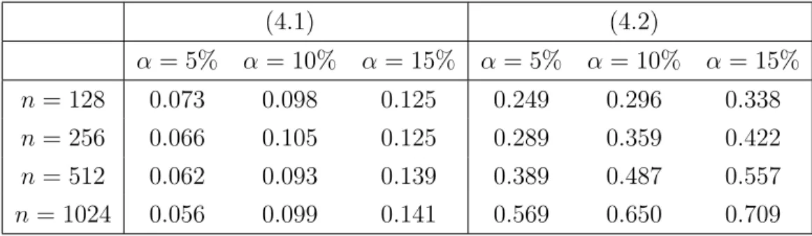
Example 4.1: Testing for a constant spectral density. In order to investigate the testing problem (2.3) we consider the models

X_t = Z_t (4.1)

Xt = Zt+1 5Zt+1, (4.2)

corresponding to null hypothesis and alternative, respectively. Here {Z_t}_t∈Z is a Gaussian white noise process with variance σ² = 1. Note that for model (4.2) the spectral density is given by

f(λ) = _2π^{1 26}₂₅ +²₅cos(λ)

. In Table 1 we show the rejection probabilities of the test (2.11) for var- ious sample sizes, where the asymptotic variance has been estimated by (2.12). We observe a rather accurate approximation of the nominal level and reasonable rejection probabilities under the alternative.

Simulations of other scenarios showed a similar picture and are not displayed for the sake of brevity.

(4.1) (4.2)

α = 5% α = 10% α= 15% α= 5% α= 10% α= 15%

n = 128 0.073 0.098 0.125 0.249 0.296 0.338

n = 256 0.066 0.105 0.125 0.289 0.359 0.422

n = 512 0.062 0.093 0.139 0.389 0.487 0.557

n = 1024 0.056 0.099 0.141 0.569 0.650 0.709

Table 1: Rejection probabilities of the test (2.11) for the hypothesis of a constant spectral density under the null hypothesis and alternative.

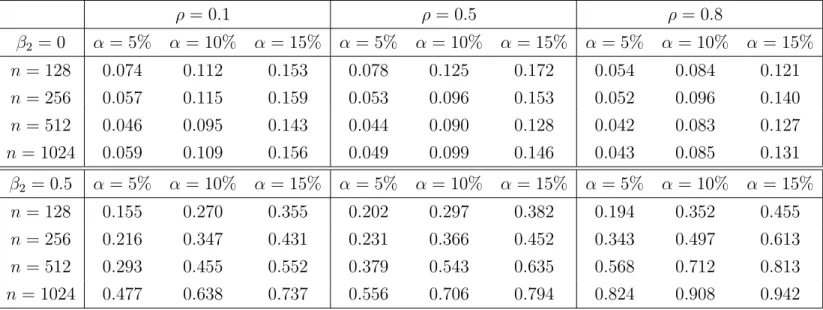
Example 4.2: Comparing spectral densities of stationary time series. In this example we study the testing problem (3.1) in the casem= 2, where the stationary time series is given by{(X1,t, X2,t)}t∈Z

with

X_1,t = Z_1,t−β₁Z1,t−1−β₂Z1,t−2

X_2,t = Z_2,t−β₁Z_2,t−1

Here β₁ = 0.8, and {(Z_1,t, Z_2,t)^T}t∈Z is an independent centered stationary Gaussian process with covariance matrix

Σ = 1 ρ ρ 1

! ,

and the choice β₂ corresponds to either the null hypothesis of equal spectral densities (β₂ = 0) or to the alternative (β₂ 6= 0). In Table 2 we present the rejection probabilities of the test (3.8) for various sample sizes where we used the variance estimate (3.7). We observe again that the nominal level is well approximated and that the alternatives are clearly detected in all cases. It is interesting to note that the power of the test is increasing with the correlationρ of the Gaussian process. A similar observation was also made by Dette and Paparoditis (2009) for a test based on a kernel estimate of the spectral density matrix.

In the present situation the empirical observations can be explained by the asymptotic theory presented in Section 3. First, note that under the alternative the probability of rejecting the null hypothesis of equal spectral densities by the test (3.8) is approximately given by

(4.3) P√

n D_n ˆ

τ_D,H0 > u1−α

≈Φ√ nD²

τ_D² −u1−α

τ_D²_,H0 τ_D²

≈Φ√ nD²

τ_D²

ρ= 0.1 ρ= 0.5 ρ= 0.8

β₂ = 0 α= 5% α= 10% α= 15% α= 5% α = 10% α = 15% α = 5% α= 10% α= 15%

n = 128 0.074 0.112 0.153 0.078 0.125 0.172 0.054 0.084 0.121

n = 256 0.057 0.115 0.159 0.053 0.096 0.153 0.052 0.096 0.140

n = 512 0.046 0.095 0.143 0.044 0.090 0.128 0.042 0.083 0.127

n= 1024 0.059 0.109 0.156 0.049 0.099 0.146 0.043 0.085 0.131

β2 = 0.5 α= 5% α= 10% α= 15% α= 5% α = 10% α = 15% α = 5% α= 10% α= 15%

n = 128 0.155 0.270 0.355 0.202 0.297 0.382 0.194 0.352 0.455

n = 256 0.216 0.347 0.431 0.231 0.366 0.452 0.343 0.497 0.613

n = 512 0.293 0.455 0.552 0.379 0.543 0.635 0.568 0.712 0.813

n= 1024 0.477 0.638 0.737 0.556 0.706 0.794 0.824 0.908 0.942

Table 2: Simulated rejection probabilities of the test (3.8) for the hypothesis (3.1) of equal spectral densities.

where Φ denotes the distribution function of the standard normal distribution andτ_D,H²

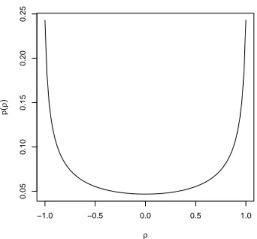
0 andτ_D² are the asymptotic variances under the null hypothesis and alternative, respectively [see equations (3.5) and (3.6)]. This shows that the power is increasing with the ratio D²/τ_D². In Figure 1 we display the ratio

ρ→p(ρ) = D²(ρ) τ_D(ρ) (4.4)

as a function ofρ∈[−1,1] and we observe that the asymptotic power (4.3) is an increasing function of

|ρ|. This confirms our empirical observations in Table 2.

5 Conclusions

In this paper we have illustrated an alternative concept for constructing tests for nonparametric hy- potheses in stationary time series with a linear representation of the form (2.1). Our approach is based on an estimate of theL²-distance between the spectral density matrix and its best approximation under the null hypothesis and does not require the specification of a smoothing parameter. The test statistic is constructed from simple estimates of integrated components of the spectral density matrix and follows an asymptotic normal distribution. For the sake of a clear presentation and brevity we have restricted ourselves to the problem of testing for a constant spectral density matrix and to the comparison of the spectral densities of several correlated time series.

We conclude this paper with a few remarks on generalizations of our approach. First, the generalization of the approach to other hypotheses is obvious, if we consider the minimal distance

M² = min nZ π

−π

tr{(f(λ)−g(λ))(f(λ)−g(λ))^∗}dλ | g ∈ F_H0o , (5.1)

−1.0 −0.5 0.0 0.5 1.0

0.050.100.150.200.25

ρ

p(ρ)

Figure 1: The function p(ρ) defined in (4.4) for various values of ρ

whereF_H0 denotes the set of all spectral densities satisfying the null hypothesis under consideration. In most cases this minimal distance can be given explicitly in terms of integrals of elements of the spectral density matrix over the full frequency domain [−π, π]. Typical examples include the problem of no correlation and separability. The first problem corresponds to the hypothesis

H₀ :f_ij(λ) = 0, 1 ≤i < j≤m

in the frequency domain. In this case, it is easy to see that the minimum in (5.1) is given by M² = 2 X

1≤i<j≤m

Z π

−π

|fij(λ)|²dλ

which can be estimated easily using the approach described in Sections 2 and 3. The (appropriately standardized) test statistic is asymptotically normal distributed and it only remains to estimate the asymptotic variance under the null hypothesis. The second example corresponds to the hypothesis of separability

H₀ :f(λ) = Σf₀(λ)

[see e.g. Matsuda and Yajima (2004)], where Σ denotes a positive definite matrix and f₀(λ) is a real- valued function which is integrable on [−π, π]. Without loss of generality one can take Σ to be the variance of the process {X_t}t∈Z, which gives

f₀(λ) = 1 mtr

f(λ)V_Σ⁻¹

= 1 m

m

X

i=1

f_ii(λ) Rπ

−πf_ii(λ)dλ

with V_Σ = diag(σ₁², . . . , σ²_m) being the diagonal matrix whose entries are the variances of X_t,i [see also Eichler (2008)]. Using the same approach as in Section 2 it can be shown that the distance in (5.1)

becomes minimal for

Σ₀ = Rπ

−πf(λ)f₀(λ)dλ Rπ

−πf₀²(λ)dλ , which gives

M² = Z π

−π

tr(f(λ)f^∗(λ))dλ− tr((Rπ

−πf(λ)f₀(λ)dλ)(Rπ

−πf(λ)f₀(λ)dλ)^∗) Rπ

−πf₀²(λ)dλ .

This quantity can also be estimated easily by the methods described in the previous paragraphs. Other hypotheses can be treated similarly, and the concept presented here is applicable as soon as the minimal distance can be represented as a functional of the spectral density matrix.

Second, the restriction to Gaussian innovations was made throughout this paper in order to keep the arguments simple. In fact, similar results can be derived for arbitrary linear processes of the form (2.1), as long as the sequence of innovations{Z_t}t∈Zis independent identically distributed withE[Z_t] = 0 and existing moments of eighth order. Note however that the simple form of the variances τ_M²2 and τ_D²2 in both theorems is due to special properties of the normal distribution and that cumulants of higher orders show up in general. For example, if we are in the situation of Theorem 2.1 (and in the one-dimensional case m= 1), we obtain a central limit theorem √

n(T_n−M²)−→N^D (0, τ²_M2) with variance τ²_M2 = 20π

Z π

−π

f⁴(λ)dλ−16 Z π

−π

f(λ)dλ Z π

−π

f³(λ)dλ+ 4 π

Z π

−π

f(λ)dλ 2Z π

−π

f²(λ)dλ (5.2)

+q1 π

Z π

−π

f(λ)dλ2

−2 Z π

−π

f²(λ)dλ2

,

whereq =κ₄/σ⁴ andκ₄ =E[Z_t⁴]−3σ² denotes the fourth cumulant ofZ_t. This term coincides withτ_M²2

if Zt is normally distributed, as we haveκ4 = 0 in this case. Moreover, under the null hypothesis of a constant spectral density the asymptotic variance in (5.2) does also not depend on the fourth cumulant.

A similar phenomenon can be observed for the tests proposed by Eichler (2008) for a general class of hypotheses [see Dette and Hildebrandt (2010)].

6 Appendix: some technical details

In this section, we show the estimates (2.8) and (2.9) which are the main ingredients for the proof of both Theorem 2.1 and 3.1. To this end, let R_n(λ_k) = I_n(λ_k)−I˜_n(λ_k) denote the differences in (2.8), which by a standard argument [see Brockwell and Davis (1991), p. 347] can be represented as

R_n(λ_k) = ψ(e^−iλk)J_n,z(λ_k)Y_n(λ_k) +ψ(e^−iλk)J_n,z(λ_k)Y_n(λ_k) +|Y_n(λ_k)|² (6.1)

= R_n,1(λ_k) +R_n,2(λ_k) +|Y_n(λ_k)|²,

where we have used the notation

ψ(e^−iλ) =

∞

X

j=−∞

ψ_je^−iλj

U_n,j(λ) =

n−j

X

t=1−j

Z_te^−iλt−

n

X

t=1

Z_te^−iλt

Y_n(λ) = 1

√n

∞

X

j=−∞

ψ_je^−iλjU_n,j(λ) (6.2)

and the quantitiesR_n,1 andR_n,2 are defined in an obvious way. Using the symmetry of the periodogram [and ignoring boundary effects] it is our aim to show

√1 n

bⁿ₂c

X

k=−bⁿ⁻¹₂ c

R_n(λ_k)

=o_P(1) (6.3)

in order to obtain (2.8). It is well known [see Brockwell and Davis (1991)] that E|Y_n(λ_k)|² ≤E(|Y_n(λ_k)|⁴)¹² =O(n⁻¹),

(6.4)

which yields the assertion for the third term in (6.1). The remaining two terms can be treated similarly, so for the sake of brevity onlyR_n,1(λ_k) is considered here. This quantity can be decomposed as follows:

First we set

Y_n(λ_k) = 1

√n

−1

X

l=−∞

ψ_le^−iλklU_n,l(λ_k) + 1

√n

∞

X

l=0

ψ_le^−iλklU_n,l(λ_k) (6.5)

= H_n⁻(λ_k) +H_n⁺(λ_k),

where the last identity defines the expressions H_n⁻ and H_n⁺. By definition we have λ_k = ^2πk_n , so a straightforward calculation yields the representation

H_n⁺(λ_k) = 1

√n

∞

X

l=0 l

X

r=1

ψ_l(Zr−l−Zn+r−l)e^−iλkr, (6.6)

H_n⁻(λ_k) = 1

√n

−1

X

l=−∞

0

X

r=1+l

ψ_l(Zn+r−l−Zr−l)e^−iλkr. Setting

R⁺_n,1 =

bⁿ₂c

X

k=−bⁿ⁻¹₂ c

ψ(e^−iλk)J_n,z(λ_k)H_n⁺(λ_k)

= 1 n

bⁿ₂c

X

k=−bⁿ⁻¹c

∞

X

j=−∞

∞

X

l=0 l

X

r=1 n

X

t=1

ψ_jψ_lZ_t(Zr−l−Zn+r−l)e^{−iλk(j+t−r)}

and similarly

R⁻_n,1 =

bⁿ₂c

X

k=−bⁿ⁻¹

2 c

ψ(e^−iλk)J_n,z(λ_k)H_n⁻(λ_k)

we are left to show that both n^−1/2E|R⁺_n,1| and n^−1/2E|R⁻_n,1|converge to zero, and we restrict ourselves to the proof of the first claim. Note for any fixed two integersj and r that the relation

bⁿ₂c

X

k=−bⁿ⁻¹₂ c

e^{−iλk(j+t−r)}=

(n, t =r−j modn 0, otherwise

(6.7)

holds, from which we conclude R⁺_n,1 =

∞

X

j=−∞

∞

X

l=0 l

X

r=1

ψ_jψ_lZ_t^∗(Zr−l−Zn+r−l),

wheret^∗ =t(r, j) is the unique t∈ {1, . . . , n}, such thatt=r−j mod n holds. Therefore E|R⁺_n,1| ≤ 2σ²

∞

X

j=−∞

∞

X

l=0 l

X

r=1

|ψj||ψl| ≤2σ²

∞

X

j=−∞

|ψj|

∞

X

l=−∞

|l| |ψl|=O(1),

where we have used condition (2.6) for the last estimate. Analogously, the estimate E|R⁻_n,1| = O(1) follows, and a similar argument for the sum involving R_n,2(λ_k) yields assertion (2.8).

We now turn to the proof of estimate (2.9). From (6.3), the Cauchy-Schwarz inequality and the symmetry of the periodogram we have

E

√1 n

bⁿ₂c

X

k=1

I_n(λ_k)I_n(λk−1)−I˜_n(λ_k) ˜I_n(λk−1) (6.8)

= E

1 2√ n

bⁿ

2c

X

k=−bⁿ⁻¹

2 c

I_n(λ_k)I_n(λk−1)−I˜_n(λ_k) ˜I_n(λk−1)

+o(1)

= E

1 2√ n

bⁿ₂c

X

k=−bⁿ⁻¹₂ c

I˜n(λk)Rn(λk−1) + 1 2√ n

bⁿ₂c

X

k=−bⁿ⁻¹₂ c

I˜n(λk−1)Rn(λk)

+o(1).

Once we have shown the claim E 1

√n

bⁿ₂c

X

k=−bⁿ⁻¹₂ c

I˜_n(λ_k)R_n(λk−1)2

=o(1) (6.9)

and an analogous estimate with λ_k replaced by λk−1 and vice versa, (2.9) follows.