Deep Controlled Source Electromagnetics for Mineral Exploration: A Multidimensional Validation Study in
Time and Frequency Domain
Inaugural-Dissertation
zur Erlangung des Doktorgrades
der Mathematisch-Naturwissenschaftlichen Fakultät der Universität zu Köln
vorgelegt von Wiebke Mörbe aus Freiburg im Breisgau
Köln, 2020
Tag der mündlichen Prüfung: 25.11.2019
Abstract
The focus of this thesis is the derivation of an independent multidimensional resistivity model utilising land based controlled source electromagnetics (CSEM) with resolution to conductive structures down to 1 km depth. Data is evaluated in both, time and frequency domain. Since the resistivity distribution is strongly multidimensional, besides conven- tional 1D inversion methods, 2D inversion techniques are applied to the dataset.
The objective of the BMBF funded DESMEX (Deep Electromagnetic Sounding for Min- eral Exploration) project is the development of an electromagnetic exploration system which can be used for the detection and assessment of deep mineral resources. In order to obtain a high data coverage as well as a high spatial and depth resolution, airborne and ground based methods are combined in a semi-airborne concept. In the framework of the DESMEX project, the University of Cologne conducted large scale ground based long off- set transient electromagnetic (LOTEM) measurements along an 8.5 km long transect in a former mining area in eastern Thuringia, Germany. Within the LOTEM validation study, an independent multidimensional resistivity model of the survey area was derived, which serves as a reference model for the semi-airborne concept developed within DESMEX and is eventually integrated into a final mineral deposition model. Utilising in total 6 trans- mitters in broadside configuration, data at 170 electric field stations were recorded during two large scale LOTEM surveys. In addition, a full component magnetic field dataset was acquired with SQUID sensors using a dense station spacing along the transect. For a preliminary evaluation, conventional 1D techniques are applied to the dataset. The individual switch on transients of the electric field can be explained by a 1D approach, the obtained models however indicate a strong multidimensional subsurface with rather large variations in resistivity. For further interpretation, the LOTEM data is analysed in frequency domain. Obtained 1D and 2D inversion models of the electric field component in frequency domain are in a good agreement with the time domain results. Subsequently, a joint multidimensional inversion of the full dataset in frequency domain was carried out, including electric and magnetic field data. Derived 2D inversion models are discussed in terms of sensitivities and resolution capabilities. Shallow high conductive structures are well comparable to inversion results from other conducted reconnaissance surveys and the semi-airborne CSEM model. The dominant conductivity structures can be linked to the occurrence of Silurian graptolite shales.
i
Kurzzusammenfassung
Ziel dieser Arbeit ist die Ableitung eines unabhängigen Leitfähigkeitsmodells mit Hilfe von bodengebundenen Controlled Source Electromagnetic (CSEM) Messungen, welches Leitfähigkeitsstrukturen bis in 1 km Tiefe auflösen kann. Gemessene Daten werden sowohl im Frequenzbereich als auch im Zeitbereich ausgewertet. Da die Leitfähigkeitsverteilung deutliche Eigenschaften von Mehrdimensionalität aufweist, werden neben 1D Auswerteme- thoden auch 2D Inversionsalgorithmen angewandt.
Ziel des BMBF geförderten DESMEX Projektes (Deep Electromagnetic Sounding for Min- eral Exploration) ist die Entwicklung eines elektromagnetischen Explorationsverfahrens, welches für die Detektion und Bewertung tiefer mineralischer Lagerstätten eingesetzt wer- den kann. Um sowohl eine hohe flächenhafte Datenabdeckung als auch eine hohe räum- liche und vertikale Auflösung zur ermöglichen, werden bodengebundene und luftgestützte Systeme in einem Semi Airborne Konzept kombiniert. Im Rahmen des DESMEX Pro- jektes führte die Universität zu Köln bodengebundene Long Offset Transiente Elektro- magnetische (LOTEM) Messungenen entlang eines 8.5 km langen Profils in einem ehema- ligen Abbaugebiet in Ostthüringen, Deutschland durch. Im Rahmen der LOTEM Vali- dierungsstudie soll ein mehrdimensionales Leitfähigkeitsmodell abgeleitet werden, das als Referenzmodell für das neue Semi Airborne Konzept dient und in ein gemeinsames Lager- stättenmodell eingebunden wird. Im Rahmen von zwei großskaligen LOTEM Messkam- pagnen wurden unter Nutzung von 6 Sendern in Broadside Konfiguration Daten an 170 elektrischen Feld Stationen aufgezeichnet. Zusätzlich wurden die 3 Komponenten des Magnetfeldes mit dichtem Stationsabstand entlang des Profils mit einem SQUID Mag- netometer aufgenommen. Als ersten Auswerteansatz wurden konventionelle 1D Inver- sionsroutinen auf den Datensatz angewendet. Die aufgezeichneten Switch-On Transien- ten des elektrischen Feldes können mit einer 1D Leitfähigkeitsverteilung erklärt werden.
Die abgeleiteten 1D Leitfähigkeitsmodelle deuten allerdings auf eine deutlich mehrdi- mensionale Leitfähigkeitsverteilung mit starken Kontrasten entlang des Profils hin. Für eine weiterführende Interpretation wurde der Datensatz im Frequenzbereich ausgewertet.
Die abgeleiteten 1D und 2D Inversionsmodelle im Frequenzbereich stimmen gut mit den Ergebnissen im Zeitbereich überein. Daher wurden im Anschluss eine gemeinsame, mehrdimensionale Inversion des elektrischen und magnetischen Datensatzes durchgeführt.
Sensitivitäten und Auflösungseigenschaften der abgeleitete 2D Modelle in Zeit- und Fre-
iii
quenzbereich werden diskutiert. Oberflächennahe Leitfähigkeitsstrukturen stimmen gut
mit den Inversionsergebnissen von luftgestützten Voruntersuchungen und dem Semi Air-
borne Modell überein und korrelieren mit dem Auftreten silurischer Schwarzschiefer.
Contents
List of Figures ix
List of Tables xiii
1. Introduction 1
2. The LOTEM Method 5
2.1. Electrical Conduction Mechanisms . . . . 7
2.2. Maxwell Equations . . . . 8
2.2.1. Plane Wave Solution for a Uniform Conducting Halfspace . . . . 9
2.2.2. Step Excitation Solution for a Uniform Conducting Halfspace . . . 10
2.3. HED Solution for a Uniform Conducting Halfspace . . . 10
2.3.1. HED Solution in Frequency Domain . . . 11
2.3.2. Near Field Approximation FD . . . 12
2.3.3. Far Field Approximation FD . . . 13
2.3.4. HED Solution in Time Domain . . . 14
2.3.5. Near Field Approximation TD . . . 15
2.3.6. Far Field Approximation TD . . . 16
2.4. Practical Exploration Depth . . . 16
2.5. Summary . . . 17
3. Inversion Theory 19 3.1. The Inverse Problem . . . 19
3.2. Well and Ill Posed Problems . . . 20
3.3. The Unconstrained Linearised Problem . . . 21
3.4. Gauss Newton and Steepest Descent Method . . . 22
3.5. Constrained Occam Inversion . . . 23
3.5.1. The Regularization Parameter . . . 25
3.6. Marquardt-Levenberg Algorithm . . . 25
3.6.1. SVD . . . 25
3.6.2. Eigenvalue Analysis . . . 26
3.6.3. Importance and BTSV . . . 27
3.6.4. Equivalent Models . . . 27
v
3.7. Calibration Factor . . . 28
3.8. Parameter Transformation . . . 28
4. The DESMEX Project 31 4.1. Detecting Deep Structures with LOTEM . . . 32
4.2. Geology of the Survey Area . . . 33
4.3. Petrophysical Measurements . . . 36
4.4. Further Geophysical Investigations . . . 37
4.5. Summary . . . 38
5. Field Setup 41 5.1. Transmitter System . . . 43
5.2. Receiver Systems and Sensors . . . 45
5.3. Summary . . . 47
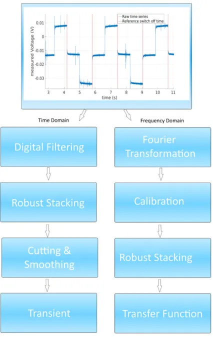
6. Data Processing 49 6.1. Time Domain Processing . . . 52
6.1.1. Preprocessing: Switching Times . . . 52
6.1.2. Digital Filtering . . . 53
6.1.3. Cutting and Stacking . . . 55
6.1.4. Application of Hanning Window . . . 56
6.1.5. The System Response . . . 57
6.1.6. Data Representation . . . 59
6.2. Frequency Domain Processing . . . 61
6.2.1. Discrete Fourier Transform . . . 62
6.2.2. Application of Calibration Functions . . . 64
6.2.3. Calculation of Robust Transfer Functions . . . 65
6.2.4. Data Representation in FD . . . 66
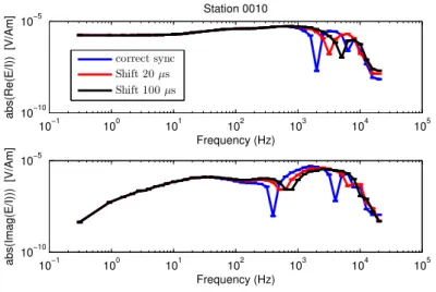
6.3. Effects of Synchronisation Errors . . . 69
6.4. The Dataset . . . 71
6.5. Summary . . . 76
7. 1D Inversion of the Dataset 79 7.1. 1D Inversion in Time Domain . . . 79
7.1.1. Inversion of Switch Off Transients . . . 80
7.1.2. Occam Inversion and Datafit for Tx 8 . . . 80
7.1.3. 1D Inversion Results of E-Field Data . . . 82
7.1.4. Influence of 2D Conductivity Structures . . . 83
7.1.5. Magnetic Field Data . . . 85
7.2. 1D Inversion Models in TD and FD . . . 86
7.2.1. Synthetic Resolution Study . . . 88
7.3. The Influence of IP . . . 90
7.4. Summary . . . 91
8. Synthetic 2D Modelling Studies 93 8.1. The MARE2DEM Algorithm . . . 94
8.1.1. Calculation of Sensitivities . . . 95
8.1.2. Fast Occam Inversion . . . 95
Contents vii
8.1.3. Bounds on Model Parameters . . . 96
8.2. Synthetic Tests with MARE2DEM . . . 98
8.2.1. Validation of the FD Response . . . 99
8.2.2. Creation of the Inversion Mesh . . . 101
8.2.3. Influence of Topography . . . 103
8.2.4. Influence of the Starting Model . . . 105
8.2.5. Influence of Smoothing Parameters . . . 106
8.2.6. Resolution of Different Field Components . . . 106
8.2.7. Resolution of Resistive Structures . . . 108
8.2.8. Error Settings . . . 109
8.2.9. Inversion of Imaginary and Real Part . . . 111
8.2.10. Synthetic Tests in Time Domain . . . 113
8.2.11. Validation of the TD Response . . . 113
8.2.12. Sensitivities in TD and FD . . . 114
8.3. Summary . . . 116
9. 2D Inversion of Field Data 119 9.1. 2D Inversion of Field Data in FD . . . 119
9.1.1. Single Component Inversion . . . 120
9.1.2. The B x Component . . . 123
9.1.3. The CSEM Validation Model . . . 124
9.2. 2D Inversion of E x in Time Domain . . . 128
9.2.1. Inversion of Late Time E x Data . . . 129
9.2.2. Inversion of E x Data . . . 130
9.3. Summary . . . 132
10.Validation of Inversion Results 135 10.1. Comparison with Geophysical Results . . . 136
10.2. Comparison with Geology . . . 139
10.3. Summary . . . 140
11.Conclusion and Outlook 143 Bibliography 147 Appendix 155 A. Survey Setup . . . 155
B. Data Processing . . . 170
C. Synthetic 2D Studies . . . 187
D. 2D Inversion . . . 191
List of Figures
2.1. LOTEM Setup in Broadside Configuration . . . . 5
2.2. Transmitter Duty Cycle and Response . . . . 6
2.3. Field Components . . . 11
3.1. Minimisation Methods . . . 23
4.1. The DESMEX System . . . 32
4.2. Target Response Deep Conductor . . . 33
4.3. Geological Overview and HEM Results . . . 34
4.4. Geological Map, Cross Section and LOTEM Profile . . . 35
4.5. Petrophysics in Schleiz . . . 37
5.1. Map LOTEM Validation Study . . . 42
5.2. Transmitter Setup . . . 44
5.3. Transmitter Ramp . . . 45
5.4. Comparison of Receiver System . . . 46
5.5. SQUID vs. Induction Coil . . . 47
6.1. Flowchart Data Processing . . . 51
6.2. Selecting Switching Times . . . 53
6.3. Three-Point Filter . . . 54
6.4. QQ Plot . . . 56
6.5. Smoothed Transient . . . 57
6.6. System Response . . . 58
6.7. Transient Response . . . 60
6.8. Power Spectrum . . . 62
6.9. Influence of Window Length . . . 63
6.10. 450 Hz Noise . . . 64
6.11. Calibration Function . . . 65
6.12. Transfer Function E x . . . 66
6.13. Transfer Functions B x ,B y . . . 68
6.14. Transfer Function B z . . . 68
6.15. Effects of Synchronisation Errors . . . 69
ix
6.16. Time Shift in Frequency Domain . . . 70
6.17. Linear Drift in Time Domain . . . 70
6.18. Transmitter Receiver Geometry . . . 72
6.19. Voltages Tx 8 TD E-Fields . . . 72
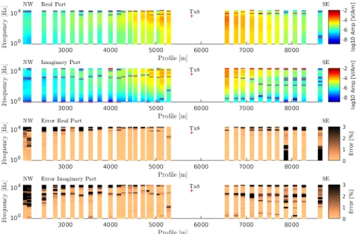
6.20. Voltages Tx 8 FD E-Fields . . . 73
6.21. Voltages Tx 8 FD B x ,B y -Fields . . . 74
6.22. Voltages Tx 8 FD B z -Fields . . . 75
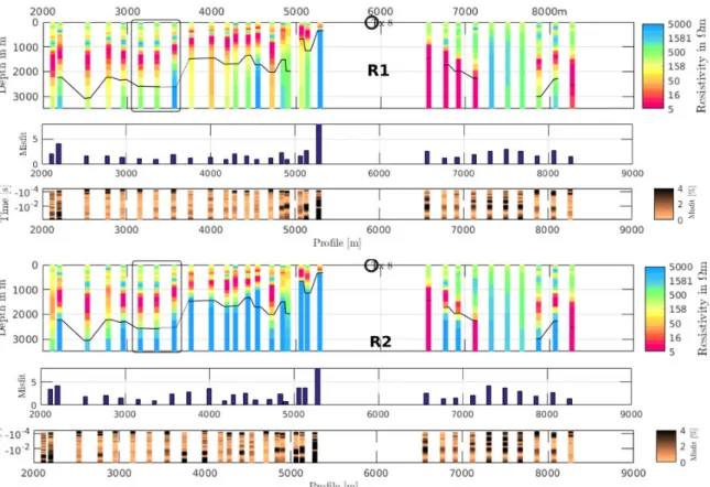
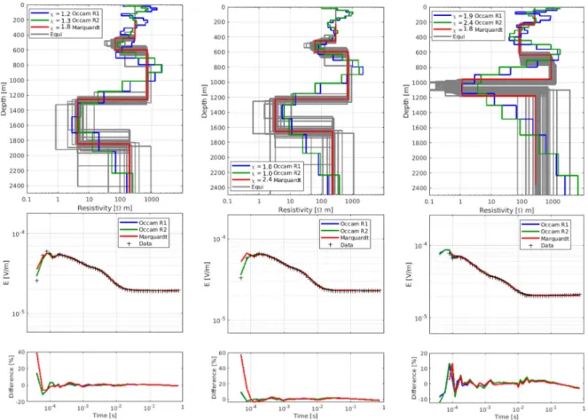
7.1. Inversion of Switch On and Switch Off Transients . . . 81
7.2. Inversion Occam R1 and R2 . . . 82
7.3. Inversion Results for 3 Selected Stations . . . 83
7.4. 1D Inversion of Electric Field Data . . . 84
7.5. Occam R1 Tx 3,Tx6 Rx 18 Inversion Results . . . 84
7.6. 1D inversion of a 2D dataset . . . 85
7.7. 1D Inversion of E-and B-Field Data . . . 86
7.8. Comparison of 1D Inversion Results in TD and FD . . . 87
7.9. Eigenvalue Analysis . . . 89
7.10. IP Effects in TD and FD . . . 91
8.1. Fast Occam Approach . . . 97
8.2. Positioning of Transmitters . . . 98
8.3. FD Dipole Response . . . 99
8.4. Validation of Extended Dipole (FD) . . . 100
8.5. Dependency of Response to Receiver Grouping . . . 101
8.6. Inversion Mesh . . . 102
8.7. Grid Testing . . . 103
8.8. Influence of Topography . . . 104
8.9. Influence of Starting Model . . . 105
8.10. Influence of Smoothing Parameters . . . 106
8.11. Inversion of Different Components . . . 107
8.12. Resolution of Resistive Structures . . . 109
8.13. Influence of Error Settings . . . 110
8.14. Inversion of Imaginary and Real Part . . . 111
8.15. Sensitivity Distribution FD . . . 112
8.16. Validation of Extended Dipole (TD) . . . 114
8.17. Time and Frequency Domain Sensitivities . . . 115
8.18. Time and Frequency Domain Inversion . . . 116
9.1. Inversion Results of B y , B z and E x . . . 121
9.2. Data Fit for Inversion Results of B y , B z and E x . . . 122
9.3. Inversion Results of B y , B z and E x for the Upper 400 m. . . 123
9.4. The B x Component . . . 124
9.5. CSEM Validation Model . . . 125
9.6. Data Fit for the Joint Inversion Result . . . 126
9.7. Forward Model without Deep Anomaly . . . 127
9.8. DC Level Inversion . . . 129
9.9. Inversion of E x in TD and FD . . . 131
9.10. Data Fit of E x in TD and FD . . . 132
List of Figures xi
10.1. Comparison of Inversion Results from Different Methods . . . 136
10.2. Comparison between the Validation Model and Semi-Airborne Model . . . 138
10.3. Comparison of CSEM and Airborne Inversion Models with Geology . . . . 140
List of Tables
2.1. Variables and Constants . . . . 7 9.1. Data Fit between Models from Individual Components . . . 121 9.2. RMS of the Validation Model . . . 125
xiii
CHAPTER 1
Introduction
The focus of this thesis is the derivation of an independent multidimensional resistivity model utilizing land based controlled source electromagnetics (CSEM) for the validation of a newly developed semi-airborne concept for deep mineral exploration applications.
Hereby, acquired CSEM data is analysed in both, time domain (TD) and frequency do- main (FD) with the focus on deep conductive structures.
Ore mineralisation can increase the electrical conductivity in the subsurface significantly (e.g. Airo (2015); Spagnoli et al. (2016)). Electromagnetic methods, which gain informa- tion about the electrical conductivity properties of the subsurface, play an essential role for mineral exploration. There exists multiple electromagnetic studies successfully applied to mineral exploration applications in the last decades, either airborne (Witherly, 2000) or ground based (Strack et al., 1990), and EM is nowadays an established tool for mineral exploration. The depth extension of economic mineral deposits in Germany is poorly known. On the other hand, the exploitation of strategic important minerals is nowadays feasible for depth larger than 1 km. Therefore an efficient method is needed to evaluate the depth extension of the deposits. In the framework of the joint DESMEX project (Deep electromagnetic sounding for mineral exploration), funded by the German Federal Min- istry of Education and Research (BMBF), a novel concept is developed (Smirnova et al., 2019b; Nittinger et al., 2017; Schiffler et al., 2017), where airborne and ground based EM methods are combined. The semi-airborne technique aims at deep electromagnetic explo- ration down to 1 km. Having the advantage, that airborne electromagnetic measurements can cover a large area rapidly, whereas ground based methods deliver complimentary in- formation, a combination of both techniques provide a powerful tool to explore the depth extension of potential deposits for strategic resources. Within the validation study, long offset transient electromagnetic (LOTEM) measurements were performed in the survey area with the aim to derive an independent multidimensional resistivity model, which serves as a reference model for the semi-airborne concept and is eventually integrated in a final mineral deposition model.
1
The LOTEM method is a controlled source electromagnetic method in time domain and was predominantly advanced by Strack et al. (1990) and further developed at the Uni- versity of Cologne (UoC) in the last decades. A theoretical description of LOTEM and CSEM methods in general can be found in various textbooks (e.g. Kaufman and Keller (1983); Nabighian and Macnae (1991)). LOTEM utilizes typically a horizontal electrical dipole (HED) with cable length between 1-2 km as transmitter and multi-component EM receiver stations at offsets ranging from 1 km up to several km from the source. As source signal, a square wave with alternating polarisation is used. Switching times and corre- sponding transient length used for LOTEM applications range typically between 10 −4 s up to few decades of seconds. Depending on the geometry, the time range and the resis- tivity distribution of the subsurface, investigation depth between several tens of meters up to several decades of km can be reached (Ziolkowski et al., 2007; Haroon et al., 2015).
Recent applications of time domain CSEM at the UoC comprise e.g. applications of LOTEM in a marine environment for the detection of a groundwater aquifer (Lippert, 2015). Haroon (2016) developed a novel differential electrical dipole method for marine applications. Resistivity distributions were reconstructed typically by the application of 1D inversion routines and large scale 2D forward modelling studies. However, if the geology is rather complex, the electrical resistivity distribution can be strongly multidi- mensional. Trial and error forward modelling studies are time consuming and not efficient for the deviation of complex large scale models.
Multidimensional time domain modelling algorithms were presented by few authors, e.g.
Martin (2009); Commer (2003); Oldenburg et al. (2012). However, open source inversion tools for time domain land based CSEM suitable for long offset applications are still not commonly available and not routinely utilized. Yogeshwar (2014) applied the 2D inver- sion algorithm SINV developed by Martin (2009) to an in-loop TEM dataset for shallow geomorphological applications. However, for the given LOTEM dataset presented in this thesis, the application of the SINV algorithm did not lead to satisfying results due to convergence and stability issues for large resistivity contrasts. In addition, for finite dif- ference algorithms like SINV, the implementation of topography is not straight forward and results in a higher demand of computational resources.
On the other hand, for frequency domain CSEM applications, a range of open source fre- quency domain codes exists, which are tested for onshore galvanic dipole configurations (Key and Ovall, 2011; Grayver et al., 2013). From a theoretical point of view, the time domain and frequency domain approach is related over a Fourier transformation (Streich, 2016). However, advantages of the CSEM time domain methods in contrary with the conventional CSEM frequency domain method were advertised by several authors, e.g.
Zhdanov (2010) and Strack (1992). One of the main reasons is the possibility to measure the transient step response of the earth in absence of the primary field (Streich, 2016), i.e.
after the transmitter is switched off and in the case of land based application after the
arrival of the air wave. The measurement setup is for both, time and frequency domain
CSEM methods similar. Typically a HED is utilized as a source and a rectangular shaped
signal is transmitted. For time domain applications the transient response after current
switch off or switch on is evaluated. In frequency domain, transfer functions between
the source current and the measured EM field responses for the transmitted fundamental
3 frequency and its odd harmonics are evaluated. If an analysis of the data in frequency and time domain is possible, depends therefore mainly on the capabilities of the used instrumentation.
The application of 1D inversion algorithms are not suitable for the collected LOTEM dataset and the time domain transients are distorted by induced polarization effects.
Hence, for the derivation of a deep subsurface model a more methodological aspect of CSEM application is investigated. In the framework of this thesis, the LOTEM dataset was evaluated in both, time and frequency domain. As the measurement equipment of the University of Cologne was so far only validated for time domain applications, both, transmitter and receiver systems were tested for an evaluation in frequency domain. Res- olution studies for different data representations with the focus on deep conductive layers were performed. Haroon (2016) studied differences in the resolution capabilities of switch on and switch off transients. In the framework of this thesis, sensitivities towards deep conductors (and resistors) are studied in both domains and for different data representa- tions. Whereas for an isotropic earth (Kaufman and Keller, 1983) no physical difference regarding the inductive response is present between those data representations, the rela- tive contribution of the inductive earth response and time independent background DC field may vary. Under consideration of an absolute and relative noise floor, this results in different resolution capabilities of time domain switch on and switch off transients as well as frequency domain transfer functions. Additionally, induced polarization is affecting the electromagnetic response in both domains differently. This thesis therefore aims not for a general recommendation of the advantages and disadvantages of one method over the other. However, it is demonstrated that under the given circumstances with respect to the survey design, depth of investigation and instrumentation, an interpretation of data in both domains is feasible and leads to comparable results.
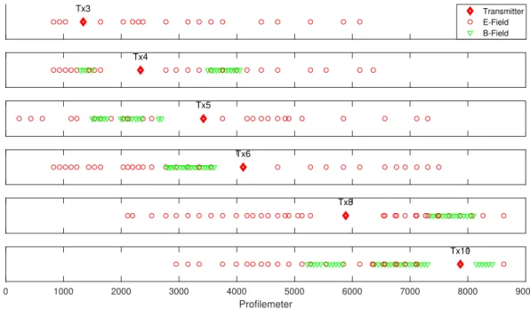
As a test area for the new semi-airborne method within DESMEX, a former antimony mining area in the Thuringian Slate Mountains, Germany was chosen. Due to its rather high resistivity (Costabel and Martin, 2019) and restricted extension (Schlegel and Wiefel, 1998), the antimony mineralisation itself can not be detected with electromagnetic meth- ods. However, in the survey area graphitised black shales are present, which exhibit a high electrical conductivity contrast to the surrounding host rock material and therefore deliver an applicative target for electromagnetic induction methods. Located in a heav- ily faulted and deformed Antiform structure, the geological setting of the survey area is rather complex. Where the resistivity distribution of the shallow subsurface can be constrained by either geological and available borehole information or shallow geophys- ical investigation methods (e.g. airborne electromagnetics, radio-magnetotellurics), the deep structures remain unknown. In order to validate the newly developed semi-airborne concept down to depth of 1 km, a large scale ground based LOTEM survey along an 8.5 km long transect was carried out. To facilitate fast data acquisition in the framework of the LOTEM validation study and evaluate potential additional equipment resources for future time domain CSEM applications, magnetotelluric data loggers provided by the geophysical instrument pool Potsdam (GIPP) were tested for time domain applications.
Next to the acquisition of electric field data, the full magnetic field response was measured
at a dense spacing utilizing low temperature SQUID magnetometers (Chwala et al., 2011)
by the Leibniz IPHT Jena. A large dataset in a broadband time/frequency range with
approximately 20000 data points was obtained. The resulting inversion models deliver a robust image of the subsurface in terms of electrical resistivity.
Derived 1D inversion results in time and frequency domain exhibit a strongly heteroge- neous lateral resistivity distribution. For subsequent 2D forward modelling studies and 2D inversion of the dataset in frequency domain, the open source algorithm MARE2DEM is utilized. During the studies performed for this thesis, Haroon et al. (2018) implemented a time domain solution in the open source code MARE2DEM. In the framework of this thesis, the code was applied to land based LOTEM field data for the first time.
Structure of this thesis
In Chapter 2 and 3, the theoretical background of the CSEM method is described for both, time and frequency domain and the basic theory of data inversion is introduced.
Within Chapter 4, the objectives of the DESMEX project are formulated and the survey area of the DESMEX main experiment with its regional and local geology is discussed.
This includes an overview over petrophysical and geophysical (pre-)investigation carried out in the survey area by the UoC and project partners involved in the DESMEX project.
Chapter 5 gives insights in the performed LOTEM measurements in 2016 and 2017. An overview of the survey design is given and the utilised transmitter function, the receiver systems and sensors are discussed. Data acquired with the typical equipment used for LOTEM data acquisition was evaluated for the first time in frequency domain. Therefore, a detailed description of the processing applied to the dataset, in both, time and frequency domain, as well as an overview over the obtained transients and transfer functions is given in Chapter 6. As first step of evaluation of the dataset, a 1D inversion is carried out. 1D results are discussed in Chapter 7. A comparison of 1D inversion result in both domains and subsequent resolution studies are utilized to validate the frequency domain approach for subsequent 2D inversion. Furthermore, the distortions by multidimensional resistivity structures to the 1D inversion approach is studied. Since induced polarization arises due to graphitised black shales present in the survey area, effects on the EM dataset are esti- mated in both domains. Considering the multidimensionality of resistivity structures in the investigation area, a subsequent multidimensional inversion is inevitable. Chapter 8 introduces the open source 2.5D CSEM inversion algorithm MARE2DEM. Suitable forward and inversion parameters for the evaluation of the LOTEM dataset are derived and 2D sensitivities for different data representations in both domains are analysed. Subsequent inversion models of LOTEM field data are presented in Chapter 9, presenting a final model for the resistivity distribution of the subsurface. In Chapter 10, the final LOTEM validation model is compared with inversion results from the semi-airborne dataset, 1D airborne electromagnetics and direct current resistivity measurements. Integrating geo- logical and petrophysical information, derived structures and resistivity distributions are evaluated. In Chapter 11, the main findings and results of this thesis are summarized.
Conclusions are drawn and an outlook for future work is presented.
CHAPTER 2
The LOTEM Method
Long offset transient electromagnetics (LOTEM) is an active method utilizing the princi- ple of electromagnetic induction by transmitting an alternating current using a grounded dipole and measuring the earth response in distances of typically 1-10 km. As source, a galvanically coupled electrical dipole is utilized, transmitting commonly a rectangular shaped signal in either a 50 % or 100% duty cycle. Since the source moment is pro- portional to the transmitter length and the current, one aims to install long transmitter cables and high currents. Note that the first is restricted by the accessibility, increased installation time and effort, while the second depends on the resistance of electrodes and cables. Measuring the transient response of the electric and magnetic field components at offsets up to several times the target depth, the method is typically applied to re- trieve information of deep structures with a depth of investigation reaching several km (e.g Ziolkowski et al. (2007); Haroon et al. (2015)). The two common setups are either in broadside configuration or inline configuration. In Figure 2.1 a typical setup for the broadside configuration is displayed, having the receivers aligned along a profile located in the middle of the transmitter dipole, running perpendicular to it. In the inline config- uration, the receivers would be located on a line in elongation of the transmitter dipole (cp. Figure 2.1, x-direction).
Figure 2.1: Schematic of a typical LOTEM setup in broadside configura- tion (after Strack (1992)). The trans- mitter is coupled galvanically to the ground. The EM field response is mea- sured in offsets ranging from a few hundred meters to several kilometres.
At the receiver station up to 5 components are measured, consisting of the two horizontal electric and magnetic and the vertical magnetic field component. For typical LOTEM
5
application, the magnetic field is not measured directly, but its time derivative dB x,y,z /dt (Strack, 1992). However, if low noise, high resolution magnetometers (e.g. SQUID mag- netometers, cp. Section 5.2) are available, the measurement of the magnetic field (or the magnetic flux density B) directly exhibits several advantages (Asten and Duncan, 2012)), e.g. an earlier target response due to the slower decay of the B-Field.
Figure 2.2: Exemplary 100%
and 50% duty cycle transmitter wave function for a switching time of 450 ms. The switching time defines the time range for the transient response. One period consists of 2 current switches for a 100 % duty cycle and four current switches for a 50 % duty cycle. The transmitter amplitude A is twice as high for a 100 % duty cycle.
When utilizing a 50% duty cycle one has to differentiate between electric field switch on and switch off response.
Operating the transmitter in a 50 % duty cycle, one has to differentiate between times with current being off and on (cp. Figure 2.2). For the latter, the measured transient E on is superimposed by the DC level of the transmitter. Different resolution capabilities of transients measured during off and on times of the transmitter for marine CSEM ap- plications were studied by Haroon (2016). As discussed in this thesis, data acquired in a typical LOTEM survey can also be evaluated in frequency domain, which is somewhat similar to the well known CSEM techniques in frequency domain (Ziolkowski and Slob, 2019). In the framework of this thesis, resolution capabilities of transients during switch on and switch off are compared with the resolution properties of the transformed data in frequency domain. Note, that for frequency domain CSEM, not the transient behaviour is evaluated directly, but the relationship between measured field components and trans- mitter current in frequency domain. Therefore the term LOTEM would be misleading for the dataset when evaluated in frequency domain, and the more general term CSEM is utilized within this thesis. An overview on the LOTEM method regarding its theory and practical applications can be found in Kaufman and Keller (1983) and Strack (1992). An overview over CSEM applications in general is given in e.g. Ziolkowski and Slob (2019).
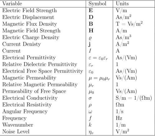
Table 2.1 shows the variables and constants used in this thesis.
2.1. ELECTRICAL CONDUCTION MECHANISMS 7
Table 2.1.: List of variables and constants. Bold characters represent vectors.
Variable Symbol Units
Electric Field Strength E V/m
Electric Displacement D As/m 2
Magnetic Flux Density B T = Vs/m 2
Magnetic Field Strength H A/m
Electric Charge Density ̺ As/m 3
Current Denisty j A/m 2
Current I A
Electrical Permittivity ε = ε 0 ε r As/(Vm) Relative Dielectric Permittivity ε r 1
Electrical Free Space Permittivity ε 0 As/(Vm) Magnetic Permeability µ = µ 0 µ r Vs/(Am) Relative Magnetic Permeability µ r 1
Permeability of Free Space µ 0 Vs/(Am)
Electrical Conductivity σ S/m = 1/(Ωm)
Electrical Resistivity ρ Ωm
Angular Frequency ω 1/s
Frequency f Hz
Wavenumber k 1/m
Noise Level η v V/m 2
2.1. Electrical Conduction Mechanisms
The physical property analysed in electromagnetic methods is the electrical conductivity σ or its inverse, the electrical resistivity ρ. The electrical conductivity is the capability of material to conduct electrical current, which can be influenced by three different mecha- nisms: Electronic, electrolytic and dielectric conduction (Telford et al., 1990). The effect of dielectric conduction can be neglected for the resistivities and the frequencies typically used in electromagnetics, and the relative electric permittivity ǫ r is not further consid- ered. Since most of the rocks are poor electronic conductors, the prominent mechanism is the one of electrolytic conduction. It is dependent on the porosity θ of the rocks, the arrangement and volume of its pores and the conductivity ρ w and saturation S of the fluid inside the pores and can be expressed with the empirical formula of Archie et al.
(1942) for the effective resistivity ρ e
ρ e = αθ −m S −n ρ w (2.1)
with n ≈ 2 and the constants 0.5 <= α <= 2.5 and 1.3 <= m <= 2.5. Note that Equa- tion 2.1, Archie’s law, only applies for rocks without clay or metallic minerals. When current is applied, chemical energy is stored in the material due to variations in the mo- bility of ions in the fluid throughout the rock structure (Telford et al., 1990). If clay particles are present, so called membrane polarisation effects are arising (Ward, 1990).
After the current is switched on, depending on the size of the rock pores, ions will accu-
mulate at one end of the rock fluid interface which decreases current flow. After switching
off the current, the ions will return to their original position, which will lead to a time
dependent decay of voltage. Another source of induced polarization is electrode polar- ization, which occurs if metallic material is present in the rocks and next to electrolytic conduction, metallic conduction appears. This will lead to an accumulation of ions in the electrolyte adjacent to the mineral particle. When the current is switched off, ions diffuse back to their original condition, which results in a transient decay of the residual voltage.
For example, graphite minerals can produce strong electronic polarization effects (Telford et al., 1990). Both, electronic and membrane polarization effects can be measured by the so called induced polarization (IP) method. Since in EM time (or frequency) dependent voltages are measured utilizing an alternating current signal, time and frequency depen- dent polarization effects can superimpose the induction response. In order to describe a frequency dependent resistivity ρ rock (ω), the Cole-Cole model (Cole and Cole, 1941) is utilized, where the induced polarization is expressed in terms of chargeability m, relax- ation time τ, the dispersion coefficient c and the time/frequency independent resistivity ρ 0 .
ρ(ω) = ρ 0
1 − m
1 − 1
1 + (iωτ ) c
(2.2) Since Graphite is present in the survey area, effects of induced polarization might super- impose the inductive response. Next to the frequency dependence, resistivity can depend on the direction of current flow. Then the resistivity is considered to be anisotropic, which typically occurs in stratified rocks such as slates or shales. Although anisotropy might occur in the area of study, in this thesis only isotropic resistivity is considered. Note that magnetic permeability µ r leads to an increased current induced into the ground (Telford et al., 1990), and therefore would affect the measured EM response. However, for most rocks, the magnetic permeability is around one. The basic principles of electromagnetic induction and measured field responses in time and frequency domain are given in the next chapter.
2.2. Maxwell Equations
The principal of electromagnetic induction is based on the Maxwell equations which de- scribe the behaviour of electromagnetic fields.
∇ × E = − ∂B
∂t (2.3)
∇ × H = ∂ D
∂t + j (2.4)
∇ · D = ̺ (2.5)
∇ · B = 0 (2.6)
where B is the magnetic induction, H is the magnetic field, D is the electric displace- ment, E is the electric field, j is the electric current density and ̺ is the electric charge density. Bold characters denote non-scalars. Additionally the quantities are linked by their constitutive relationships for a linear isotropic medium
B = µ o µ r H = µH (2.7)
2.2. MAXWELL EQUATIONS 9
D = ε o ε r E = εE (2.8)
j = σE (2.9)
where ε 0 is the permittivity of the free space, ε r the relative permittivity, µ 0 the perme- ability of the free space and µ r the relative permeability. Ohms law (2.9) describes the relationship between the total electric current density and the electrical conductivity σ for an isotropic conductor. For investigating the subsurface with CSEM, the relative per- meability µ r and permittivity ε r can be considered as scalar and frequency independent quantities and will be neglected, following that µ = µ 0 and ε = ε 0 . Furthermore, we assume that there are no free charges inside the earth, i.e. ̺ = 0. This leads to Equation (2.10)
∇ · j = 0 (2.10)
stating that there are no sources of current in the subsurface. Using these simplifications and Ohm’s law (2.9) as well as the constitutional relation (2.7) and (2.8), we can perform a transformation of the Maxwell Equations into the Telegrapher’s equations. If we multiply Equations (2.3) and (2.4) with ∇× , we obtain Equation (2.11).
∇ × ( ∇ × H) = − µ 0 σ ∂H
∂t − µ 0 ǫ ∂ 2 H
∂t 2 (2.11)
With the vector identity ∇ × ( ∇ × F) = ∇ ( ∇ · F) − ∆F and ∇ · F = 0, concluding
∇ × ( ∇ × F) = − ∆F we can derive the telegraphers equation.
∆ F = µ 0 σ ∂F
∂t + µ 0 ǫ ∂ 2 F
∂t 2 (2.12)
whereas F can either be E or H. The telegraphers equation can be transformed into frequency domain via Fourier transformation, rewriting the time derivative as ∂F/∂t = iω F. This leads to the Helmholtz equation
∆ F = iωµ 0 σ F − µ 0 ǫω 2 F (2.13)
In the period range used in CSEM applications σ ≫ ωε. Therefore, the second term of Equation 2.12 and 2.13 can be neglected and the equations utilizing the quasi static approximation (MT-Approximation) can be further simplified to
∆F = µ 0 σ ∂F
∂t (2.14)
∆F = iωµ 0 σF (2.15)
which is known as the diffusion equation in time and frequency domain.
2.2.1. Plane Wave Solution for a Uniform Conducting Halfspace
For plane electromagnetic waves the following equations applies
F = F 0 e i(ωt −kr) (2.16)
where F 0 is the amplitude, ω is the angular frequency and the wave number k = 1/λe r
is reciprocal to the wave length λ and points in the moving direction of the wave. Using
Equation (2.16), the spatial derivative can also be rewritten as ∆F = − k 2 F. Together with (2.15) this leads to
k = p
− iωµσ = 1 − i
√ 2
√ ωµ 0 σ (2.17)
With Equation (2.16) and (2.17) we can define the skin depth (2.18) that characterizes the penetration depth in which the amplitude of the electromagnetic wave is decayed to a 1/e of the initial surface value in case of a homogeneous subsurface.
δ F D = r 2
µ 0 ωσ or δ F D [km] ≈ 0.5 · p
ρ[Ωm] · T [s] (2.18)
2.2.2. Step Excitation Solution for a Uniform Conducting Halfspace
Ward and Hohmann (1988) give the impulse solution for EM Fields F at z = 0 in time domain as
F = F 0
√ µσz 2 √
πt 3 e −
µσz2
4t
(2.19)
Setting the derivative of Equation 2.19 to zero, the diffusion depth δ T D =
r 2t
µσ (2.20)
can be derived. It described the depth for a fixed t, at which the EM fields reach their maximum and is somewhat similar to the skin depth (Eq. 2.18) obtained in frequency domain. By forming the time derivative of the diffusion depth, one can obtain the velocity v T D , at which the maximum of the EM-fields is propagating (Ward and Hohmann, 1988).
v T D = 1
√ 2µσt (2.21)
2.3. HED Solution for a Uniform Conducting Halfspace
In order to get insights in the behaviour of the EM field components in time and fre-
quency domain for their corresponding data representations, we focus in the following
on the solution of a horizontal electrical dipole (HED) as utilized for LOTEM/CSEM
applications on the surface of a homogeneous halfspace. Equations and conclusion are
summarized from Kaufman and Keller (1983). The solution for both time and frequency
domain for a 1D layered or 2D case is somewhat more elaborate and the properties of
the different EM components are more in-transparent. For derivations of the EM field
solutions regarding a 1D layer case we refer to Kaufman and Keller (1983) or Ward and
Hohmann (1988). Weidelt (1986) approaches the solution over the separation of the EM
fields in TE and TM Mode. An analytical solution for a 1D case is not possible, since it
involves an iterative Bessel integral from a multiple number of layers, where the Hankel
transformation must be carried out numerically. For the problem formulation in 3D, refer
to Section 8.1.
2.3. HED SOLUTION FOR A UNIFORM CONDUCTING HALFSPACE 11
.
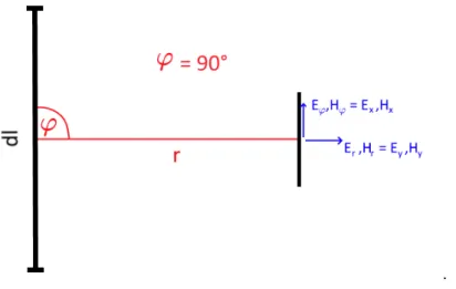
Figure 2.3: Definitions of field com- ponents utilized during the survey.
Having a broadside configuration, the EM field components reduce to E x , B y , and B z in case of a homo- geneous halfspace or a 1D layer case.
Therefore, subsequent formulas were simplified. The direction of r coin- cides with the y-direction, the direc- tion of x coincides with ϕ.
Field data is discussed as real and imaginary part in frequency domain and step on and step off transients in time domain in the subsequent sections. In order to get an un- derstanding for the behaviour of the collected field data, we differentiate between the solution for the named data representations in both domains. A HED excites always a combination of tangential electric (TE) and tangential magnetic (TM) fields. However, for the broadside configuration utilized during field measurements (Figure 2.3), the TE Mode dominates the response at the receiver locations. Therefore, the sensitivity towards resistive structures is low. Only E x , B y and B z components are 6 = 0. Next to the compo- nents of the TE-mode, during field measurements, B x was measured. B x deviating from 0 gives us therefore insights, if the conductivity distribution of the subsurface can be ap- proximated as 2D. However, being 0 for a homogeneous halfspace and our measurement configuration, it will not be discussed further in this section. Since we utilized the electric fields as validation for the frequency domain approach of the LOTEM dataset and studied different resolution behaviours in 1D and 2D for time and frequency domain, we focus on the electric field component in the following part, especially for the comparison between time and frequency domain. However, since a dense full component SQUID dataset was evaluated in frequency domain, the solution for the magnetic field is given for the sake of completeness. In the utilized 1D and 2D algorithms the forward solution is calculated in frequency domain and subsequently transformed into time domain via Fourier trans- formation. The following solutions are given for a point dipole. For an extended dipole, typically the solution of 10-20 single dipoles distributed along the transmitter wire is superimposed (cp. Section 8.2.1).
2.3.1. HED Solution in Frequency Domain
Under the assumptions given in Section 2.2, the EM Fields in frequency domain for a horizontal electrical dipole (HED) can be written as
E r = σIdl
2πσr 3 cos(ϕ)
1 + e kr (1 − kr)
(2.22) E ϕ = Idl
2πσr 3 sin(ϕ)
2 − e kr (1 − kr)
(2.23)
Note that the E z component due to boundary conditions equals 0 at the surface and is
therefore not further discussed.
p F D = r δ =
r σµω
2 r (2.24)
H r = − Idl
4πr 2 sin(ϕ)h r (p) (2.25) H ϕ = − Idl
4πr 2 cos(ϕ)h ϕ (p) (2.26) H z = Idl
4πr 2 sin(ϕ)h z (p) (2.27) The Equations 2.25-2.27 reflects the geometry dependency of the magnetic field. The factors h ϕ , h r , h z are dependent on the induction number p. For the full expression of the magnetic field components, refer to (Kaufman and Keller, 1983). Given the geometry depicted in Figure 2.3, for ϕ = 90 ◦ it follows E ϕ = E x , E r = E y = 0 and H ϕ = H x = 0 and H r = H y . Equations 2.22-2.23 and 2.25-2.27 simplify, if we considering low and high induction numbers separately.
2.3.2. Near Field Approximation FD
First we consider the near field zone of the transmitter, which is given for low induction numbers p F D ≪ 1, i.e. for small offsets and/or low frequencies. In order to differentiate the field solutions as real and imaginary parts, the term e kr is developed with a Taylor expansion, resulting in field solutions for real and imaginary part for the E x component.
ℜ E x ≈ − Idl 2πσr 3
1 + 1 3 √
2 (σµω) 3/2 r 3
(2.28)
ℑ E x ≈ Idl 2πσr 3
σµωr 2
2 − 1
3 √
2 (σµω) 3/2 r 3
(2.29) From Equation 2.28-2.29 we can conclude the following (after Kaufman and Keller (1983)):
• The first term of the real part can be thought as frequency independent galvanic term and depends on the resistivity of the medium. The second term is purely inductive, independent of the transmitter-receiver offset and is a function of σ and ω.
• The imaginary part is purely inductive. The first term is independent of conductivity but depends on the offset. It arises due to the change over time of the stationary magnetic field. The second term depends on the conductivity. Both terms are frequency dependent.
• For low frequencies (DC level) the imaginary part approaches zero. The real part
approaches the galvanic term, i.e. the stationary field which is proportional to the
resistivity.
2.3. HED SOLUTION FOR A UNIFORM CONDUCTING HALFSPACE 13 For the magnetic field component it follows for H z and H y
ℜ H z ≈ Idl 4πr 2
"
1 −
√ 2
15 (σµω) 3/2 r 3
#
(2.30)
ℑ H z ≈ Idl 4πr 2
"
1
4 σµωr 2 −
√ 2
15 (σµω) 3/2 r 3
#
(2.31)
ℜ H y ≈ Idl 4πr 2
1 − 3π 64 σµωr 2
(2.32)
ℑ H y ≈ Idl
4πr 2 (σµωr 2 ) 3
32 + 1 8 ln
√ σµωr 2
(2.33)
From Equation 2.30-2.33 we can conclude the following:
• Similar to the equations for the electric field, the real part of H z and H y consisting of the stationary magnetic field and a second inductive term, which is dependent on the frequency and conductivity. Note that the stationary part of the magnetic field is independent on the resistivity of the medium, unlike to the electric stationary field.
Note that this holds also for a horizontally layered case. Therefore, there is lower sensitivity of the magnetic field components towards the background resistivity.
• The frequency dependent second term of the real part for the H z component is more sensitive towards the conductivity than the respective terms in the E x and H y
components. Furthermore, the imaginary parts of the magnetic fields have a higher sensitivity to conductivity than the imaginary part of the E x component.
2.3.3. Far Field Approximation FD
In the next step, the behaviour for the far-field, i.e. large induction numbers (and therefore large values for k) is analysed, i.e. for large offsets and/or high frequencies. For the electric field holds
E x = − Idl
πσr 3 (2.34)
which follows directly from Equation 2.23, since k is a complex value. For the magnetic field, one can write
H y = − Idl
πkr 3 (2.35)
H z = 3Idl
2πk 2 r 4 . (2.36)
The derivation for H y and H z in terms of H r and H z can be found in Kaufman and Keller
(1983). We can summarize some conclusions:
• E x is real valued, frequency independent and coincides with the stationary field ( ∗ 2). Therefore, E x does not exhibit an inductive term for large induction numbers but is sensitive to the background resistivity.
• The magnetic field components are frequency dependent. Both are smaller than the stationary magnetic fields. The H z component decreases faster than H y with increasing offset to the source, however exhibits a higher sensitivity towards con- ductivity (1/k 2 vs. 1/k).
2.3.4. HED Solution in Time Domain
The EM solutions in frequency domain are connected to the solutions in TD by a unique Fourier transformation. In order to retrieve the time domain solution, the frequency domain response is transformed into time domain utilizing a sine or cosine transformation.
F off ( r , t) = − 2 π
Z ∞
0
ℑ (F(r, ω))
ω cos(ωt)dω (2.37)
F on (r, t) = 2 π
Z ∞
0
ℜ (F(r, ω))
ω sin(ωt)dω (2.38)
where r = (x, y, z) and F(r, t) the EM fields in space-time domain and F(r, ω) the EM fields in space-frequency domain. Equations 2.37-2.38 giving the transformations as im- plemented in the recently developed time domain solution (Haroon et al., 2018) of the 2D code MARE2DEM. Theoretically, the step off response can subsequently be calculated by subtracting the step on response from the DC response, following equation (Kaufman and Keller, 1983)
E of f = E DC − E on , (2.39)
where E DC is the stationary electric field corresponding to direct current conditions (ω = 0) and can be written for a homogeneous halfspace as
E DC = − Idl
2πσr 3 . (2.40)
This approach is implemented in the utilized time domain 1D algorithms EMUPLUS and MARTIN. Note that in order to solve the integrals given in 2.37-2.38, the solution must be calculated for a large number of frequencies in order to gain a stable forward solution (cp.
Section 8.2.10), which makes the solution in time domain computationally more expensive than in frequency domain. In the following, magnetic fields in time domain, H y and H z
(e.g. measured by SQUID magnetometer) or its time derivative dB y,z /dt (measured by
induction coils) refer to the corresponding component after switch off. We give the solution
for early and late time approximation for high and low induction numbers in analogy to
Section 2.3.1 for a homogeneous halfspace. For the general formulation for EM fields in
time domain on the surface of a conductor we refer to (Kaufman and Keller, 1983) or Ward
and Hohmann (1988). Similar to the frequency domain response for H ϕ (90 ◦ ) = H x = 0
and E r (90 ◦ ) = E y = 0. Solutions taken from Kaufman and Keller (1983) were simplified
2.3. HED SOLUTION FOR A UNIFORM CONDUCTING HALFSPACE 15 for an isotropic case in the following. Note, that throughout this thesis, the terms switch on and switch off response is utilized synonymously with the terms step on and step off response.
2.3.5. Near Field Approximation TD
The near field or late time approximation holds for small induction numbers p T D = δ r
T D
, i.e. for small offsets and/or late times.
H y = Idlσµ
64πt (2.41)
H z = Idlr 60
σµ πt
3/2
(2.42) In time domain typically the time derivative of the magnetic field is measured, when induction coils are utilized.
∂B y
∂t = − Idlσµ 2
64πt 2 (2.43)
∂B z
∂t (ϕ = 90 ◦ ) = − Idlσ 3/2 µ 5/2 r
40π 3/2 t 5/2 (2.44)
For electric fields we obtain:
E of f = − Idl 12π 3/2
r σµ 3
t 3 (2.45)
Therefore after current switch off, the electric fields approach zero for late times. Following Equation 2.39, electrical switch on and switch off response deviating only by the DC term 2.40 at any time t.
E on = − Idl
2πσr 3 + Idl 12π 3/2
r σµ 3
t 3 (2.46)
For large values of t, the electric field after switch on approaches the DC level. If one compares the field solution in time domain to the fields in frequency domain for small induction numbers, we notice, that the switch on solution for the near field approximation exhibits the same dependencies as the real part given in Equation 2.28. The switch off shows the same dependencies as the vortex term, i.e., the second term of the real part (cp. Eq. 2.28) and imaginary part (cp. Eq. 2.29) except for a constant factor. In the near field, the electric field component shows a dependency of p σ
t
3in time and √ σω 3 in frequency domain respectively. We conclude:
• For small induction numbers, the switch on electric field response is comparable to the real part of the electric field component in frequency domain
• The switch off response is comparable to the inductive term present in both, imag-
inary and real part. It is not superimposed by any additional term.
2.3.6. Far Field Approximation TD
The far field or early time approximation holds for large induction numbers p T D = δ r
T D