Research Collection
Educational Material
Introduction to Optimization
Author(s):
Fukuda, Komei Publication Date:
2020
Permanent Link:
https://doi.org/10.3929/ethz-b-000426221
Rights / License:
In Copyright - Non-Commercial Use Permitted
This page was generated automatically upon download from the ETH Zurich Research Collection. For more information please consult the Terms of use.
ETH Library
Introduction to Optimization
Komei Fukuda
Department of Mathematics, and Institute of Theoretical Computer Science
ETH Zurich, Switzerland fukuda@math.ethz.ch
ETH Book Project, 2018-07-30;Rev 2020-07-14
2
Komei Fukuda
Department of Mathematics, and
Institute of Theoretical Computer Science ETH Zurich, Switzerland
fukuda@math.ethz.ch
Copyright©˙2020 Komei Fukuda ISBN ˙978-3-906916-73-6
All rights reserved. This work may not be translated in whole or in part without the written permission of the author. The work can be copied in whole, meaning that the copy must be complete and hence it must include this copyright statement. The commercial sale of the work or any derivative product by the third party is strictly prohibited.
The moral right of the author has been asserted.
Contents
Preface i
1 Introduction to Linear Programming 1
1.1 Importance of Linear Programming . . . . 1
1.2 Examples . . . . 2
1.3 Linear Programming Problems . . . . 4
1.4 Solving an LP: What does it mean? . . . . 6
1.5 History of Linear Programming . . . . 7
1.6 Exercises . . . . 9
2 LP Basics I 11 2.1 Recognition of Optimality . . . . 11
2.2 Dual Problem . . . . 13
2.3 Recognition of Infeasibility . . . . 15
2.4 Recognition of Unboundedness . . . . 16
2.5 Dual LP in Various Forms . . . . 18
2.6 Exercises . . . . 19
3 LP Basics II 21 3.1 Interpretation of Dual LP . . . . 21
3.2 Exercise (Pre-sensitivity Analysis) . . . . 23
3.3 Sensitivity Analysis . . . . 24
3.4 Exercises . . . . 26
4 CONTENTS
4 LP Algorithms 29
4.1 Matrix Notations . . . . 30
4.2 LP in Dictionary Form . . . . 31
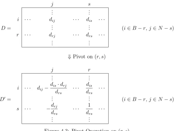
4.3 Pivot Operation . . . . 38
4.4 Pivot Algorithms and Constructive Proofs . . . . 41
4.4.1 The Criss-Cross Method and a Proof of Strong Duality . . . . 41
4.4.2 Feasibility and Farkas’ Lemma . . . . 46
4.4.3 The Simplex Method . . . . 48
4.5 Examples of Pivot Sequences . . . . 52
4.5.1 An example of cycling by the simplex method . . . . 52
4.5.2 Simplex Method (Phase II) applied to Chateau Maxim problem . . . 53
4.5.3 Criss-Cross method applied to Chateau Maxim problem . . . . 54
4.5.4 Criss-Cross method applied to a cycling example . . . . 55
4.5.5 Simplex method with Bland’s rule applied to a cycling example . . . 56
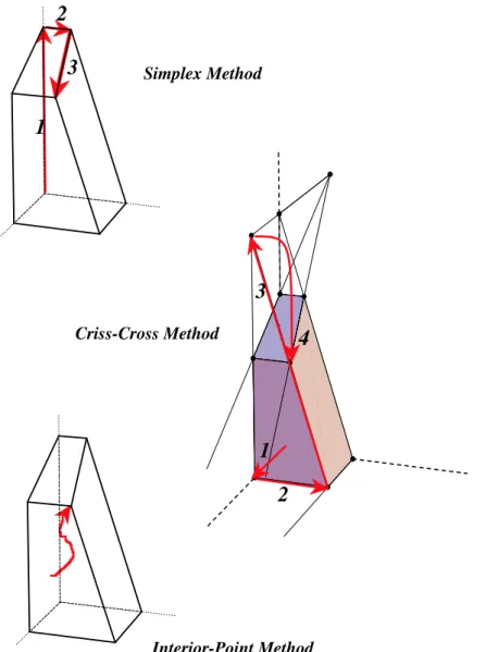
4.6 Visual Description of Pivot Algorithms . . . . 57
4.6.1 Simplex Method . . . . 57
4.6.2 Criss-Cross Method . . . . 58
4.7 Exercises . . . . 58
5 LP Advanced Topics 61 5.1 Implementing Pivot Operations . . . . 61
5.2 Computing Sensitivity . . . . 63
5.3 Dualization of Pivot Algorithms . . . . 64
5.4 Pivot Rules for the Simplex Method . . . . 65
5.5 Geometry of Pivots . . . . 67
5.5.1 Geometric Observations of the Simplex Method . . . . 67
5.5.2 Three Paradigms of LP Algorithms . . . . 70
5.5.3 Formal Discussions . . . . 71
5.6 Exercises . . . . 75
6 Combinatorial Optimization and Complexity 77
CONTENTS 5
6.1 Examples . . . . 78
6.2 Efficiency of Computation . . . . 81
6.2.1 Evaluating the Hardness of a Problem . . . . 82
6.2.2 A Little History . . . . 85
6.3 Basic Graph Definitions . . . . 85
6.3.1 Graphs and Digraphs . . . . 85
6.4 Exercises . . . . 90
7 Polynomially Solvable Problems 93 7.1 Minimum-weight Spanning Tree Problem . . . . 93
7.2 Bipartite Perfect Matching Problem . . . . 94
7.3 Assignment Problem . . . . 96
7.4 Optimal Matching Problem . . . . 99
7.5 Maximum Flow Problem . . . 101
7.6 Minimum Cost Flow Problem . . . 103
7.6.1 Exercise (Toy Network Flow Problems) . . . 104
7.7 Exercises . . . 105
8 Exhaustive Search and Branch-and-Bound Algorithms 107 8.1 Branch-and-Bound Technique . . . 107
8.2 Exercises . . . 113
9 Cutting-Stock Problem and Column Generation 115 9.1 Cutting-Stock Problem . . . 115
9.2 The Simplex Method Review . . . 117
9.3 Column Generation Technique . . . 118
9.4 Exercises . . . 119
10 Approximation Algorithms 121 10.1 Set Cover Problem . . . 121
10.2 Greedy Algorithm . . . 123
10.3 Primal-Dual Algorithm . . . 124
6 CONTENTS
10.4 LP-Rounding . . . 126
11 Interior-Point Methods for Linear Programming 129 11.1 Notions . . . 130
11.2 Newton’s Method . . . 132
11.3 Primal-Dual interior-Point Methods . . . 133
11.3.1 Newton’s Method Directly Applied to F . . . 135
11.3.2 The Central Path . . . 136
11.3.3 Polynomial Complexity . . . 137
11.3.4 How Important is Polynomial Complexity in Practice? . . . 139 A Some Useful Links and Software Sites on Optimization 141
Preface
Here, we introduce some basic notions and results in optimization in plain language so that the reader can foresee the materials of the book without the strict mathematical formalism.
In particular, this is for the reader to understand the key differences of the three main themes of optimization, linear, combinatorial and nonlinear optimization. Note that because of intuitive and bird’s-eye nature of the overview, we may not give proper mathematical definitions of some terms used.
Linearity and Nonlinearity
Let’s look at the following photo, an image capturing the landscape of the Swiss alpine region of the Matterhorn and the new Monte Rosa Hut1 nearby.
It is not difficult to notice a stark difference in geometric shape of the natural landscape and the manmade hut.
First of all, the shape of the hut is essentially a convex polytope, like many familiar shapes with a simple mathematical description such as a cube , a tetrahedron or a dodecahedron.
1The Monte Rosa Hut was designed by the architect Andrea Deplazes of ETH Zurich and inaugurated in 2009. The photo is taken from http://www.deplazes.arch.ethz.ch/article?id=5ab8cede4258bdoc2013539015.
The permission to use the photo was granted by the architect to whom the author is grateful.
ii Preface One simple fact about these “linear” and “convex” objects suggests a nice property: a point is a highest point if it is a locally highest point. Moreover, there is always a corner point (vertex) of the hut that is a highest point. This means that if one wish to find a highest point of the hut, you just have to find a vertex which has no higher vertex in its neighborhood. It naturally suggests an algorithm that moves (pivots) from any vertex of the hut, moves along the edges incident to it as long as it moves to a higher vertex. This algorithm works in any dimension as this is one of the most fundamental results in what we calllinear programming, the subject of Chapters 1 – 5. The algorithm is known as the simplex algorithm, invented by George Dantzig in 1947 and will be presented in Chapter 4. Its practical efficiency is widely recognized and one can arguably say that the importance of optimization relies on this unquestionable efficiency. In fact, in order to solve harder optimization problems, such as nonlinear programming and combinatorial optimization, we often rely on the fact that linear programming can be solved efficiently.
Here is a natural question, is the Matterhorn peak the highest peak in the neighborhood, say within the radius of 50 km? We are talking about the nature of the underlying math- ematical question but not about the geographic knowledge of our planet. For this kind of mathematical question, one needs to assume that the height (altitude) of a given location p = (x, y) is given as a function f(p). In order to make the question even more concrete, one may assume that the function is a piece-wise linear approximation, just like a computer graphics technique of representing a nonlinear surface by a surface of triangular patches. In such a model, it is easy to find a local peak vertex (a corner of a triangle patch) that has no higher neighbor vertex, using a simplex-method like method. The hard part is to decide whether a given local peak is a global peak. This naturally leads to an obvious method of enumerating all local peaks and exhibiting the highest peak(s). Is this the only way to find a highest peak? Such a method needs to evaluatef(p) at all vertices pin the region. Unless other property is known about the function, one cannot expect anything better, because one can fool any “faster” algorithm by modifying the function where the algorithm does not evaluate. This shows the inherent hardness ofnonlinear optimization that becomes extraor- dinarily harder (or practically impossible) when each point p lies in a higher dimensional space.
Alternatively, we may assume instead that the height function is given by a smooth continuous approximation. Such a function is differentiable (i.e. has a derivative). Then one can apply different type of algorithms, such as the steepest ascent algorithm which moves from any point to search for the highest point along the direction of a steepest derivative.
But, under the assumption of smoothness and continuity, a local peak is merely a local peak and there is no good characterization of a global peak that avoids the comparisons with all local peaks. The most important special case of nonlinear optimization is convex where a local peak is a global peak. This leads to the important theory of convex programming.
By the way, the reader may wish to know the answer to the geographic question. It might be surprising that the peak of the famous Matterhorn is not the highest peak in the area. It is 4478m, while the peak of the Monte Rosa (hidden in the photo and far left above the hut at height 2795m) is 4634m and the highest in Switzerland.
In this book, we will not discuss how one can deal with all sorts of difficulties ofnonlinear optimization. This is a diverse subject that should be treated separately, and it is a natural
iii continuation of the basic optimization the book addresses.
Nevertheless, we shall discuss one important class of algorithms in convex programming, known as interior-point methods. Such technique applied to a linear programming is theo- retically superior to any methods based on pivoting operation, described above. This will be discussed in Chapter 11.
Combinatorial Nature of Human Life
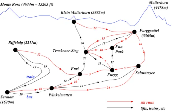
A few hundreds meters below the Monte Rosa Hut, a famous “paradise” for skiers and mountain lovers spreads wide and tall, known as the Zermatt Ski Resort. The whole area is extremely diverse and it accommodates a countless number of ski runs (slopes). Then, there are lots of transportation means such as ski lifts, ropeways and even trains. Figure 0.1 illustrates a much simplified version of the resort.
Zermatt (1620m)
Riffelalp (2211m)
Trockener-Steg
Winkelmatten
Schwarzsee Klein Matterhorn (3885m)
Matterhorn (4478m)
Furi
Furgg Fun Park
Furggsattel (3365m)
train
bus
Monte Rosa (4634m = 15203 ft)
ski runs lifts, trains, etc
19 19
12
20
20 18
12
10
15
11 12
22
15 9
10
16
24 10
10
5
5 7
Figure 0.1: Zermatt Ski Resort (much simplfied)
Imagine that the real resort is actually 5 times larger. For anyone visiting the resort for skiing, it is quite a challenge to make a good skiing plan. This naturally leads to a general question of finding an optimal skiing plan.
To make the meaning of optimality precise, Figure 0.1 contains a number on each run which is the time (in minutes) to complete the run (for a hypothetical skier). and similarly the time of a ride for the transportation means. Of course, these numbers vary depending on weather, snow condition, crowdedness, etc. For simplicity, let’s assume that these numbers are correct.
iv Preface Now, we can set a simple optimization problem that any skier unfamiliar with the ski resort wishes to solve:
(i) what is the shortest time to do all ski runs, starting and ending at the Zermatt town?
An even simpler question is:
(ii) can one do all ski runs in less than four hours?
The first problem (i) is a typical optimization problem, that is, to minimize (or maximize) some objective measure under a set of constraints. The second problem (ii) is different in that the answer is either yes or no. A problem of this type is known as adecision problem.
The optimization problem (i) is of combinatorial in nature, it’sfeasible solution (sched- ule) is a sequence of ski runs, lifts, ropeways and train in a way that one covers all ski runs.
A feasible solution isoptimal if the total time is smallest among all feasible solutions. Unlike in linear and nonlinear optimization, the set of all feasible solutions is a discrete set where there is no feasible solution in between two solutions. In the hight maximization problem, any location within the given region (say a disk of 50km radius) is feasible and a candi- date of optimal solution. That’s a reason why we will call the problem (i) a combinatorial optimization problem.
Associated with any given optimization problem like (i), the simpler problem (ii) is known as the associateddecision problem, namely asking
(ii’) does there exist a feasible solution whose objective value is less than k?
where k is any given constant. In the case of optimization problems of maximization, one replaces “less” with “more.” The key importance of this question is to determine whether a given feasible solution with objective value k is optimal or not.
If the answer to (ii’) is yes, a certificate is a feasible solution whose objective value is less thank. A certificate is any information with which one can verify the correctness of the answer. A certificate is good if the time for verification is quick, more precisely, the time is bounded by a polynomial function of the input size. In case of (ii), it is just a feasible ski plan whose total time is less than 4 hours, and it is very easy to check the given plan covers all ski slopes and its total time is less than 4. When a good certificate exists for any “yes”
instances of an optimization problem, the problem is said to belong to the class NP. The decision problem of the ski runs optimization type is in the class NP.
If the answer to (ii’) is no, what could be a good certificate? In the specific case of the ski runs (ii), when there is no feasible plan to cover all ski slopes in less than 4 hours, what would be a good certificate? Typically, to prove the nonexistence of a feasible solution (with an additional property) is not easy, as one might easily guess. When a good certificate exists for any “no” instances of an optimization problem, the problem is said to belong to the classco-NP. These concepts of NP and co-NP are central themes of the computational com- plexity theory, which will be discussed in Chapter 6. Various spacial cases of combinatorial optimization problems will be discussed in Chapter 7 through Chapter 10.
v It is not obvious that the decision problem of the ski runs optimization type is also in co-NP, thus in both NP and co-NP. These facts help us to design a very efficient algorithm for the ski runs optimization problem, to be discussed in Chapter 7. The ski runs problem may not sound very important in practice. However, this type of visiting certain fixed parts of a network as quickly as possible appears in many practical settings, such as the postman’s delivery of mails and the delivery of lunch boxes to the clients, and these can be solved by essentially the same efficient algorithm.
Unlike the problems in NP ∩ co-NP, there are problems that appear not to belong to this class. The hardest problems in NP have the property that if anyone of them is proven to be in co-NP then every one of them is in co-NP. These hardest problems are called NP- complete. An NP-complete problem is such that we don’t know any easy way to prove that there is no better solution than a given feasible solution. The situation is similar to the general nonlinear optimization like the highest peak problem where there is no good way to say a given local peak is a global peak. There are many different approaches to solve NP-complete problems, such as the branch-and-bound technique (Chapter 8), the column- generation algorithm (Chapter 9) and approximation algorithms (Chapter 10).
The Structure of the Book
As explained in the previous section, the book addresses mainly two themes, (1) linear optimization and (2) combinatorial optimization. We also present (3) a limited account of nonlinear optimization techniques. Learning the contents of (1) is essential for understanding both (2) and (3), while the subjects (2) and (3) are independent and can be read separately.
Below we summarize the key contents of the book, and how they can be used in class- rooms.
(1) Linear Programming: The basic theory of linear programming is given with a min- imal set of mathematical terminologies in Chapters 1, 2 and 3. These chapters cover the most important theoretical results without proofs, and can be used to teach un- dergraduate or graduate students in nonscientific majors, with the aide of computer software.
Two algorithms for linear programming are presented in Chapters 4 and 5 with rigorous mathematical proofs of finite termination. These algorithms are the criss-cross method and the simplex method. To follow these chapters, one needs a good training in linear algebra and proof techniques.
(2) Combinatorial Optimization: The computational complexity theory is introduced in Chapter 6, together with many problems in combinatorial optimization. The notions like the class P, NP, co-NP and NP-complete will be discussed there. This chapter and the LP theory chapters (1) are the prerequisites to continue on Chapters 7 – 10.
Chapter 7 is devoted to the polynomially solvable cases, namely the problems in class P. The assignment problem, the minimum-weight spanning tree (MST) problem and the general matching problem are discussed among others. This chapter is extremely important to understand the power of complexity theory.
vi Preface Chapters 8 – 10 present different approaches to solve NP-complete or possibly harder problems. Chapter 8 is devoted to the branch-and-bound algorithm which is applicable to a large class of hard problems. Chapter 9 discusses the column generation algorithm that can be used to solve practically a large-scale LP where the input is not explicitly given. This chapter uses the technique given in Chapter 8.
Chapter 10 presents various techniques to find an approximate solution to hard opti- mization problems. This chapter does not depend on Chapters 8 and 9.
(3) Nonlinear Programming: Our objective here is to study modern nonlinear program- ming techniques to design a polynomial-time algorithm for linear programming. Chap- ter 11 presents key components of the so-called path-following primal-dual algorithm applied to linear programming. This chapter does not depend on Chapters 7 – 10.
Three Main Themes in Mathematical Formulation
Let us give the three optimization themes in mathematical form, using the standard matrix notation. Below A is a given rational matrix of size m× n where m and n are natural numbers, b is a given column (rational) vector of size m, c is a given (rational) column vector of size n.
1. Linear Programming or Linear Optimization (LP) maximize cTx (x∈Rn) subject to Ax ≤ b
x ≥ 0.
Solvable by highly efficient algorithms. Practically no size limit. The duality theorem plays a central role. Chapters 1–3 gives the basic theory of LP without hard proof, while Chapters 4 and 5 presents mathematically correct description of two algorithms, the criss-cross method and the simplex method with rigorous proofs and geometric interpretations.
2. Combinatorial Optimization
maximize cTx
subject to x ∈ Ω.
Here Ω is a “discrete” set, e.g.
Ω = {x∈Rn:Ax≤b, xj = 0 or 1 for allj}, or
Ω ={x∈Rn:x represents a certain set of edges in G},
where G is a given graph and “certain” must be defined properly, such as a path connecting two fixed vertices inG.
vii The first example above is the case of 0/1integer linear programming while the second one is a typical case of graph or network optimization.
The combinatorial optimization includes both easy and hard problems, namely, P (polynomially solvable) and NP-complete (or NP-hard). The 0/1 integer linear pro- gramming is known to be NP-complete, a key result in the theory of integer linear programming which is beyond the scope of the present book. We shall learn how to recognize the hardness of various graph/network optimization problems and how to select appropriate techniques in Chapters 7 – 10.
3. Nonlinear Programming or Nonlinear Optimization (NLP) maximize f(x)
subject to gi(x)≤ 0 for i= 1, . . . , m,
where f(x) and gi(x) are given real-valued functions: Rn→R.
Convexity plays an important role. Interior-point algorithms solve convex and well- formulated NLP efficiently, including LP. We concentrate our attention to polynomial interior-point algorithms applied to LP in Chapter 11.
How To Use This Book
The ideal targets of this book are those students who took a good rigorous course in linear algebra and are familiar with basic proof techniques. This group, we call the group I, can benefit most from this book. Nevertheless, other groups should be able to use this book, but to get the maximum profit out of the book, it is important for the instructor to know what to teach and what to skip. Let us call the group II those who studied linear algebra for mainly practical purposes without rigorous proofs. The third group group III consists of those who have not taken any linear algebra course, typically those in nonscientific disciplines. We give concrete advises for each of these groups.
[Group I ] Follow the book in the order of chapters. One should be able to teach all the materials in one semester, but if the time becomes tight, the instructor may either skip one of Chapters 10 and 11, or give brief presentation of them. Unlike the other chapters, Chapter 11 relies on some notions from analysis or calculus, and it is meant to give students the flavor of nonlinear optimization so that the students can decide whether to take a course on this advanced subject later. Therefore, the instruction may exclude Chapter 11 from the final examination, unless a rigourous analysis/calculus course is added to the prerequisites.
[Group II ] Follow the book in the order of chapters. Some proofs might be skipped but try to teach how to prove simple statements like the weak duality theorem, Theorem 2.1.
For harder theorems, like the strong duality theorem, Theorem 2.2, the instructor can still give an overview of the proof. Make good use of available LP codes (open source or commercial), and give exercises that require the use of computer codes. Chapters
viii Preface 10 and 11 can be exempted from the final examination, although the instructor might want to summarise their contents to the students without proofs.
[Group III ] Use the first three chapters (LP introduction and basics) only. These chapters are written in such a way that the key results in linear programming can be understood without any knowledge of linear algebra except for matrix and vector notations. Make good use of an available LP code (open source or commercial) so that the students learn the basic LP concepts by solving simple LP instances. It is important that the students learn how to read both optimal and dual optimal solutions correctly, and to be able to explain the meaning of the sensitivity analysis.
Aknowledgements
I sincerely thank my mentors of mathematics Jack Edmonds, Tomoharu Sekine, Hisakazu Nishino, Masakazu Kojima for their great passion for beautiful mathematics. I am most grateful to Thomas Liebling, Hans-Jakob L¨uthi, Emo Welzl, Bernd G¨artner, David Avis, Tam´as Terlaky, Lukas Finschi and David Adjiashvili for friendship and mathematical collaborations. There are so many others who deserve to be mentioned, in particular many teaching assistants at ETH Zurich for the courses “Optimization Techniques” and “Introduction to Optimization” that I taught. Finally, my most af- fectionate thanks go to my wife. Without her support, this work would not have existed.
Chapter 1
Introduction to Linear Programming
1.1 Importance of Linear Programming
Linear programming (abbreviated by LP), also known as linear optimization, is the most fundamental subject of optimization whose importance in the entire subject of optimization cannot be overstated. It is the subject that influences practically every other subjects both theoretically and practically. In the theoretical frontier, the LP theory consists of duality and efficient algorithms is in ideal form of optimization theory. On the other hand, practitioners in optimization are relying on implementations of LP algorithms that are extremely fast even for very large scale problems. The availability of both free and commercial codes helps a great deal in generating practical applications of LP algorithms to wide ranges of situations in industries, engineering, sciences and even policy making.
Here is a quick summary of the importance of LP techniques.
Many applications Optimum allocation of resources, transportation problems,, maximum and minimum-cost flows, work force planning, scheduling, etc.
Large-scale problems solvable Simplex method (Dantzig,1947), Interior-point methods (Karmarkar et al. 1984 –), Combinatorial methods (Bland et al. 1977 –).
One can solve LP’s with a large number (up to millions) of variables and constraints, and there are many reliable LP codes available:
• Commercial codes: CPLEX, IMSL, LINDO, MINOS, MPSX, XPRESS-MP, etc.
• Free software packages: LPsolve, SoPlex, glpk, etc.
Helping to solve much harder problems: LP solvers are used to solve much harder problems in concert with additional optimization techniques such as the branch-and- bound (Chapter 8), the column generation (Chapter 9) and approximation algorithms (Chapter 10). These harder problems include hard combinatorial optimization prob- lems and general integer linear programming problems.
Beautiful theory behind it! It says everything.
2 Introduction to Linear Programming
1.2 Examples
Let’s look at a simple setting of linear programming where we have a limited supply of re- sources to produce multiple products with different profits. Such production optimization is widely known as the optimum allocation of resources which appear in numerous applications.
Example 1.1. Optimum allocation of resources
Chateau Maxim produces three different types of wines, Red, Rose and White, using three different types of grapes planted in its own vineyard. The amount of each grape necessary to produce a unit amount of each wine, the daily production of each grape, and the profit of selling a unit of each wine is given below. How much of each wines should one produce to maximize the profit? We assume that all wines produced can be sold.
wines
Red White Rose
grapes supply
Pinot Noir 2 0 0 4
Gamay 1 0 2 8
Chardonnay 0 3 1 6
(ton/unit) (ton/day)
3 4 2
profit (K $/unit)
Here are a sequence of straightforward approaches for the best production:
• Why not to produce the most profitable wine as much as possible?
Limit of 2 units of white.
• The remaining resources allows 2 units of red. So, we can produce 2 units of red, 2 units of white. This yields the profit of 14 K dollars.
• By reducing 1 unit of white, one can produce 2 units of red, 1 unit of white, 3 units of rose.
This generates the profit of 16 K dollars.
Some natural questions arise, and how do you answer them?
Question 1 Is the second plan the best production? How can one prove it?
Question 2 Maybe we should sell the resources to wine producers? And at what price?
Question 3 How does the change in profitability affect the decision? What about the change in the supply quantities?
In order to answer these questions, formulating the problem of profit maximization math- ematically is crucial.
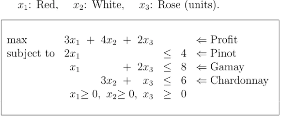
1.2 Examples 3 Vineyard’s Primal LP (Optimize Production)
Let us denote byx1 the unit of red wine to be produced, similarly x2 for white wine and x3 for rose wine. With these variables, the total profit is easily written as a linear function 3x1 + 4x2 + 2x3, and the constraints on these variables can be written by a set of linear inequalities as follows:
max 3x1 + 4x2 + 2x3 ⇐Profit
subject to 2x1 ≤ 4 ⇐Pinot
x1 + 2x3 ≤ 8 ⇐Gamay
3x2 + x3 ≤ 6 ⇐Chardonnay x1≥0, x2≥0, x3 ≥ 0 ⇐Production
Remark 1.1. When any of the variable(s) above is restricted to take only integer values 0, 1, 2, . . ., the resulting problem is called an integer linear program (ILP) orinteger program (IP) and much harder to solve in general because it belongs to the class NP-complete, the notion discussed in Chapter 6. There are some exceptions, such as the assignment problem and the maximum flow problem, that can be solved very efficiently.
Remark 1.2. It is uncommon to mix red and white grapes to produce a rose wine. A typical way is by using only red grapes and removing skins at an early fermentation stage. Thus, our wine production problem (Example 1.1) does not reflect the usual practice. Nevertheless, mixing different types of grapes, in particular for red wines, is extremely common in France, Italy and Switzerland.
Example 1.2. Optimum allocation of jobs
Maxim Watch Co. has P workers who are assigned to carry out Q tasks. Suppose the worker i can accomplish mij times the work load of task j in one hour (mij >0). Also it is required that the total time for the worker i cannot exceed Ci hours. How can one allocate the tasks to the workers in order to minimize the total amount of working time?
Mathematical Modeling
Letxij be the time assigned to worker i for taskj.
min X
i,j
xij subject to
Q
X
j=1
xij ≤Ci (i= 1, . . . P),
P
X
i=1
mijxij = 1 (j = 1, . . . , Q),
xij ≥0 (i= 1, . . . P;j = 1, . . . , Q).
4 Introduction to Linear Programming
1.3 Linear Programming Problems
A linear function f of n real variables x1, x2, . . ., xn is defined as f(x1, x2,· · · , xn) =c1x1+c2x2+· · ·+cnxn wherec1, c2,· · ·, cn are given real constants.
A linear equality over real variablesx1, x2, . . .,xn is f(x1, x2,· · · , xn) =b wheref is a linear function and b is a given constrant.
A linear inequality over real variables x1,x2, . . ., xn is defined as either f(x1, x2,· · · , xn)≥b or
f(x1, x2,· · · , xn)≤b whereb is a given constant.
A linear constraint means either a linear equality or an inequality.
Alinear programming problem or anLP is defined as a problem to maximize or minimize a linear function over a finite set of linear constraints:
max c1x1+c2x2+· · ·+cnxn
subject to ai1x1+ai2x2+· · ·+ainxn =bi (i= 1,· · · , k) ai1x1+ai2x2+· · ·+ainxn ≤bi (i=k+ 1,· · · , k0) ai1x1+ai2x2+· · ·+ainxn ≥bi (i=k0+ 1,· · ·, m).
Here, c1x1+c2x2+· · ·+cnxn is called theobjective function.
1.3 Linear Programming Problems 5 Quiz Decide for each of the following problems whether it is an LP or not.
1.
max 2x + 4y
subject to x − 3y = 5 y ≤0 2.
max 2x + 4y
subject to x − 3y = 5 x ≥0 or y ≤0 3.
max x + y + z
subject to x + 3y − 3z <5
x − 5y ≥3
4.
min x2 + 4y2 + 4xy
subject to x + 2y ≤4
x − 5y ≥3
x≥0, y ≥0 5.
min x1 + 2x2 − x3 s. t. x1 ≥0 x2 ≥0
x1 + 4x2 ≤4
x2 + x3 ≤4 x1, x2, x3 are integers.
6.
min 2x1 − x2 − 3x3
s. t. x1 + 4x2 ≤4
x2 + x3 ≤4 x1 ≥0 x2 ≥0
x1 is integer.
7.
min x1 + 2x2 − x3
s. t. x1 + 4x2 + x3 ≤ 4 3x1 x2 + x3 ≤ 4 x1, x2, x3 are either 0 or 1.
6 Introduction to Linear Programming
1.4 Solving an LP: What does it mean?
Key words
optimal, unbounded, infeasible
Let us recall the optimal production problem of Chateau Maxim:
x1: Red, x2: White, x3: Rose (units).
max 3x1 + 4x2 + 2x3 ⇐Profit
subject to 2x1 ≤ 4 ⇐Pinot
x1 + 2x3 ≤ 8 ⇐Gamay
3x2 + x3 ≤ 6 ⇐Chardonnay x1≥0, x2≥0, x3 ≥ 0
• A feasible solution is a vector that satisfies all constraints:
(x1, x2, x3) = (0,0,0) yes (x1, x2, x3) = (1,1,1) yes (x1, x2, x3) = (2,1,3) yes (x1, x2, x3) = (3,0,0) no (x1, x2, x3) = (2,−1,0) no
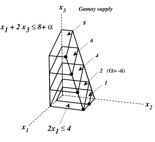
• A feasible region is defined as the set Ω of all feasible solutions x = (x1, x2, x3)T. Figure 1.1 shows this region. Geometrically the feasible region is a convex polyhedron.
x3
x1
x2
2 x1≤ 4 x1 + 2 x
3≤ 8
3 x2 + x 3≤ 6
Figure 1.1: Feasible Region Ω
1.5 History of Linear Programming 7
• An optimal solution is defined as a feasible solution that optimizes (maximizes or minimizes) the objective function among all the feasible solutions.
• LP may not admit an optimal solution. There are two such cases:
(1) Infeasible case
max x1 + 5x2
subject to x1 + x2 ≥ 6 ←conflicting
−x1 − x2 ≥ −4 ←constraints This LP has no feasible solution. =⇒It is said to be infeasible.
(2) Unbounded case
max 2x1 − x2
subject to −x1 + x2 ≤ 6
−x1 − 3x2 ≤ −4
The objective function is not bounded (above for maximization, below for minimiza- tion) in the feasible region. More formally it means that for any real numberk there ex- ists a feasible solution whose objective value is better (larger for maximization, smaller for minimization) than k.
=⇒ An LP is said to beunbounded.
• The first important theorem about LP is what we call the fundamental theorem of linear programming :
Theorem 1.3. Every LP satisfies exactly one of the three conditions:
(1) it is infeasible;
(2) it is unbounded;
(3) it has an optimal solution.
• Solving an LP means
Problem 1.1 (Solving an LP). Given an instance of LP, derive the conclusion 1, 2 or 3, and exhibit its certificate.
For example, the simplex method is a method solving an LP. A certificate is an extra information with which one can prove the correctness of the conclusion easily. We shall see certificates for 1, 2 and 3 in Chapter 2.
1.5 History of Linear Programming
The history of linear programming is diverse and still expanding with new results and new applications.
8 Introduction to Linear Programming The birth of linear programming is widely accepted as 1947 when George B. Dantzig invented a highly effective algorithm for linear programming, known as the simplex method.
Dantzig also coined the term “linear programming” to represent the fundamental problem of maximizing/minimizing a linear function over a finite set of linear inequality/equality con- straints. The year 1947 is also important as the birth year of the linear programming duality theory by John von Neumann. This theory together with the simplex method constitutes the initial foundation of linear programming.
Below is a simple diagram of critical events that lead to the subject of linear programming and mathematical optimization, which has become immensely important in our modern so- ciety demanding all sorts of optimization in intelligent machines and systems. The diagram below is an excerpt from Dantzig’s signature book [9][Section 2-1] with some recently discov- ered results. The reader is strongly encouraged to read the book, especially for the history of linear programming, to learn from the great mathematician who made the foundation of linear programming.
Military Economy/Industry Linear Programming Mathematics
Military 20th Century
Input-Output Model Leontief (1936)
Inequality Theory Fourier (1923) Gordan (1873) Farkas (1902) Motzkin (1936) Economic Model
Kantrovich (1939)
Game Theory von Neumann &
Morgenstern (1944) Linear Programming
(1947)
Simplex Method Danzig (1947) Economic Model
Koopmans (1948)
Duality Theory von Neumann (1947) Nobel Prize
Leontief (1973) Koopmans and Kantorovich (1975)
Combinatorial Algo.
Bland etc. (1977 ) Polynomial Algo.
Khachiyan (1979) Opt. resourse alloc.
New Polynomial Algo.
Karmarkar (1984)
In the field of mathematics, “linear programming” was studied before its name was de- fined. Theory of linear inequalities was a classical subject that were studied much before 1947 by Fourier, Farkas, Motzkin, and others. It turns out that solving a linear inequality system is essentially equivalent to solving a linear program, by the LP duality of von Neu- mann. A method known as the Fourier-Motzkin algorithm in fact can be used to solve an LP but it is far inferior to the simplex method.
In the economic and industrial front, many research results closely related to linear programming appeared earlier than 1947. The Leontief Input-Output Model, proposed in 1930’s, is a global model of economic activities that analyses how the productions of dif-
1.6 Exercises 9 ferent sectors interlinked within a system (e.g. a country) can be sufficient to produce the demands of the system. It is formulated as a linear system of equations with production variables that are nonnegative. Leonid Kantorovich formulated a real-life problem in the plywood industry in the soviet union as a linear programming as early as 1938 when the term “linear programming” was unknown. He devised a solution method using ideas from functional analysis. His work was unknown to the western world until mid 1940’s. Another mathematician who contributed greatly in formulating economic models as linear program- ming is Tjalling C. Koopmans. In 1942, he proposed an economic model of transportation networks, and studied optimal routing. Later, he communicated with Dantzig and others to develop a versatile modelling of optimal allocation of resources in late 1940’s.
In the algorithmic development front, a new type of algorithms was invented by Robert Bland in 1977. These are called combinatorial algorithms for linear programming, because the finiteness of these algorithms are not based on the real numbers but the strict improve- ment on certain combinatorial structures at each algorithmic steps. We will use one of these algorithms known as the criss-cross method in this textbook, as it is perhaps the simplest algorithm whose finiteness is guaranteed. Bland also invented a combinatorial rule for the simplex method that guarantees the finiteness, which is known as Bland’s rule or the smallest subscript rule.
The invention of the first polynomial-time1 was given by Leonid Kachiyan in 1979. This was a theoretical breakthrough but turns out to be impractical because of numerical instabil- ity when the floating-point arithmetics is used to implement it. More practical polynomial- time algorithm known as an interior-point algorithm was invented by Narendra Karmarkar in 1984, and many different variations of the algorithm have been proposed and implemented until now.
1.6 Exercises
Exercise 1.1. [Graphical Solution of an LP] Consider the following LP:
(LP) max x2
s.t. − 4x1 − x2 ≤ −8
− x1 + x2 ≤ 3
− x2 ≤ −2 2x1 + x2 ≤ 12
x1 ≥ 0
x2 ≥ 0 (a) Determine all optimal solutions graphically.
1A polynomial or polynomial-time algorithm means a theoretically efficient algorithm. Roughly speaking, it is defined as an algorithm which terminates in time polynomial in the binary size of input. This measure is justified by the fact that any polynomial time algorithm runs faster than any exponential algorithm for problems of sufficiently large input size. Yet, the polynomiality merely guarantees that such an algorithm runs not too badly for the worst case. The simplex method is not a polynomial algorithm but it is known to be very efficient method in practice.
10 Introduction to Linear Programming Instead of maximizing the objective function, minimize it and graphically determine all
optimal solutions of the minimization problem.
(b) Change the 4th restriction 2x1+x2 ≤12 such that
1. the point (5,2) still satisfies the 4th restriction with equality and 2. the maximization problem becomes unbounded.
(c) Change the right hand side of the 4th restriction 2x1 +x2 ≤12 (i.e. 12) such that the maximization problem becomes infeasible. Is the minimization problem also infeasible?
(d) For parts (c) and (d), give a proof for unboundedness and infeasibility of your LPs, respectively. How would you show optimality of the solutions of parts (a) and (b)?
Exercise 1.2. [Paper mill (formulation and graphical solution of an LP)]In a paper mill, paper of different quality is produced out of recovered paper and other intermediates.
The sales revenue per ton of high quality paper is ten monetary units and the one for low quality paper is 7.5 monetary units. The consumption of recovered paper amounts to 0.6 tons per ton of low quality paper and one ton per ton of high quality paper. A maximum amount of 15 tons of recovered paper can be processed in the paper mill. The production of one ton of paper with high quality requires 50 kilograms of intermediates and the production of the same amount of paper with low quality uses ten kilograms of intermediates. There is a maximum supply of 500 kilograms of intermediates.
Which production plan yields the highest sales revenue, if maximally 20 tons of low quality paper can be sold on the market?
(a) Formulate this problem as an LP.
(b) Determine the optimal solution graphically.
(c) Which production plan is optimal, if the supply of intermediates is unlimited?
(d) If the paper mill processed one ton of recovered paper more or less, how much would the total sales revenue change respectively?
(e) Determine the maximally allowed decrease of the sales revenue per ton of low quality paper such that the solution of part (b) remains optimal.
Chapter 2 LP Basics I
As we discussed in Section 1.4, solving an LP means we must derive one of the conclusions (1) it is infeasible, (2) it is unbounded, (3) it has an optimal solution, and exhibit a certificate so that one can verify the correctness of the conclusion. The main purpose of this chapter is to understand what certificate we can exhibit for each conclusion.
2.1 Recognition of Optimality
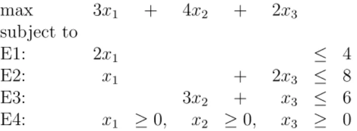
First we discuss how one recognize the optimality of a feasible solution. Let’s look at the Chateau Maxim problem.
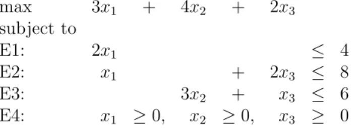
max 3x1 + 4x2 + 2x3
subject to
E1: 2x1 ≤ 4
E2: x1 + 2x3 ≤ 8
E3: 3x2 + x3 ≤ 6
E4: x1 ≥0, x2 ≥0, x3 ≥ 0
How can one convince someone (yourself, for example) that the production (Red 2, White 1 and Rose 3 units) is optimal?
(x1, x2, x3) = (2,1,3)
profit = 3×2 + 4×1 + 2×3 = 16
• Because we have checked many (say 100,000) feasible solutions and the production above is the best among them...
• Because CPLEX returns this solution and CPLEX is a famous (and very expensive) software, it cannot be wrong.
• We exhausted all the resources and thus we cannot do better.