Supervised classification with interdependent variables to support targeted energy efficiency measures in the residential sector

(1)

Supervised classification

with interdependent variables to support targeted energy efficiency measures in the residential sector

Mariya Sodenkamp^1*, Ilya Kozlovskiy¹ and Thorsten Staake^1,2

Background

Reducing energy consumption is the best sustainable long-term answer to the challenges associated with increasing demand for energy, fluctuating oil prices, uncertain energy sup- plies, and fears of global warming (European commission 2008; Wenig et al. 2015). Since the household sector represents around 30 % of the final global energy consumption (Inter- national Energy Agency 2014), customized energy efficiency measures can contribute sig- nificantly to the reduction of air pollution, carbon emissions, and economic growth. There is a wide range of potential courses of action that can encourage energy efficiency in dwellings, including flexible pricing schemes, load shifting, and direct feedback mechanisms (Sodenkamp et al. 2015). The major challenge is however to decide upon the appropriate energy efficiency measures in the circumstances when household profiles are unknown.

Abstract

This paper presents a supervised classification model, where the indicators of correlation between dependent and independent variables within each class are utilized for a transformation of the large-scale input data to a lower dimension without loss of recognition relevant information. In the case study, we use the consumption data recorded by smart electricity meters of 4200 Irish dwellings along with half-hourly outdoor temperature to derive 12 household properties (such as type of heating, floor area, age of house, number of inhabitants, etc.). Survey data containing characteristics of 3500 households enables algorithm training. The results show that the presented model outperforms ordinary classifiers with regard to the accuracy and temporal characteristics. The model allows incorporating any kind of data affecting energy consumption time series, or in a more general case, the data affecting class-dependent variable, while minimizing the risk of the curse of dimensionality. The gained information on household characteristics renders targeted energy-efficiency measures of utility com- panies and public bodies possible.

Keywords: Energy consumption, Household characteristics, Energy efficiency, Consumer behaviour, Pattern recognition, Multivariate analysis, Interdependent variables

Open Access

© 2016 Sodenkamp et al. This article is distributed under the terms of the Creative Commons Attribution 4.0 International License (http://creativecommons.org/licenses/by/4.0/), which permits unrestricted use, distribution, and reproduction in any medium, provided you give appropriate credit to the original author(s) and the source, provide a link to the Creative Commons license, and indicate if changes were made.

RESEARCH

*Correspondence:

Mariya.Sodenkamp@

uni-bamberg.de

1 Energy Efficient Systems Group, University of Bamberg, Bamberg, Germany

Full list of author information is available at the end of the article

(2)

In recent years, several attempts have been made toward mechanisms of recognition of energy-consumption-related dwelling characteristics. Particularly, unsupervised learning techniques group the households with similar consumption patterns in clusters (Figueiredo et al. 2005; Sánchez et al. 2009). Indeed, interpretation of each cluster by an expert is required. On the other hand, the existing supervised classification of private energy users relies upon the analysis of consumption curves and survey data (Beckel et al. 2013; Hopf et al. 2014; Sodenkamp et al. 2014). Hereby, the average prediction fail- ure rate with the best classifier (support vector machine) exceeds 35 %. The reasons for this low performance seem to stem from the fact that energy consumption is generally assessed in relation to a number of other relevant variables, such as economic, social, demographic and climatic indices, energy price, household characteristics, residents’

lifestyle, as well as cognitive variables, such as values, needs and attitudes (Beckel et al.

2013; Santos et al. 2014; Elias and Hatziargyriou 2009; Santin 2011; Xiong et al. 2014).

Practically, one can include all prediction-relevant data, independently on its intrinsic relationships, into a classification task in the form of features. This leads, however, to a high spatio-temporal complexity, and incurs a significant risk of curse of dimensionality.

In predictive analytics, the classification (or discrimination) problem refers to the assignment of observations (objects, alternatives) into predefined unordered homogene- ous classes (Zopounidis and Doumpos 2000; Carrizosa and Morales 2013). Supervised classification implies that the function of mapping objects described by the data into categories is constructed based on so called training instances—data with respective class labels or rules. This is realized in a two-step process of, first, building a prediction model from either known class labels or using a set of rules, and then automatically classifying new data based on this model.

In practice, the problem of finding functions with good prediction accuracy and low spatio-temporal complexity is challenging. Performance of all classifiers depends to a large extent on the volume of the input variables and on interdependencies and redun- dancies within the data (Joachims 1998; Kotsiantis 2007). At this point, dimensionality reduction is critical to minimizing the classification error (Hanchuan et al. 2005).

Feature selection is the first group of dimensionality reduction methods that identify the most characterizing attributes of the observed data (Hanchuan et al. 2005). More general methods that create new features based on transformations or combinations of the original feature set are termed feature extraction algorithms (Jain and Zongker 1997). Indeed, by definition all dimensionality reduction methods result in some loss of information since the data is removed from the dataset. Hence it is of great importance to reduce the data in a way that preserves the important structures within the original data set (Johansson and Johansson 2009).

In environmental and energy studies, the need to analyze large amounts of multivariate data raises the fundamental problem: how to discover compact representations of interacting and high-dimensional systems (Roweis and Saul 2000).

The existing prediction methods that treat multi-dimensional data include multivariate classification based on statistical models (e.g., linear and quadratic discriminant analysis) (Fisher 1936; Smith 1946), preference disaggregation (such as UTADIS and PREFDIS) (Zopounidis and Doumpos 2000), criteria aggregation (e.g., ELECTRE Tri) (Yu 1992; Roy 1993; Mastrogiannis et al. 2009), model development (e.g., regression

(3)

analysis and decision rules) (Greco et al. 1999; Srinivasan and Shocker 1979; Flitman 1997), among others. The common pitfall of these approaches is that they treat observations independently, and neglect important complexity issues. Correlation-based classification (Beidas and Weber 1995) considers influence between different subsets of measurements (e.g., instead of using both subsets correlation between them is computed and is then used instead), but use them as features only. The correlation-based classifier also does not consider the possibility of the correlation being dependent on class labels.

In this work, we propose a supervised machine learning method called DID-Class (Dependent-independent data classification) that tackles magnitudes of interaction (cor- relation) among multiple classification-relevant variables. It establishes a classification machine (probabilistic regression) with embedded correlation indices and a single normalized dataset. We distinguish between dependent observations that are affected by the classes, and independent observations that are not affected by the classes but influence dependent variables. The motivation for such a concept is twofold: first, to enable simultaneous consideration of multiple factors that characterize an object of interest (i.e., energy consumption affected by economic and demographic indices, energy prices, climate, etc.); and second, to represent high-dimensional systems in a compact way, while minimizing loss of valuable information.

Our study of household classification is based on the half-hourly readings of smart elec- tricity meters from 4200 Irish households collected within an 18-month period, survey data containing energy-efficiency relevant dwelling information (type of heating, floor area, age of house, number of inhabitants, etc.), and weather figures in that region. The results indicate that the DID-Class recognizes all household characteristics with better accuracy and temporal performance than the existing classifiers.

Thus, DID-class is an effective and highly scalable mechanism that renders broad analysis of electricity consumption and classification of residential units possible. This opens new opportunities for reasonable employment of targeted energy efficiency measures in private sector.

The remaining of this paper is organized as follows. “Supervised classification with class-independent data” describes the developed dimensionality reduction and classification method. “Application of DID-Class to household classification based on smart electricity meter data and weather conditions” presents application of the model for the data. The conclusions are in “Conclusion”.

Supervised classification with class‑independent data Problem definition and mathematical formulation

Supervised classification is a typical problem of predictive analytics. Given a training set N¯ =

¯ x1,y1

,. . .,

¯ xn,yn

containing n ordered pairs of observations (measurements)

¯

x_i with class labels y_i∈J and a test set M¯ = {¯x_n+1,. . .,x¯_n+m} of m unlabeled observations, the goal is to find class labels for the measurements in the test set M¯.

Let X¯ = {¯x_i} be a family of observations, and Y = {y_i} be a family of associated true labels. Classification implies construction of a mapping function x¯i�→f(x¯i) of the input, i.e. vector x¯i∈ ¯X, into the output, i.e. a class label yi.

(4)

A classification can be either done by a single assignment (only one class label y_i is assigned to one sample x¯i), or as a probability distribution over J classes. The latter algorithms are also called probabilistic classifiers.

Some elements of vector x¯_i can be differentiated, if they are not related to y_i. Let S= {s_i} be a subset of X¯ with s_i⊂ ¯x_i that are statistically independent from Y:

We define a family S of measurements s_i as independent. Simply put, observations s_i are not influenced by class labels y_i. The remaining observations are called dependent, and are defined as X= {x_i} with x_i = {z∈ ¯x_i|z∈/s_i}.

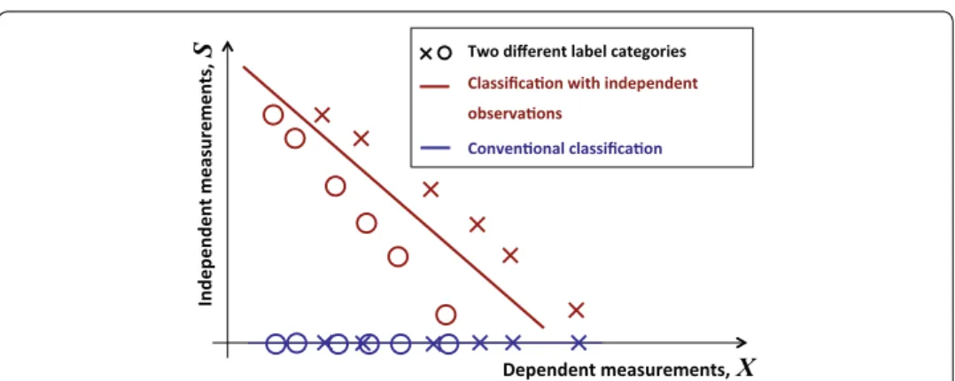
Independent variables can influence the dependent ones and thus be relevant for prediction. Figure 1 shows an example for this. The two different classes are represented by o and x. The x-axis shows the dependent variable, the y-axis the independent variable.

The objects in blue colour show that the classification with only the dependent variable would be impossible. On the other hand using both the dependent and independent data it is possible to linearly separate the two classes. For each independent value there are two observations with different class labels (i.e., the class label does not depend directly on S). On the other hand the class labels change depending on the values X, but only with combination of X and S do the classes become linearly separable.

We implement the given notation of dependent and independent variables in our DID- Class prediction methodology.

A training set N of DID-Class takes the form of the set of three-tuples:

A test set M is then extended to the ordered pairs:

Figure 2 visualizes relationships between variables in a conventional classification and in the DID-Class graphical model.

(1) P(y=j|s=z)=P(y=j),∀j∈J,z∈ {s1,. . .,sn}

(2) N=

x₁,s₁,y₁ ,. . .,

x_n,s_n,y_n .

M= {(x_n₊₁,s_n₊₁),. . .,(xn+m,s_n₊_m)}.

X

S

Fig. 1 Class partition with independent data and conventional classification

(5)

The DID‑class model

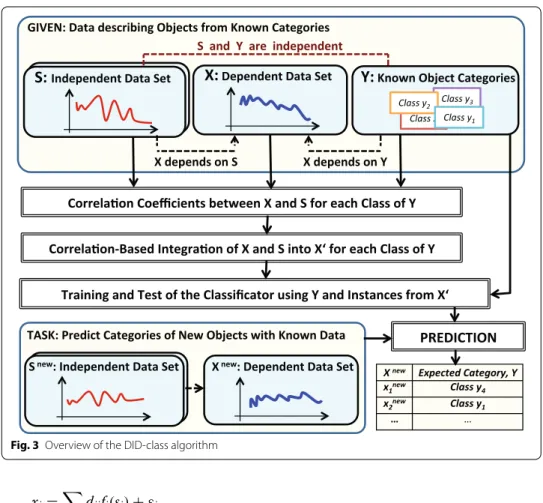
In this section we describe the proposed three-step algorithm in detail. In Fig. 3 we have attempted to capture the main aspects of the DID-Class model discussed in this section.

Step 1: Estimation of interdependencies between the datasets

DID-class is a method that makes use of the fact of relationships between input variables of the classification. Therefore, once the input datasets are available, it is necessary to test underlying hypotheses about associations between the variables. Throughout this note, the following two assumptions will be made.

Assumption 1 The independent variables S are statistically independent of the class labels Y, as defined by (1).

In other words, classification based on si is random.

Assumption 2 Independent variables S affect the dependent variables X and this influence can be measured or approximated.

Correlation coefficients can be found by solving a regression model of X expressed through regressors S and class labels Y.

DID-class relies upon the multivariate generalized linear model, since this formulation provides a unifying framework for many commonly used statistical techniques (Dobson 2001):

X = f (Y )

X = f (Y , S ) a

b

Fig. 2 Relationships between variables in conventional prediction (a) and in DID-Class (b)

(6)

The error term ε_i captures all relevant but not included in the model variables, because they are not observed in the available datasets. d_ij are the dummy variables for the class labels:

The most important assumption behind a regression approach is that an adequate regression model can be found (Zaki and Meira 2014). A proper interpretation of a linear regression analysis should include the checks of (1) how well the model fits the observed data, (2) prediction power, and (3) magnitude of relationships.

1. Model fit Depending on the choice of forecasting model and problem specifics, any appropriate quality measure [e.g., coefficient of determination R² or Akaike information criterion (D’Agostino 1986)] can be used to estimate the discrepancy between the observed and expected values.

2. Generalizing performance The model should be able to classify observations of unknown group membership (class labels) into a known population (training instances) (Lamont and Connell 2008) without overfitting the training data.

3. Effect size If the strength of relationships between the input variables is small, then the independent data can be ignored and application of DID-class is not necessary.

x_i= (3)

j∈J

d_ijf_j(s_i)+ε_i.

d_ij=

1 fory_i =j 0 fory_i�=j .

Fig. 3 Overview of the DID-class algorithm

(7)

The effect size is estimated in relation to the distances between classes using appropriate indices (e.g., Pearson’s r or Cohen’s f²).

The functions fj describe how the dependent variables can be calculated from the independent ones and class labels. These functions are utilized in later steps of the presented algorithm to normalize response measures and eliminate predictor variables. The unknown functions f_j are typically estimated with maximum likelihood approach in an iterative weighted least-squares procedure, maximum quasi-likelihood, or Bayesian techniques (Nelder and Baker 1972; Radhakrishna and Rao 1995). Thus, a unique fj is set in a correspondence to each class j∈J. A single relationship model can be built for the set of all classes, by adding dummy variables of these classes.

If X linearly depends on S, then (3) can be rewritten as follows:

Correlation coefficients α and β can be calculated using the ordinary least squares method. If the relationships are not linear, then a more complex regression model can be used. For instance, for the polynomial dependency, variables with powers S can be added on the right side of Eq. (4). In this case, networks with mutually dependent variables can be taken into account, as shown in Fig. 2.

Step 2: Integration of dependent and independent measurements

In order to take the correlation coefficients revealed on the previous step into consideration, and transform the multivariate input data to a lower dimension without loss of classification-relevant information, we normalize the dependent variables with respect to the independent ones. Normalization means elimination of changes in the dependent measurements that occur due to the shifts in the independent values, and transformation of X into X^′.

Since the relationships of X and S are different for each class, the normalization is also class-dependent. Each measurement x_i in the training set N is normalized according to the corresponding class label y_i.

Model (3) expresses regression for each single class label. f_j are used as the normaliza- tion functions. The normalized training set takes the following form:

with

Every x^′_i is the normalized representation of the dependent measurement x_i. The term f_y_i(s_i)−f_y_i(s₁) describes the expected difference between s_i and s₁, by the chosen regression model. Hereby, s₁ is the default state and no normalization is needed for xiwithsi =s1. As a result, there are a normalization functions for a class labels. Without loss of generality, any value can be chosen as the default value. However, a data-specific value may allow for better interpretation of the results.

x_i= (4)

j∈J

d_ij(α_j+β_j×s_i)+ε_i.

(5) N^′=

x₁^′,y₁ ,. . .,

x^′_n,y_n

x^′_i=x_i−f_y_i(s_i)+f_y_i(s₁).

(8)

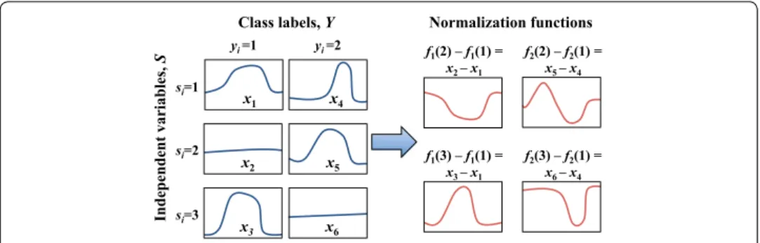
Figure 4 provides a simple example for the normalization, where dependent measurements are time series that must be classified between two categories. Additionally, there is a discrete independent variable with 3 possible values. In this case, the normalization functions can be computed as the difference of the time series.

Step 3: Classification

Once all classification-relevant input datasets are integrated into one normalized set, it can be used as an input for a probabilistic classifier (further referred to as C) that returns distribution probability over the set of class labels.

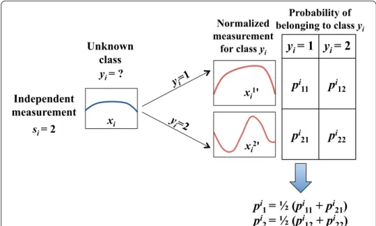
To enable prediction of the class for a new observation it is necessary to normalize its value. The challenge is however to choose the appropriate normalization function f_j from the a functions constructed on the step 1. But since the class labels for the test data are unknown, there is no a priori knowledge on which normalization function should be used. It is possible to apply any fj, but the classification is more likely to be successful if the correct f_j was chosen (i.e., the test data belongs to the class from which the normalization function was derived). Therefore, DID-class tests all functions for a new observation and chooses the solution with the highest probability for each individual class. After that, the test-set-measurement is transformed and classified a times. Finally, the averages of the resulting probabilities for each class are derived. The observation belongs to the class with the highest resulting probability.

The prediction process is formally described below.

A normalized measurement is derived for each unlabeled element and each class. The test set takes the following form:

where

This transformed test set is used as in input of the trained probabilistic classifier C that is chosen at the beginning of Step 3. Its output is a probability vector of a values for each

{x^j_i^′}i∈{n+1,...,m},j∈J

x^j_i^′ =x_i−f_j(s_i)+f_j(s₁).

y_i=1 y_i=2 s_i=1

s_i=2

s_i=3

f₁(2) –f₁(1) =

x₂– x₁ f₂(2) – f₂(1) = x₅– x₄ x1

x₂ x₃

x4

x₅ x₆

f₁(3) – f₁(1) =

x₃– x₁ f₂(3) – f₂(1) = x₆–x₄ Class labels, Y Normalization functions

Independent variables, S

Fig. 4 An example of normalization functions construction

(9)

normalized measurement. Thus, the following probability matrix is set to each unlabeled value in correspondence:

where pⁱ_kl designates the probability of element x_i to belong to the class l after normalization according to the class k. Prediction of the class label of x^j_i^′ is naturally biased for

j , but this is compensated by the prediction being done for all a classes. The aggregated probability for class l is Pⁱ_l = ^Σ^k^p

i kl

a .

This process results in a probabilistic classifier for the measurements from the test set.

We can also label the measurements as belonging to the class with the greatest probability. The resulting figures P_lⁱ are biased probabilities of element i belonging to class l , which means that DID-Class should be used as a non-probabilistic classifier. Figure 5 visualizes an example of the classification step for two class labels.

Temporal complexity of classification depends on the dimension of included variables (Lim et al. 2000).

Classification training with DID-Class uses normalized set N^′ with n variables of dimension d_x. A classification without DID-Class would use the initial training set N, with the dimension of d_x+d_s, where d_x and d_s stand for the dimensions of variables in X and S respectively.

The prediction using DID-Class is done for a×n variables with dimension d_x. A classification without DID-Class would be done for only n variables, but with higher dimension, namely d_x+d_s. Hence, DID-Class can perform better or worse than a classifier that analyzes all data in its initial form (without correlation information), depending on the number of categories a and dimension of independent variables. Particularly, DID- class is more efficient compared to the algorithms where training complexity is higher

Pⁱ=

pⁱ_kl

{^k,l∈J}

y

_i

= 1 y

_i

= 2 p

ⁱ₁₁

p

ⁱ₁₂

p

ⁱ₂₁

p

ⁱ₂₂ y_i= ?

x_i

p

ⁱ₁

= ½ (p

ⁱ₁₁

+ p

ⁱ₂₁

) p

ⁱ₂

= ½ (p

ⁱ₁₂

+ p

ⁱ₂₂

)

Unknown

class Independent

measurement si = 2

xi1'

xi2' Normalized measurement

for class y_i

Probability of belonging to class y_i

Fig. 5 Example of probability distribution over classes for an unlabeled time series calculated by DID-class

(10)

than the prediction complexity, which is valid for the majority of commonly used classi- fiers (e.g., support vector machines (SVM), Adaboost, Random Forest, Linear Discrimi- nant Analysis, etc.).

The proposed algorithm is described in Table 1.

Verification of DID‑class

In this section, we show that the proposed methodology yields linearly separable categories of objects, under the specified conditions.

Theorem 1 Let N be the training set of a classification problem as described by Eq. (2).

Further suppose that the model for the dependency (3) of S on X is known (i.e., the functions f_j are known in advance) and let δ be an upper bound on the errors ε_i in the model:

Let then N^′ be the training set normalized with the correct functions (5).

If there exists an index l_j for each class label j∈J, such that the distance between the chosen normalized measurements is greater than 4δ

then the classes in the normalized training set are linearly separable.

δ=max (6)

i �x_i−f_y_i(s_i)�.

�x^′_l

1−x^′_l

2 �>4δ, ∀l₁,l₂∈ l_j

j∈J,l₁�=l₂,

Table 1 The algorithm of DID‑Class

Input: training data set {(x1,s1,y1),. . .,(xn,sn,yn)} and test examples {(xn+1,sn+1),. . .,(xn+m,sn+m)} Output: probability distributions

Pⁿ⁺¹,. . .,P^n+m

over the classes

1. Show that the correlation between independent and dependent measurements exists 2. Show that the independent measurements are not affected by the class labels

3. Compute the influence (fj) of different independent measurements on distinct class labels, by solving the generalized linear model

4. xi=

j∈J

d_ijf_j(s_i)+εi

5. For each i∈ {1,. . .,n} compute the normalized measurements:

6. x_i^′=x_i−f_y_i(s_i)+f_y_i(s1)

7. Create the probabilistic classifier C with the training set x₁^′,y1

,. . ., x_n^′,y_n 8. For each i∈ {n+1,. . .,n+m}

9. For each j∈J compute the normalized measurements for unlabelled data as each possible class 10. x_i^j^′=x_i−f_j(s_i)+f_j(s1)

11. Apply the classifier C to the normalized measurements 12. ∀k∈Jletpⁱ_jk:= probability of x^j_i^′ belonging to class k 13. Let P_lⁱ= ^Σ^k^p

i kl

a be the probability of xi belonging to class l 14. Return

Pⁿ⁺¹,. . .,P^n+m

(11)

Proof All the normalized measurement of a single class j are contained in the 2δ-neigh- borhood of the normalized measurement x^′_l

j since, for yi=j:

This means that every normalized measurement for different classes is contained in a convex compact ball of radius 2δ centered on the normalized measurements x_l_j. The different balls are disjoint since the distance between the centers of the balls is greater then 4δ, and therefore the distance between balls is greater than 0. Hence there exists a hyper-

plane separating any two classes.

An analogous statement can be proven if the model is unknown, but the kind of dependency is known. The estimation of errors in this case is inherent to the model.

Theorem 2 proves this statement for the case of linear dependency. Other regression models can be treated in a similar manner.

Theorem 2 Let N be the training set of a classification problem as described by Eq. (2).

Further suppose that the model (3) is unknown (i.e., the functions f_j have to be estimated based on the data), and let δ be an upper bound on the error ε_i in (6).

If there exists an index lj for each class label j∈J, such that the distance between the chosen normalized measurements is greater than 4√

nδ

then the classes in the normalized training set are linearly separable.

Proof Let f_j^′ be the estimated functions of the linear model. The sum of squared errors for the estimated model is bounded by the sum of squared errors for the actual model:

Therefore we get an upper bound for a single error in the estimated model:

�x^′i−x^′_l_j � = �xi−fj(si)+fj(s1)−x_l_j +fj

s_l_j

−fj(s1)�

= �x_i−f_j(s_i)−x_l_j+f_j s_l_j

�

≤ �xi−fj(si)� + �x_l_j−fj

s_l_j

�

≤ δ+δ

=2δ.

�x^′_l

1−x^′_l

2 �>4√

nδ, ∀l₁,l₂∈ l_j

j∈J, l₁�=l₂,

il

�xi−f_y^′_i(si)�²≤

i

�xi−f_y^′_i(si)�²≤nδ.

�x_i−f_y^′_i(s_i)�²≤

i

�x_i−f_y^′_i(s_i)�²≤nδ²

�xi−f_y^′_i(si)�≤√ nδ.

(12)

Analogously to the proof of Theorem 1 we can now show, that each normalized measurement of the class j is contained in the 2√

nδ neighbourhood of the normalized measurement x_l_j′ :

This means that every normalized measurement for different classes is contained in a convex compact ball of radius 2√

nδ centered on the normalized measurements x_l_j. The different balls are disjoint since the distance between the centers of the balls is greater then 4√

nδ, and therefore the distance between balls is greater than 0. Hence there exists a hyperplane separating any two classes.

We have shown that if (a) Assumptions 1 and 2 are satisfied, (b) regression model describing relations of input variables is reasonable, and (c) different classes are far from each other, then the normalized training set yielded by DID-Class is a linearly separable set.

Application of DID‑Class to household classification based on smart electricity meter data and weather conditions

In this section we present a classification of residential units based on smart electricity meter data and weather variables by DID-Class. Results indicate that DID-Class outperforms the best existing classifier with regard to the accuracy and temporal characteristics.

Data description

Our study is based on three following samples.

(a) The power consumption data of 30-minutes granularity that originates from the Irish Commission for Energy Regulation (CER) (ISSDA. Data from the commission for energy regulation 2014). It was gathered during a smart metering trial over a 76-week period in 2009–2010, and encompasses 4200 private dwellings. It is a dependent data set X, according to the definition given in “Problem definition and mathematical formulation”.

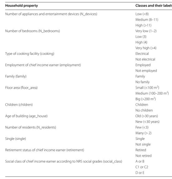
(b) The respective customer survey data containing energy-efficiency-related attributes of households (such as type of heating, floor area, age of house, number of residents, employment, etc.). It is a data set of known object categories Y, according to the definition given in “Problem definition and mathematical formulation”. For the classification problem we consider 12 different household properties, which are presented on the left hand side of Table 2. The classification is made for each property individually.

The properties can take different values (“class labels”) that are presented on the right hand side of Table 2. For example, each household can be classified as either “electri-

�x^′_i−x_l^′

j � = �x_i−f_j^′(s_i)+f_j^′(s₁)−x_l_j +f_j^′ s_l_j

−f_j^′(s₁)�

= �x_i−f_j^′(s_i)−x_l_j+f_j^′

s_l_j

�

≤ �x_i−f_j^′(s_i)� + �x_l_j−f_j^′ s_l_j

�

≤ √ nδ+√

nδ

= 2√ nδ.

(13)

cal” or “not electrical” with respect to the property “type of cooking facility”. The con- tinuous values are divided into discrete intervals [e.g., property “age of building” is expressed by two alternative class labels “old”(>30 years) and “new” (≤30 years)]. For three household properties “age of house”, “floor area” and “number of bedrooms”

the discrete class labels were defined according to the training data (surveys). For the properties “number of residents” and “number of devices”, the classes were defined to have a roughly equal distribution of households (Beckel et al. 2013).

(c) Multivariate weather data, including outdoor temperature, wind speed, and precipi- tation of 30-min granularity in the investigated region provided by the US National Climatic Data Center (NCDC 2014). It is an independent multivariate data set S, where S₁=outdoor temperature, S₂=wind speed, and S₃=precipitation.

In the current implementation, we assume that an observation refers to a 1-week data trace (including weekend), because it represents a typical consumption cycle of inhabitants. One week of data at a 30-min granularity implies that an input trace contains 336 data samples for each variable.

Table 2 The properties and their class labels

Household property Classes and their labels

Number of appliances and entertainment devices (N_devices) Low (<8) Medium (8–11) High (>11)

Number of bedrooms (N_bedrooms) Very low (1–2)

Low (3) High (4) Very high (>4)

Type of cooking facility (cooking) Electrical

Not electrical

Employment of chief income earner (employment) Employed

Not employed

Family (family) Family

No family

Floor area (floor_area) Small (<100 m²)

Medium (100–200 m²) Big (>200 m²)

Children (children) Children

No children

Age of building (age_house) Old (>30 years)

New (<30 years)

Number of residents (N_residents) Few (<3)

Many (> 2)

Single (single) Single

Not single Retirement status of chief income earner (retirement) Retired

Not retired Social class of chief income earner according to NRS social grades (social_class) A or B

C1 or C2 D or E

(14)

Since the CER data set does not contain any facts about household locations or about the geographical distribution of households, we calculated the average of independent variables over all 25 weather stations in Ireland

Prediction results

In the present study, we split the input data into training and test cases in the proportion 80–20 %. The training instances are used to estimate the interdependencies between electricity consumption and outdoor temperature and then train the classifier. The test instances are then used to evaluate accuracy of the classification results.

Step 1: Influence estimation

First, we check if Assumptions 1 and 2 hold for the given variables.

Assumption 1 The condition of independency of weather (S) from household properties (Y) is trivially satisfied, since the weather is equal for all dwellings.

Assumption 2 A regression model must be found to approximate the influence of weather (S) on energy consumption (X).

A lot of work has been done on electricity demand prediction and therefore also modeling of the energy consumption based on external factors (e.g., weather) (Zhongyi et al. 2014; Veit et al. 2014; Zhang et al. 2014). In the present study to show the application of the method we will construct only a simple linear regression model for electricity consumption and corresponding outdoor temperature. Previous studies showed a major relation of power consumption and temperature (Apadula et al. 2012; Suckling and Stackhouse 1983). Therefore, we start constructing a regression based on these two variables. In housing situations with air conditioning energy consumption is lowest at the temperature range 15–25 °C and increases for both then the temperature increases, due to the air conditioning devices and then the temperature decreases, due to heating devices. Due to the medium climate in the region under consideration, there are typically no air conditioners in private households (Besseca and Fouquaub 2008), this is why the linear approximation for power consumption as given below is justified.

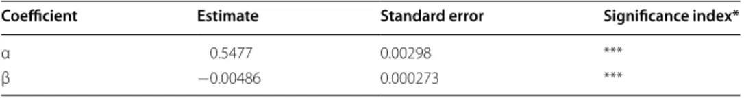
Results of (7) are summarized in Table 3. The model fit of R²=0.13 is acceptable, where R² is the coefficient of determination and is defined as the percentage of total variance explained by the model (Radhakrishna and Rao 1995). R²∈ [0, 1] and R²=1

(7) X=α+β×S₁+ε.

Table 3 Coefficients in the linear regression model (7)

* Significant at <5 %

** Significant at <1 %

*** Significant at <0.1 %

Coefficient Estimate Standard error Significance index*

α 0.5477 0.00298 ***

β −0.00486 0.000273 ***

(15)

reflects a perfect model fit. Further, we observe that increase of temperature by 1 °C leads to a drop in consumption by 0.00486 kWh for an average household, which is only 0.9 % of the average consumption during the corresponding half-hour period. Hence, average diurnal temperature change of 8° leads to an increase of energy consumption by 7 %. Even a greater seasonal effect is observed between summer and winter, where mean differences of up to 15 °C can be expected. This leads to the relative change of 13 % in power usage.

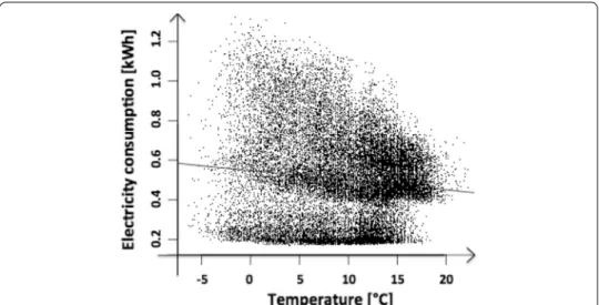
The regression results are visualized in Fig. 6. It reflects a negative correlation between the consumption and outdoor temperature.

Model (7) has a slight bias for the positive correlation, which can be explained by the fact that values of both variables are lower during the night. This is accounted for by computing the model for each time stamp separately (i.e., “00:00”, “00:30”,…, “23:30”).

The results are summarized in Table 4. The detailed results are presented in Additional file 1.

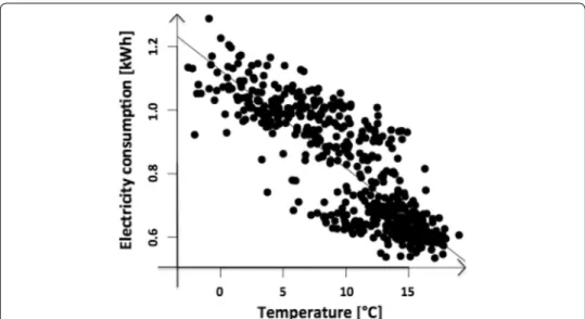
The temperature impact is highly significant for each hour of the day, but the influence is much stronger in the evening hours, and the value of R² attains the highest value of 0.7313 between 18:00 and 20:00. This influence is visualized in Fig. 7. Usage of heating devices that are active at low temperatures is a probable explanation of this correlation.

Fig. 6 Scatterplot of temperature and energy consumption with regression line

Table 4 Coefficients in model (7) for different times of the day

Time R² β Sig. Ind.

05:00 0.2142 −0.0016 ***

09:00 0.3691 −0.0069 ***

19:00 0.7135 −0.0391 ***

(16)

Besides the actual air temperature, the apparent temperature is an important indica- tor affecting energy consumption by individuals. Therefore, we add this influence in the model (7). Apparent temperature depends on the relative humidity and wind speed. Due to the lack of high-quality observations for relative humidity we only consider a wind speed component (S₂). As a result, (7) can be rewritten as follows:

The results of (8) are summarized in Table 5. This model improves R² to 0.2257. The coefficients for temperature and wind speed are close, but the standard error is larger.

Since the typical range of values is smaller for wind speed, its effect size on consumption is also smaller.

The half-hour results of model (8) are presented in Table 6. The influence of wind speed is much lower than that of the temperature and the coefficients β₂ are mostly not significant, except evening hours where R² attains its maximum value.

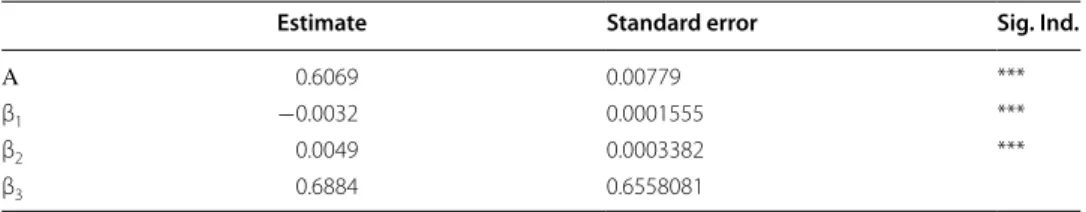
At the final stage of relationships estimation, we add daily precipitation (S₃) to (8). This variable has two special properties: first, its values are only available at a daily granularity; second, there are two different kinds of precipitation—rain and snow—that may have different effects on energy consumption. Nevertheless, we use an aggregate precipitation variable and compute the following linear model:

(8) X=α+β₁×S₁+β₂×S₂+ε.

(9) X=α+β₁×S₁+β₂×S₂+β₃×S₃+ε.

Fig. 7 Scatterplot of temperature and energy consumption with regression line at 7 p.m

Table 5 Summary of model (10)

Estimate Standard error Sig. Ind.

α 0.5013 0.00405 ***

β₁ −0.00589 0.00028 ***

β₂ 0.00527 0.00031 ***

(17)

The results are summarized in Table 7.

The coefficient β₃ for daily precipitation is not significant. The values of daily precipitation vary minimally—between 0 and 0.02 mm per 30 min.

To summarize, we have shown that temperature is a strong predictor of energy consumption. Moreover, the prediction power also depends on the time of the day. Other factors, like wind speed and precipitation, are less relevant in predicting energy demand.

Step 2: Integration of dependent and independent measurements

Based on the results of previous step, we choose predictor (7) and consider different times of the day.

Further the model (7) is completed with dummy variables for different classes:

We expect the influence of weather to be notably different for at least some class labels (e.g., households with large floor area or many residents use more heating energy).

We use mean temperature as the default independent measurement (s₁) for normalization. This way the normalized consumption values correspond to the consumption expected at mean temperature.

Step 3: Classification

At this step, we compare accuracy and temporal complexity of DID-class with SVM, and then with CLASS (Beckel et al. 2013).

1. Comparison of DID-class with a baseline classifier.

First, we show the advantages of the DID-Class method over a Naïve classification with respect to the accuracy and runtime complexity. As a Naïve classification, we x_i=

j∈J

d_ij

α_j+β_j×s_1i +ε_i.

Table 6 Summary of model (8) for different hours

R² β₁ Sig. Ind. for β₁ β₂ Sig. Ind. for β₂

09:00 0.369 −0.0039 *** 0

19:00 0.7387 −0.0223 *** 0.0082 ***

05:00 0.2337 −0.0009 *** 0.0005 ***

Table 7 Result of the complete linear model (9)

Estimate Standard error Sig. Ind.

Α 0.6069 0.00779 ***

β₁ −0.0032 0.0001555 ***

β₂ 0.0049 0.0003382 ***

β₃ 0.6884 0.6558081

(18)

consider one that simply uses all observation variables as features [i.e., it tries to find the classification function f with Y = f(X,S)]. We have chosen SVM as a baseline classifier for comparison, because it is currently the best-known algorithm for prediction of energy-efficiency related characteristics of residential units (Beckel et al. 2013). To ensure objective comparison, we first tuned SVM to achieve the best accuracy, and only then used this SVM version in the core of DID-class.

Since the independent variables (weather) are identical for all households for each observation (1 week), considering these variables will not have influence on the single- week classification results based on a conventional algorithm (with weather taken as features). To cope with this challenge, it is possible to include several observations into analysis. In our experiments, we used the data from three consecutive weeks for the training of both baseline classifier and DID-class. Moreover, we repeated the comparison for four different timespans to ensure stability of the results. These (calendar) weeks are: 47–49 (November) in 2009, 5–7 (January–February) in 2010, 11–13 (March–April) in 2010, and 31–33 (August) in 2010. The comparison results are shown in Table 8. It can be seen, that DID-Class performs either better or the same on all runs.

For clarity reasons, we calculated the average accuracy on four runs. Table 9 (col- umns 2–3) indicates that DID-Class achieves better accuracy for 11 out of 12 properties, and the same accuracy for only one property (“cooking”). In other words, DID- class reduces the error rate by 2.8 % on average, maximum by up to 5.6 % for the property “retirement”.

A single experiment computations by SVM took 95 min on average, while the classification by DID-class on average took 25 min on the same laptop with 1.7 GHz Intel Core i7 CPU and 8 GB 1600 Hz RAM. The asymptotic complexity is O(n³) for both algorithms, but large dimension of the training set raises the runtime of SVM classifier (Sreekanth et al. 2010).

2. Comparison of DID-class with the state-of-the-art household classifier called CLASS (Beckel et al. 2013).

Table 8 Results with SVM (S) and SVM‑based DID‑class (SD)

Italic values indicate the highest classification accuracy

Property Weeks Weeks Weeks Weeks

47–49/09 05–07/10 11–13/10 31–33/10

S SD S SD S SD S SD

Single 80.1 81.1 80.6 81.6 80.4 81.4 79 79.8

N_devices 50.7 50.9 50.8 51 50.7 50.8 50.6 50.8

Cooking 73 73 72.7 72.8 72.5 72.5 73.3 73.3

Family 75 75.8 75.7 76.4 75.9 76.8 75.6 76.3

Children 74 74.6 73.7 74.4 74.7 75.3 73.6 74.1

Age_house 56.7 57.9 57.9 59.2 57.4 58.4 57.1 58.4

Social_class 50.5 50.8 51.8 52.3 51.1 51.3 50.5 50.6

Floor area 62.9 64.1 62.8 64.1 63.6 64.6 61.8 63

N_residents 71.4 72.6 71.3 72.4 69.9 71.1 71.9 73.1

N_bedrooms 48.2 49.2 47.8 48.9 48.6 49.7 49.3 50.3

Employment 66.8 67.8 66.9 67.9 65.9 67 66.2 67.2

Retirement 69.9 71.5 70.1 71.7 71.2 72.8 71.2 72.8

(19)

In their work, Beckel et al. (2013) applied SVM tuned with feature extraction and selection. The algorithm run on the calendar week number 2 in 2010. For comparison reasons, we use the same data and the same SVM version in the core of DID- Class.

Similarly to the previous case, we repeat the experiment four times and average the results (see Tables 9 and 10). The results shown in Table 8 indicate that DID-Class improves the classification accuracy on 1–3 % compared to the CLASS algorithm.

Especially floor area can be predicted more precisely, which seems to be natural because a larger household requires more heating at cold temperatures.

In both cases, DID-Class performs better.

Conclusion

Findings suggest that targeted feedback doubles the energy savings from smart metering from 3 percent of conventional systems to 6 percent when targeted feedback is used (Loock et al. 2011). This amounts to an additional efficiency gain of about 100 kWh per year and household, with its beauty being the scalability to virtually all households with of-the-shelf smart metering systems. Moreover, the tools allow for allocating resources for energy conservation and load shifting campaigns to households given their characteristics are known.

This research goes beyond the state-of-the-art by providing a method to effectively reduce the dimensionality of the consumption data time series and additional power- usage-relevant data (e.g., weather, energy price, GDP, holidays and weekends, etc.) while minimizing information losses and enhancing accuracy of results, which forms a corner stone of subsequent policy analysis through personalized smart-metering-based interventions on a usable level.

The satisfactory performance of the DID-Class method in the validation datasets illus- trates its ability to classify potentially any household equipped with smart electricity Table 9 The average classification results as accuracy in % for each class

Property Comparison with trivial approach Comparison with the best known household classifier

SVM DID‑Class with SVM CLASS DID‑class with CLASS

Single 79.9 80.8 83.3 83.5

N_devices 50.6 50.8 52.9 53.5

Cooking 72.9 72.9 72.7 73

Family 75.1 75.9 77.1 77.6

Children 73.9 74.5 74.5 74.8

Age_house 56.9 58.1 61.5 61.6

Social_class 50.7 51 50.9 51.3

Floor area 62.9 64.1 63.5 65.2

N_residents 71.7 72.9 72.8 73.8

N_bedrooms 48.3 49.3 49.2 49.5

Employment 66.7 67.8 68.3 69.2

Retirement 70.1 71.7 71.9 72.7

(20)

meter. Additionally, any energy-consumption related data can be encompassed and contribute to the performance elevation.

The developed model could also be used for other classification problems with available “external” information. For instance, license plate recognition based on images from highway cameras, with illumination conditions and current daytime as independent variables, or credit scoring based on customer information, credit history, and loan appli- cations with additional information on economic values like GDP, unemployment rate, price index as independent observations.

Future research can be directed toward extension of the model to the cases with specific non-linear relationships between the pairs of dependent and independent variables.

Additionally future research could enhance DID-class toward extension of the set of properties, integration of other energy consumption figures (gas and warm water), combinations with other methods (multidimensional scaling, Isomap, diffusion maps, etc.

(Lee et al. 2010)), and development of a tool for a real-world setting. In the long-term, empirical validation of targeted interventions made by using the gained information could show the value of the developed methodology and tool.

Nomenclature

a: Number of different class labels; C: Classifier; d: dummy variables; f_j: normalization function for class j; J: set of all possible class labels; M¯,M: unlabelled test set; m: number of elements in the test set; N¯,N: labelled training set; N^′: normalized training set; n: number of elements in the training set; pⁱ_kl: probability of x^k_i^′ to belong to class l; Pⁱ_j: probability of xi

to belong to class j; S: family of all independent measurements; si: independent measurement; ¯xi: measurement; xi

: dependent measurement; x^′_i: normalized measurement xi; x_i^j^′: measurement xi normalized as class j; X: Family of all ¯ measurements; X: family of all dependent measurements; X^′: family of the normalized dependent measurements; Y: family of all class labels; y_i: class label.