Are Competitors Forward Looking in Strategic Interactions? Evidence from the Field

IHS Economics Series Working Paper 319

November 2015

Are Competitors Forward Looking in Strategic Interactions? Evidence from the Field

Mario Lackner

Rudi Stracke

Uwe Sunde

Rudolf Winter-Ebmer

Impressum Author(s):

Mario Lackner, Rudi Stracke, Uwe Sunde, Rudolf Winter-Ebmer Title:

Are Competitors Forward Looking in Strategic Interactions? Evidence from the Field ISSN: Unspecified

2015 Institut für Höhere Studien - Institute for Advanced Studies (IHS) Josefstädter Straße 39, A-1080 Wien

E-Mail: o ce@ihs.ac.atffi Web: ww w .ihs.ac. a t

All IHS Working Papers are available online: http://irihs. ihs. ac.at/view/ihs_series/

This paper is available for download without charge at:

https://irihs.ihs.ac.at/id/eprint/3797/

Are Competitors Forward Looking in Strategic Interactions? Evidence from the Field ^∗

Mario Lackner

, Rudi Stracke

, Uwe Sunde

, and Rudolf Winter-Ebmer

a

Department of Economics, University of Linz (JKU)

b

Department of Economics, University of Munich (LMU)

c

Institute for Advanced Studies (IHS), Vienna November 28, 2015

Abstract

This paper investigates empirically whether decision makers are forward looking in dynamic strategic interactions. In particular, we test whether decision makers in multi-stage tournaments take heterogeneity induced changes of continuation values and the ability of their immediate opponent into account when choosing effort. Using data from professional and semi-professional basketball tournaments, we find that effort is negatively affected by the ability of the current opponent, consistent with the theoretical prediction and previous evidence. More importantly, the results indicate that the expected relative strength in future interactions does affect behavior in earlier stages, which provides support for the ‘standard’ view that decision makers are forward looking in dynamic strategic interactions.

JEL Classification: D84; D90; M51; J33

Keywords : Promotion tournament; multi-stage contest; elimination; forward-looking be- havior; heterogeneity

∗Corresponding author: Uwe Sunde, Seminar for Population Economics, Department of Economics, Geschwister-Scholl-Platz 1, D-80539 M¨unchen; Tel.:+49-89-2180-1280; Fax:+49-89-2180 17834; Email:

uwe.sunde@lmu.de. Thanks to Alex Ahammer for help with the data and Josh Angrist, Jen Brown, Florian Englmaier, Dylan Minor, Steve Stillman and seminar participants in Ohlstadt, Laax, Vienna, Istanbul and Mannheim for helpful comments.

1 Introduction

Dynamic strategic interactions characterize many situations of economic decision making.

Modern macro models typically assume that decision makers are rational and forward looking, incorporating the consequences of future interactions in their current decisions.

Likewise, many contexts studied in microeconomics involve strategic and dynamic com- ponents. Obviously, this is motivated by the prevalence of such decision environments in reality. One prominent example are workplace interactions, where workers interact with their employer as well as with their co-workers repeatedly, with important implications for work incentives. A prime example of how these dynamic strategic interactions work and how they are incorporated in the design of employment relations are promotion tour- naments. Promotion tournaments are a common way of creating incentives for workers to exert effort on their job, but conceptually very similar tournaments are also observed in many other contexts, for instance during electoral competitions in majority voting systems, or in multi-stage procurement tournaments with shortlists.

The power and usefulness of tournament models for gaining a better understanding

of behavior in such strategic interactions has been demonstrated by the seminal work

of Lazear and Rosen (1981). While this benchmark model is essentially static, subse-

quent contributions highlight the importance of forward-looking behavior for optimal

effort choices in tournaments. In particular, Waldman (1984) assumes that competing

workers anticipate the signal value of a promotion for future wage negotiations, while

Rosen (1986) argues that the continuation value of future promotion possibilities is an

important determinant of current effort choices. Both approaches share the idea that the

next promotion is not the ultimate goal, but rather a means to an end of forward-looking

agents, namely either the prerequisite for future promotions to even more attractive posi-

tions within the same organization, or a signal observable by competing organizations that

then allows workers to demand higher wages. Apart from the few exceptions discussed

below, however, there is little to no evidence whether decision makers are indeed forward

looking in dynamic strategic interactions as typically assumed in theoretical models, even

though the existence and extent of forward-looking behavior is essential for many practical

purposes.

This paper provides evidence on this question by investigating how current hetero- geneity and the expected relative strength in future interactions affect behavior in dy- namic strategic interactions. A canonical multi-stage pairwise elimination tournament model predicts the well-known adverse incentive effect of heterogeneity according to which greater heterogeneity in a given interaction reduces effort of favorites and underdogs – in- dependent of whether decision makers are forward looking or not. The consideration of multiple stages delivers the additional prediction that the expected relative strength in future interactions has a positive effect on effort in a given (current) interaction if and only if decision makers are forward looking and take the continuation value into account.

However, whether and to what extent this is the case has not been tested systematically in the existing literature. The dynamic incentive effect due to forward-looking behavior is driven by the prospects of the higher expected winning odds in the next round that a competitor tries to take advantage of by increasing current effort. Using data from professional and semi-professional basketball tournaments, we then test whether or not tournament participants are forward looking. In particular, we consider the playoffs of NBA and NCAA basketball tournaments, which provide an ideal setting for this purpose.

On the one hand, these tournaments involve considerably large stakes, and, on the other hand, they provide precise information about all required elements, such as heterogeneity, effort and outcomes. Moreover, the differences between the NBA and NCAA tournament rules allow cross-validating the empirical findings.

Our findings support the view that decision makers are indeed forward looking. In particular, the results show that, everything else equal, the expectation of a weaker future opponent increases effort in the current match. The empirical results also suggest that the strategic aspect implied by the expectation of a weaker future opponent becomes more important the shorter the remaining tournament and the more pivotal the current game is, i.e. the closer the final interaction in the tournament. In addition, we find that effort is negatively affected by the ability of the current opponent, consistent with the theoretical prediction and previous evidence based on static interactions.

This paper contributes to, and extends, the existing literature on tournaments in

several ways. First, we contribute to existing work that investigates the effects of het-

erogeneity on behavior in static tournaments, see, e.g., Baik (1994). Empirical work that

tests these predictions has typically relied on data from lab experiments (see, e.g., Bull et al., 1987, Chen et al., 2011), and only few papers have investigated the role of hetero- geneity using field data from sports, see, e.g., Sunde (2009), Brown (2011), and Berger and Nieken (2014). Our work complements this literature by showing that static incen- tive effects of heterogeneity continue to matter in each stage of a multi-stage tournament structure. Second, this paper provides a direct test of a necessary condition of models with mechanisms that are based on dynamic implications, including models by Waldman (1984) and Rosen (1986), according to which the prospect of better outside options or of future promotions affects effort provision in earlier stages of the tournament. In par- ticular, we show that heterogeneity induced changes of continuation values affect effort choices of tournament participants, in line with the standard assumption that decision makers are indeed forward looking in dynamic strategic interactions. Thereby, this paper complements recent work that has investigated related issues in the lab, see, e.g., Alt- mann, Falk, and Wibral (2012) or Stracke and Sunde (2015). Evidence from the field is scarce, however. A notable exception is work by Delfgaauw, Dur, Non, and Verbeke (2015) who implement a two-stage elimination tournament in a field experiment. They focus on the effect of variations in the structure of prizes and in the importance of noise within a given stage, not on the effect of continuation values across stages as done here.

To our knowledge, the only study that indirectly accounts for dynamic incentive effect in multi-stage tournaments using match outcomes rather than effort choices is by Brown and Minor (2014). They focus on selection properties of multi-stage tournaments and investigate the influence of past effort and the strength of the expected future competitor on the probability that the stronger player wins in a given tournament interaction. While our data allow us to replicate their results, our analysis extends theirs by explicitly inves- tigating the implications of current and future heterogeneity on effort of all tournament participants, thereby opening the black box of how observed outcomes are achieved.

This paper also relates to a very recent literature that looks at the role of expectations

in terms of reference points for behavior (see, e.g., Bartling et al., 2015). While our paper

shares the focus on expectations, their intention is showing how behavior changes when

actual performance or outcomes falls short of previous expectations, whereas this paper

is interested in the implications of expected future heterogeneity on current behavior.

The remainder of the paper is structured as follows. The next section presents a simple prototype model to derive testable hypotheses. Section 3 describes the data, the measures of heterogeneity and effort, and the empirical strategy. Section 4 presents the main results and discusses the findings from robustness checks. Section 5 concludes.

2 The Model

2.1 A Simple Tournament with Two Heterogeneous Agents

Consider a tournament with two risk neutral agents i and j who simultaneously choose effort e

. Assume that the value of winning the tournament is R and that losing has value zero. The linear cost of effort function satisfies c(e

) =

i

, where the parameter a

is the ability of agent i and a

≥ a

holds. Under the assumption that each agent takes the effort of the competitor as given, the expected payoff function of agent i is defined as

Π

(e

, e

) = p

(e

, e

) · R − e

a

, j 6= i . (1)

Assume that winning probabilities p

(e

, e

) are determined by a function of the ratio of efforts. In particular, winning probabilities are given by the Tullock (1980) contest technology according to which

p

(e

, e

) = f(e

)

f(e

) + f(e

) , (2)

where f(x) = x

. The parameter r > 0 measures the discriminatory power of the contest

technology. Intuitively, differences in the effort choices of the agents have minor effects

on winning probabilities if r is close to zero, while even minor differences in effort choices

have strong effects on winning probabilities for large values of r.

Equilibrium efforts are determined by mutually best responses, and in the following we restrict attention to pure strategy equilibria for expositional purposes.

From the first-order optimality conditions of both agents, we obtain

ˆ

e

= r · a

· θ

(1 + θ)

· R and e ˆ

= r · a

· θ

(1 + θ)

· R (3) as equilibrium effort of agents i and j, respectively, in the static tournament, where θ =

ai

aj

is an index of the degree of heterogeneity among agents i and j and reflects agent i’s relative ability vis-a-vis agent j. Equation (3) indicates that equilibrium effort for a given prize R is increasing in the discriminatory power r and in the respective agent i’s own (absolute) ability a

, and decreasing in the degree of heterogeneity θ among the two agents. To illustrate why θ measures heterogeneity, note that θ equals one when agents are homogeneous (since the ratio

j

= 1), and increases monotonically as differences in ability between the agents increase – the ratio of abilities is thus directly related to the degree of heterogeneity. The parameter θ also depends on the discriminatory power r, however, since the outcome of the tournament does not only depend on heterogeneity, but also on the relative importance of effort and luck, which is parameterized by r. In particular, a given difference in effort levels due to heterogeneity does not matter much if the discriminatory power r is low, such that the outcome is mainly determined by luck.

The same difference in effort levels has a much stronger and more direct effect on winning if the discriminatory power is high, however, since differences in efforts have a strong effect on the probability to win in this case. By accounting for the discriminatory power r, the parameter θ is thus a sufficient statistic for winning probabilities of agents i and j . Inserting equilibrium efforts in (2) immediately reveals that this is the case.

Equilibrium efforts ˆ e

and ˆ e

determine expected equilibrium payoffs. Inserting the respective expressions for equilibrium effort in (1) and defining Π

(ˆ e

, e ˆ

) ≡ Π ˆ

delivers

Π ˆ

= θ

+ (1 − r)θ

(1 + θ)

· R and Π ˆ

= 1 + (1 − r)θ

(1 + θ)

· R . (4)

1For this contest technology and linear cost of effort, pure strategy equilibria exist as long asr≤1+^a_a^U

F, see Nti (1999) for details. For the subsequent analysis, this restriction is inconsequential.

An inspection of these expressions reveals that the expected payoff is increasing in θ for agent i, and decreasing in θ for agent j. Intuitively what matters for the difference in the expected payoff is relative ability, not heterogeneity. Given that we assume a

≥ a

and define heterogeneity as θ = (a

/a

)

, higher values of θ imply that the relative ability advantage of agent i increases, while the same change in θ implies that the relative ability of agent j deteriorates.

2.2 The Value of Future Competition in Multi-Stage Tourna- ments

Consider next a multi-stage tournament where two forward looking agents with abilities a

≥ a

compete for the prize R

and the right to participate in the next stage of the tournament. Let the value of winning the next stage of the tournament be R

, and as- sume that both agents know the identity and thus the ability a

of their future opponent.

In such a setting, current effort of forward-looking agents not only depends on the own ability and heterogeneity as in equation (3), but also on the ability of the (expected) fu- ture opponent. Intuitively, participating in future interactions of the tournament becomes more attractive the weaker the future opponent, since this implies that the chances to win against this opponent and thus to receive the prize R

are high. At the same time, it is comparably unattractive to participate in future interactions of the tournament if the future opponent is strong. The value of participation in the next stage of the tournament, the continuation value, is defined by the expected payoff for agent i (or analogously j) when competing against a future opponent with ability a

. If the identity of the future opponent is uncertain, since the parallel interaction between the other agents k and l on the same stage of the tournament is not yet decided, we define the ability of the future opponent a

as follows:

a

= p

· a

+ (1 − p

) · a

, (5)

where p

is the probability that agent k wins against agent l in the parallel interaction.

Moreover, we define p

=

k+al

, since winning probabilities are determined by the degree of heterogeneity of competing agents in the parallel match.

When defining the relative ability of agent i in the competition with the (expected) future opponent as κ

=

ai

afut

, it immediately follows from equation (4) that the con- tinuation value CV

of agent i is formally defined as

CV

(κ

) = [κ

]

+ (1 − r)κ

(1 + κ

)

· R

. (6)

In line with intuition, CV

(κ

) is strictly increasing in relative future ability κ

, since chances to win against the future opponent and thus to receive the prize are strictly increasing in relative ability. Equilibrium effort by agent i in any non-final stage of a multi-stage tournament is thus formally defined as follows:

e

= r · a

· θ

(1 + θ)

· [R

+ CV

(κ

)] (7) where θ measures the degree of heterogeneity between agents i and j in the current interaction, while κ

accounts for the relative ability of agent i in the next stage of the tournament.

2.3 Theoretical Predictions

According to condition (7), effort on any non-final stage of a multi-stage pairwise elimi- nation tournament depends on the discriminatory power, on the agent’s own ability, on within-interaction heterogeneity, and, if the agent is forward looking, on the agent’s rel- ative ability in future interactions. Note that this insight does not depend on particular simplifying assumptions of the model considered so far.

In particular, the predictions are qualitatively the same in a Lazear and Rosen (1981) tournament with additive noise and

2This assumption avoids feedback effects of heterogeneity across interactions and simplifies the subse- quent analysis. As we show in Appendix A.2, this simplification is not relevant for the results.

3For simplicity, we abstract from the impact of differences between CV^∗_i(κ1) and CV^∗_j(κ2) on hetero- geneity in the current interaction. When accounting for the fact that continuation values differ across agents i and j, the actual degree of heterogeneity is given by θ = _a

i(R_now+CV^∗_i) a_j(Rnow+CV^∗_j)

^r

. As we show in Appendix A.2, this simplifying assumption is uncritical for the results.

4Details are provided in AppendixA.2.

quadratic effort cost.

The only difference in this case is that measures of heterogeneity and relative abilities depend on the difference rather than the ratio of abilities.

The comparative static predictions of the model are of particular interest for the purpose of this paper. Consider first the effect of current heterogeneity on effort provision in the current stage. It turns out that heterogeneity reduces effort provision of competing agents in pairwise interactions, and that the corresponding negative effect is stronger for the stronger agent. In what follows, we use the term ‘favorite’ (i =F) for the stronger and the term ‘underdog’ (i =U) for the weaker agent:

Result 1 (Current Heterogeneity). A higher degree of heterogeneity θ =

aF

aU

between a favorite and an underdog in any stage of a multi-stage pairwise elimination tournament implies

(a) a lower level of absolute effort of favorites and underdogs on the respective stage of the tournament;

(b) a more pronounced negative effect on effort of favorites than of underdogs.

Proof. See Appendix A.1

Part (a) of this result is well known from previous work – see, e.g., Baik (1994). Intu- itively, the fact that (marginal) effort cost are higher for underdogs than for favorites – independent of the opponent’s ability – implies that underdogs provide less effort than favorites. Given that underdogs face a stronger opponent as heterogeneity goes up, their reaction to an increase in heterogeneity is to reduce their effort below the effort they would provide in a homogeneous tournament. Favorites, on the other hand, also pro- vide less effort in more heterogeneous interactions since they anticipate the lower effort by underdogs – they slack off to avoid costly effort, as their chances to win are higher than in a homogeneous interaction even when providing less effort. Part (b) of Result 1 follows from two observations. First, equation (7) shows that the (relative) reduction of effort in response to heterogeneity is the same for favorites and underdogs.

Second, the marginal cost for effort, which is inversely related to ability, is lower for favorites than

5Details are provided in AppendixA.3.

6The same is true for the simple tournament, see equation (3).

for underdogs. This implies, in turn, that favorites provide more effort than underdogs – ability has a direct positive and linear effect on effort, and an indirect positive effect through continuation values – such that the negative effect of heterogeneity is also more pronounced for favorites than for underdogs in absolute terms.

The second effect of interest concerns the question how the ability of future opponents affects effort choices in earlier stages of a multi-stage tournament. More precisely, we investigate how the future relative ability of an agent affects effort choices on any non-final stage of a multi-stage pairwise elimination tournament. Our model predicts that effort of forward looking agents is increasing in future relative ability, whereas effort choices are independent of relative future ability if agents are entirely focussing on the immediate consequence of their action:

Result 2 (Future Relative Ability). Let a

be the expected ability of the future opponent and i = F, U. Effort choices of the favorite and the underdog on any non-final stage are then increasing in future relative ability κ

=

ai

afut

if and only if agents are forward looking.

Proof. See Appendix A.1

Intuitively, the immediate reward for winning a non-final stage R

is independent of future relative ability, while the continuation value is determined by future relative ability.

Given that forward looking agents take both the immediate reward for winning R

and the continuation value of reaching the next stage into account, they are predicted to react to changes in the continuation value. Changes in the continuation value are irrelevant for agents who entirely focus on the immediate consequences of their effort choices, however, since they fail to take the continuation value into account when choosing effort.

3 Empirical Implementation

3.1 Data

For the empirical analysis we use sports data from professional basketball. Sports data

have several advantages. In particular, there is a well-defined tournament situation, and

ability as well as outcomes are readily observable. In addition, data from professional bas- ketball have features that are particularly useful for the purpose of this paper. First, the basketball data can be used to construct a measure for effort, which is of crucial impor- tance because it allows us to open the black box of how outcomes are determined. Second, we have access to competition performance data for each team from the regular season preceding the playoffs, i.e., the elimination tournament. This allows us to incorporate a rich set of controls that varies for each team and season. Finally, we have access to com- plementary data from another tournament structure, which allows us to check the validity of the results using two independent and, due to their different structure, complementary data sets.

The main part of the empirical analysis is based on data from championship tour- naments in the National Basketball Association (NBA)

. During the regular season, a round-robin tournament is conducted in four separate leagues. After the end of the regu- lar season, the best teams participate in a pairwise elimination tournament (the “playoffs”).

Every game of basketball in the NBA is a tournament covering 48 minutes of net playing time, split up in 4 quarters. In the regular season, as well as during the playoff tournament every single game must have a winner. In case there is a tie at the end of regular time, a potentially infinite number of overtime periods of five minutes follow until a winner is determined. The empirical analysis is based on information about the full time outcome of a game. A dummy variable is used to control for games that are decided in overtime.

For organizational reasons, two separate elimination tournaments take place (the Eastern and Western conference), and the winners of each tournament only meet in a best-of-7 series of games, the “Finals”, to determine the champion.

The empirical anal- ysis focuses on the pairwise elimination tournaments that take place at the level of the conferences. Each tournament is structured in four stages; on each stage, two teams compete in best-of-5 (in stage 1 before the 2003/2004 NBA season) and otherwise best- of-7 match-ups, i.e., the winner is determined as the team that wins three or four games against the respective opponent team. The data contain information for 2,199 individual playoff games from the 1983/84 through 2013/14 seasons. While we restrict attention to

7All data were collected online fromwww.basketball-reference.comusing historical boxscores and team statistics.

8The structure is illustrated by the playoffs of the 2013 season, see Figure8 in AppendixB.

data from the playoff phase of the season to capture the tournament structure, perfor- mance data from the regular season is used as background information regarding ability and other team-specific characteristics.

As a complementary data set, we use information from the National Collegiate Ath- letic Association (NCAA). The NCAA playoff tournaments consist of five stages leading up to the final. Each stage involves only one game between two teams (i.e., a best-of-1 winning rule), which takes place on neutral ground. We have access to data for 10 seasons from 2003 through 2013, covering a total of 682 games.

3.2 Measuring Ability

The data cover detailed information on final outcomes of games, final scores, and various statistics of team performance. One of the key variables for the purpose of this paper is a measure of ability for all teams that allows computing heterogeneity on the current stage as well as constructing a measure of relative ability expected on the next stage. In particular, ability does not only directly influence the level of effort – see equation (7) for details – but is also necessary to determine the present degree of heterogeneity (denoted θ in the theoretical model) as well as the future relative ability measure (represented by κ).

A naive statistic of the number of scores or the share of games won in the regular season is readily available, but might be misleading. Due to regional separation of the leagues into four conferences, different teams face different schedules and pools of competitors, raising problems of comparability of scores in the regular season. We therefore employ the Sim- ple Rating System (SRS) as calculated by the web-site www.basketball-reference.com.

This rating system is based on the regular season point differential for each team, weighted by the team’s strength of schedule.

This delivers a comparable measure of ability arising from the performance during the regular season that leads up to the elimination tourna- ment of the playoffs.

To validate the SRS-based ability measure, we compare it to betting odds and the seeds in the playoffs. Reassuringly, the winning probabilities calculated from using this

9This web-page is providing free sports data and calculates advanced statistics for multiple professional sports leagues. The site is run by Sports Reference LLC,http://www.sports-reference.com.

10As the SRS is negative for some team-years, we re-scale it as SRS_rescaled =SRS+ 10 to get only positive values and thus allow for a calculation of Tullock win probabilities.

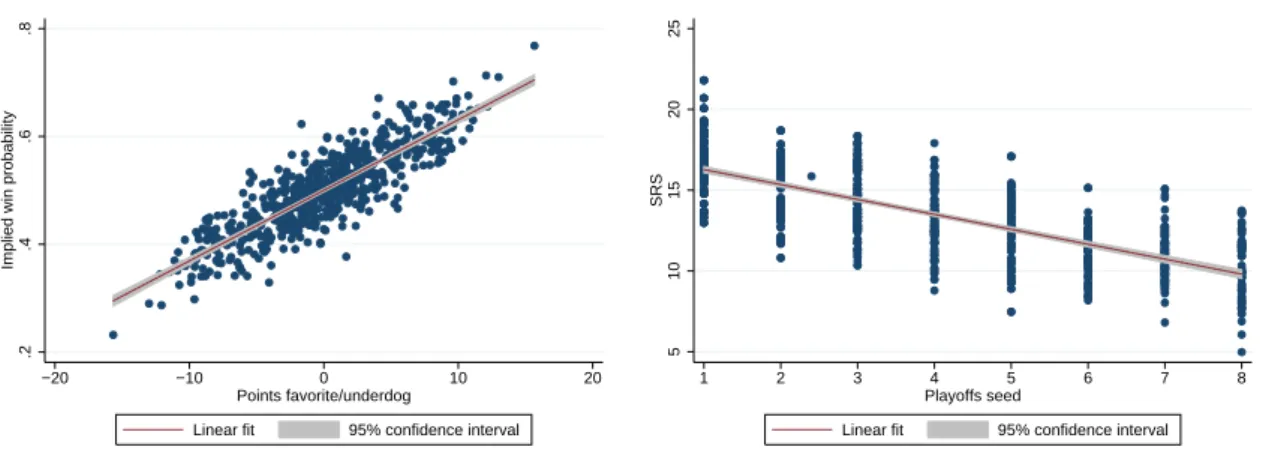
ability measure are highly correlated with betting odds as is illustrated in the left panel of Figure 1.

The SRS-based ability measure is also highly correlated with the ability-based tournament seeds in the playoffs as shown in the right panel of Figure 1. In the empirical analysis we use as a baseline a constant ability indicator, which is exclusively based on information from the regular season preceding the respective elimination tournament, and which is not influenced by the performance during the playoffs.

Figure 1: Validation of the Measure of Ability Using the SRS

.2.4.6.8Implied win probability

−20 −10 0 10 20

Points favorite/underdog

Linear fit 95% confidence interval

510152025SRS

1 2 3 4 5 6 7 8

Playoffs seed

Linear fit 95% confidence interval

Left panel: Implied win probabilities (calculated using the SRS in a Tullock-type probability function) against mean point differentials per matchup, prediction by betting markets for rounds 1-3 in NBA seasons 1991 through 2013. N = 644

Right panel: SRS against tournament seed for rounds 1-3 in NBA seasons 1984 through 2014. N = 868

To compute an empirical measure of heterogeneity (labelled heterogeneity

in the empirical analysis) on a given stage of the tournament that corresponds to θ

in the theoretical model, let a

be the SRS score of a favorite and an underdog team (i = {F,U}), respectively, who compete on stage t. Current heterogeneity on stage t is then computed as

heterogeneity

= a

a

, (8)

where heterogeneity

≥ 1 holds due to the definition of favorite and underdog teams (since a

≥ a

). The advantage of computing the measure of heterogeneity for favorites and underdogs is that the effects of changes in heterogeneity

work in the same direction for both teams. Using instead a symmetric measure of heterogeneity in terms of relative

11We obtained betting odds data fromwww.covers.com.

ability – relating own ability and opponent ability as implied by θ

– would imply that changes in relative ability would have opposite effects on the effort provision of favorites and underdogs. Intuitively, heterogeneity increases if the relative ability of the favorite increases, while heterogeneity decreases if the relative ability of the underdog improves.

This would complicate the empirical analysis and its interpretation unnecessarily. The empirical measure of heterogeneity, heterogeneity

, is thus directly linked to the measure θ

used in the theoretical analysis. The only modification is that this measure implicitly assumes a discriminatory power of r = 1, which corresponds to the classic specification of a Tullock contest technology. As a robustness analysis discussed below, we relax this assumption and estimate r from the data to construct an alternative measure of hetero- geneity along the lines of the theoretical model.

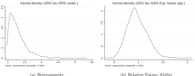
Panel (a) of Figure 2 plots the empirical kernel density of the respective heterogeneity measure and shows that games with comparatively low degrees of heterogeneity are most frequently observed in the data. High degrees of heterogeneity where θ

> 1.5 are rather the exception than the rule.

The empirical measure for relative ability of team i ∈ {F,U} in stage t + 1 of the tour- nament against the opponent team with ability a

– which is labelled E

[rel. ability

] in the following and corresponds to κ

in the theoretical analysis – is constructed in analogy to the index of heterogeneity on the current stage t. In particular, the measure of expected relative ability in future interactions, based on information available at stage t, is constructed as

E

[rel. ability

] = a

E

[a

] . (9)

Importantly, this measure accounts for future relative ability rather than future hetero-

geneity, since the effect of future heterogeneity on the continuation value is different for

teams that are the favorite or the underdog, respectively, in the future interaction. The ex-

pected ability of the opponent on stage t + 1, a

can be constructed in different ways,

depending on the assumptions made on the expectation formation process. For simplicity

and transparency, in the construction of the empirical measures we restrict attention to

competitors on the immediately next stage only. As baseline measure, we consider a con-

vex combination of the ability levels of the two teams in the parallel match-up, the winner

Figure 2: Distribution of Heterogeneity θ and Relative Future Ability κ

0.511.522.5

1 1.5 2 2.5 3 3.5

kernel = epanechnikov, bandwidth = 0.0388

Kernel density (SRS fav./SRS under.)

(a) Heterogeneity

0.511.52

.5 1 1.5 2

kernel = epanechnikov, bandwidth = 0.0333

Kernel density (SRS fav./SRS Exp. future opp.)

(b) Relative Future Ability

Notes: The figures plot kernel densities of the heterogeneity measure and the measure of expected relative ability in the next round, respectively, using the raw data used in the estimation exercises. N = 434

of whom will be the competitor on stage t + 1 of the team under consideration at the current stage t. The ability levels are weighted by the respective winning probabilities.

The reason is that, in many instances, the identity of the future opponent team is not

known yet when decisions are made on the current stage. The structure of the compe-

tition implies, however, that teams competing in stage t know that they will compete

against the winner of the parallel stage-t match on the next stage. Given that abilities of

those teams competing in this parallel match are observable, teams can form expectations

about the probabilities with which they face any one of the two potential opponent teams

in the next stage. In the empirical analysis, we then compute the expected ability of the

opponent i in stage t + 1 as in condition (5). In the robustness section, we also present

the results under different assumptions regarding the expected relative ability on the next

stage. In particular, we consider measures that are based exclusively on the relative ability

of the favorite in the parallel match-up, or adjusted measures that incorporate for each

game if the competitor is already known at the time of the game, and replace the convex

combination by the ability of the actual next competitor. Panel (b) of Figure 2 plots the

empirical kernel density of future relative ability for current favorites.

3.3 Measuring Effort

Whereas one can think of many indicators for final outcomes or performance, constructing a measure of effort of a team or of total effort per game by two teams is not entirely straightforward. In the empirical analysis of this paper, we use the number of personal fouls that a team is called for as a proxy for effort of a team. A personal foul in basketball is defined as a breach of the rules that regulate the legal or illegal form of personal contact between players. This mostly involves attempts to prevent the opposing team from scoring. These fouls are thus called defensive fouls. Much less frequent are offensive fouls that occur during an offensive phase when an illegal scoring attempt is observed.

Hence, both types of fouls measure an attempt to change the course of a game in order to win. Consequently, the number of fouls in a game is a direct indicator for the intensity of the competition and, thus, for the effort of the respective team. In principle, fouls measure how intense the defender attacks his opponent, how physically close he is in coverage, which may sometimes result in a personal foul. Notice that for this to hold it is not necessary to assume that teams explicitly decide to foul their opponent. Rather, it is presumably more likely that players try to avoid fouls in most instances, but are still more likely to foul the opponent when defending intensively. In that sense, personal fouls are an almost natural outcome of an intense game with close physical contact. The higher the intensity, the higher the probability that a foul is inadvertently committed and called.

The intensity of play by a particular team, hence, should be highly correlated with the effort provided.

This measure corresponds closely to a measure of team effort since personal fouls can

be committed by all players of a team. The number of personal fouls is mostly influenced

by a team’s own effort, and a good proxy for how much effort is put on defending the

opponent. More personal fouls correspond to a more physical, thus more tiring, style of

play. Finally, one might be worried that there are different reasons to commit a foul than

an intensive defense, such as intentional fouls for tactical reasons. One situation where

intentional fouling might be an optimal strategy for a team is when the members of the

team get tired and are not able anymore to defend without committing a foul. However,

even if fouls are committed by mistake, or tactically, because players are worn out, this

provides a useful indicator of the physical intensity of the match for a given team as

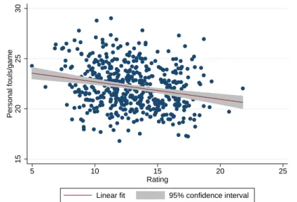
Figure 3: Personal Fouls per Game in Regular Season vs. Ability Measure (SRS)

15202530Personal fouls/game

5 10 15 20 25

Rating

Linear fit 95% confidence interval

Notes: Average number of personal fouls per game in regular season against SRS.N = 496

fatigue is a clear indicator that the intensity – and therefore effort – has been on a high level during the game. Fouling may also be an optimal strategy to stop the clock at the end of a very close game when a team is trailing. While it is neither direct offensive or defensive effort, it is still an attempt to exert every available strategy to win the game, i.e., effort. Consequently, personal fouls appear as the most suitable of the available effort measures for the present paper.

A potential problem with this measure is that the number of personal fouls a team

is called for might be affected by the ability of a team in a counterintuitive manner when

thinking about effort. In particular, the theoretical model predicts that effort is increasing

in ability, while it seems more reasonable to expect that more able teams are also more

able to avoid fouls when defending intensively. This is also what we observe in the long-

term regular season data, the pairwise correlation coefficient associated with the numbers

shown in Figure (3) is -0.22 and highly significant. To control for a team’s ability to

avoid fouls as well as for the style of play of a particular team – the defense of some

teams might explicitly decide to foul more often independent of the opponent team – our

preferred proxy for team effort is the number of fouls per game relative to the average

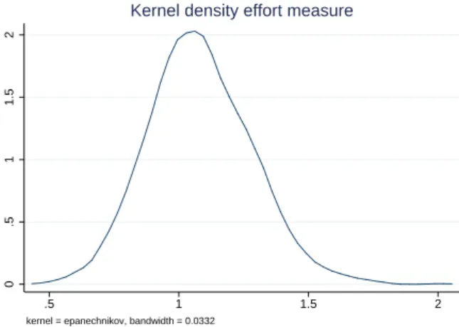
Figure 4: Distribution of Effort Measure

0.511.52

.5 1 1.5 2

kernel = epanechnikov, bandwidth = 0.0332

Kernel density effort measure

Notes: The figures plot the kernel density of the effort measure, using the raw data used in the estimation exercises. N = 434

per-game number of fouls the team has committed in the regular season preceding the playoffs.

This measure is formally defined as

ef f ort

= number of fouls in playoff game

number of games_k

(10)

for team i in year k in stage t of the tournament. Figure 4 plots the kernel density of this effort measure and shows that teams tend to foul more often in the playoffs than in the regular season on average.

When considering the effort measure in terms of personal fouls conditional on the ability during the playoffs, however, the data reveal no clear systematic relationship.

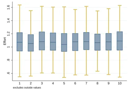
Figure 5 presents a box plot of the effort distribution during the playoffs by ability decile.

There is no systematic relationship, in contrast to what one would expect if effort were misspecified in terms of capturing merely some aspect of ability (or incompetence), where one would expect a systematic relationship between effort and ability throughout the tournament.

Teams are also likely to adjust to the style of play of their opponents, as the system of the opponent’s coach might differ across teams. It is therefore necessary to control for

12Relating the number of fouls per game relative to the average number of fouls during the regular season plays a similar role as season-team fixed effects by accounting for different styles of play, team compositions, coaching styles, etc., in a given season.

Figure 5: Effort Measure vs. Deciles of Ability Rating (SRS)

.6.811.21.41.6Effort

1 2 3 4 5 6 7 8 9 10

excludes outside values

Notes: Effort, as defined in (10) for deciles of ability measured by the SRS for rounds 1–3 for NBA seasons 1984–2014. Outliers are excluded. N = 4398

various indicators describing how opponents usually play the game. The nature of the data allows us to use regular season statistics in order to control for team-specific playing styles. One crucial measure for the likelihood that a foul is called is the style of offense the opponent plays in terms of the distance from which they make their shot attempts.

An increased number of shot attempts from behind the three-point line by the opponent could therefore reduce the number of fouls, independent of effort provided.

In order to account for this, we control for the opponent team’s number of three-point attempts in the regular season. Finally, we also control for the speed of the opponent’s play, as it seems quite possible that a team will commit fewer fouls if the opposing team is slowing down the game in order to reduce certain disadvantages. A good proxy for how fast an opponent plays is the absolute number of field goal attempts per minute, which is used in the form of the regular season average as a control variable.

Another concern for the effort measure could be the presence of a so-called zone de- fense. A zone-defense is a style of defense which is less physical and relies more on optimal positioning in space and, thus, might produce fewer fouls, independent of effort provided.

13The three-point line is a mark on the floor which separates the area where a successful basket counts two points from the rest of a field where it is worth 3 points. The distance between the three- point line and the basket has been the subject of multiple changes since the founding of the NBA. See www.nba.com/analysis/rules_history.html.

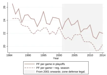
One practical way of operating against an opposing zone defense is to concentrate more on distance shooting. The number of attempted three-point shots should increase in the presence of a zone defense, as these defenses can be better attacked from the distance and are known for leaving three-point shots open. Figure 6 plots the evolution of fouls over time. The change in background shade indicates the rule change in the 2000/01 NBA season, which made zone defense illegal.

The figure suggests that the rule change had no effect on the average number of fouls, and the long time trend remained unaffected. In the empirical analysis we will control for season fixed effects, which should also take care of the time trend in the average number of personal fouls.

Figure 6: Personal Fouls During the Regular Season and During Playoff Tournaments

20222426

1984 1990 1995 2000 2005 2010 2014

Year PF per game in playoffs PF per game−−reg. season

From 2001 onwards: zone defense legal.

A similar approach to use data on fouls as proxy for effort has been used before by Berger and Nieken (2014) as well as by Deutscher, Frick, G¨ urtler, and Prinz (2013) in the context of handball and soccer, respectively. Both studies rely on regular season data, however, which implies that they cannot control for the usual style of play of a team, as is done in the construction of the effort measure by relating effort in a given game to average effort in the regular season. Another difference to their approach is that we do not distinguish between destructive and productive effort, as both should have an

14A zone defense is a form of defense where a player is defending a certain area rather than defending against an opposing player. A detailed overview on the evolution of rules regarding illegal defense is to be found at www.nba.com/analysis/rules_history.html.

identical positive influence on the probability to win.

In light of this, and given the intensity and strictness of rules in basketball, we view fouls as an equally or even more appropriate measure in the context of this paper.

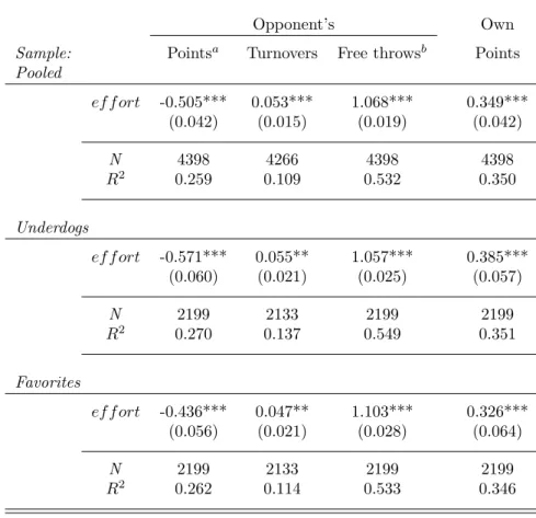
The discussion so far has provided several arguments for the suitability of the number of personal fouls as an effort indicator in the context of this paper. In what follows, we provide more direct evidence on the arguments made so far. Recall that we use fouls as a measure of effort, since fouls measure how intense the defender attacks his opponent and how physically close he is in coverage. This type of defensive effort may then sometimes – but not always – result in a personal foul. We would thus expect that higher defensive effort increases turnovers of the opponent team (i.e. stealing the ball) and thereby helps to prevent the opponent from scoring. Since this implies that intensively defending teams a higher share of ball possession, and since ball possession is necessary to score, we would also expect that intensively defending teams score more often.

Table 1 presents the corresponding regression results that document that higher ef- fort, indeed, increases turnovers of the opponent team, both for underdogs and favorites.

Moreover, effort reduces the points scored by the opponent team out of the field (net of free throws), suggesting that one additional foul (relative to the regular season average) reduces points of the opponent team by 0.50. The effect is slightly larger when considering only the sample of underdogs, and slightly lower when considering favorites, but the dif- ferences are not significant. Finally, more fouls are apparently successful in increasing the number of own points scored, maybe because higher turnover rates make quick advances on offense more profitable. Again, the effect appears to be slightly larger for underdogs than for favorites. The downside of more effort in terms of personal fouls, however, is a higher number of free throws for the opponent team. According to the point estimates, one additional foul leads to one additional point from free throws for the opponent team.

15Lazear (1989) analyses tournament situations where high incentives increase the effort of tournament participants, which is increasing the surplus of the tournament. On the other side, high incentives may also lead to more sabotage behavior, which will, in turn, reduce the surplus. In contrast to such a situation in a firm, defensive actions of a sports team should not be interpreted as sabotage behavior, because they do not reduce the surplus of the match. While, in principle, a surplus in a sports competition is difficult to define, it should be related to the suspense or thrill of the game for the spectators, which will in any case be positively related to the intensity of the game. In a similar vein, Bartling, Brandes, and Schunk (2015) find that teams react by the number of rule breaches, measured by the assignment of cards in soccer.

Table 1: Validation: The Effect of Effort on Outcomes

Opponent’s Own

Sample: Points^a Turnovers Free throws^b Points Pooled

ef f ort -0.505*** 0.053*** 1.068*** 0.349***

(0.042) (0.015) (0.019) (0.042)

N 4398 4266 4398 4398

R² 0.259 0.109 0.532 0.350

Underdogs

ef f ort -0.571*** 0.055** 1.057*** 0.385***

(0.060) (0.021) (0.025) (0.057)

N 2199 2133 2199 2199

R² 0.270 0.137 0.549 0.351

Favorites

ef f ort -0.436*** 0.047** 1.103*** 0.326***

(0.056) (0.021) (0.028) (0.064)

N 2199 2133 2199 2199

R² 0.262 0.114 0.533 0.346

Robust standard errors (clustered for individual playoff-series) in round parentheses. All specifications include a dummy equal to 1 if team plays at home, a a dummy equal to 1 if series is decided in best-of-7 mode with best-of-5 as the base category, playoff-stage dummies, and overtime dummies. *, ** and *** indicate statistical significance at the 10-percent level, 5-percent level, and 1-percent level, respectively.

aTotal number of opponent’s points scored from the field (without points from free throws).

bTotal number of opponent’s free throws taken.

Since many statistics in basketball are influenced by ability and effort choices, one

might consider various other statistics as proxies for effort provision. Goldman and Rao

(2012) analyze effort in regular season NBA games in the context of pressure in home

games, identifying defensive rebounds as defensive and offensive rebounds as offensive

effort. Any rebound in basketball, however, is strongly affected by the efforts of both

teams, rendering it problematic as measure of a given team’s effort. Moreover, rebound

rates by definition add up to one, since the more rebounds one team achieves the lower the

rebound rate of the opponent. Being a share between zero and one, rebound rates cannot

be used as an effort measure, where both teams’ effort is supposed to react.

Another indicator is the number of blocked shots, which has similar deficiencies for the purposes of this paper. An alternative statistic that should be highly correlated with defensive effort, and therefore more closely corresponds to the theoretical conceptualization of effort is the number of steals. Steals are to a lesser degree influenced by both team’s effort, but they are highly influenced by abilities. In sum, the number of personal fouls appears as the measure of effort that is suited best for the purposes of this paper.

3.4 Empirical Framework

In order to test the theoretical predictions about the implications of heterogeneity on the current stage, and of expected relative ability on the next stage, we use a simple reduced form linear estimation framework that allows to test the comparative static predictions of condition (7). In particular, we estimate the empirical model

effort

= β

+ β

heterogeneity

+ β

E

[rel. ability

] + Ω

X + , (11) where heterogeneity

is the empirical counterpart to θ

and rel. ability

is the empirical counterpart to κ

.

The coefficient β

incorporates, among other things, the discrimi- natory power r that is constant across agents and stages, while β

measures the (average) effect of absolute ability on effort. Results 1 and 2 provide directed hypotheses about the expected signs of coefficient estimates β

and β

: First, β

– the effect of current hetero- geneity θ

on stage-t effort – is predicted to be negative. In addition, β

should be higher in absolute terms in the sub-sample of favorites than in the sub-sample of underdogs.

Second, β

– the effect of future relative ability κ

on stage-t effort – is predicted to be positive if agents are forward looking, and zero if agents entirely focus on the immediate

16Goldman and Rao (2012) are interested in the effect of pressure in a home game on effort. In this case, rebound rates are appropriate, but the differential effect of crowd cheering on the home vs. the away team cannot be identified with this measure.

17Estimates for more flexible specification that derives directly from a log-linearized version of (7) with Rnow = 0 deliver qualitatively very similar results. In particular, substituting condition (6) into (7), taking logs and simplifying under the assumption thatr= 1 delivers

lne_t = b₀+b₁(lnθ_t) +b₂(lnκ_t+1) +b₃ln(1 +θ_t) +b₄ln(1 +κ_t+1), (12) with b being parameters to be estimated. Due to the collinearity of the respective terms that includeθ andκ, this specification delivers estimates that are less reliable and more difficult to interpret.

consequences of their actions. When applying this to the data using the measure of effort defined in equation (10), there are two minor issues that need to be noticed. First, the estimation framework does not control for the absolute ability of a team, since the effort measure is normalized with respect to the regular season average, which already accounts for ability.

Second, the empirical specification includes additional controls for the team’s and the opponent’s styles of play. These modifications deliver the following estimation equation. Specifically, the vector X controls for team-specific playing styles such as the opponent’s free throw percentage in the regular season, the opponent’s three-point per- centage, the absolute number of own shot attempts, the opponent’s absolute number of shot attempts, the number of three-point shot attempts allowed and the percentage of suc- cessful three-point shots allowed – everything measured for the regular season preceding the playoffs. Moreover, X includes a variable counting the number of previous meetings in the preceding regular season, a dummy variable equal to 1 if the team i plays at home, a dummy equal to 1 if the series are decided in best-of-7 mode with best-of-5 as the base category, playoff-stage dummies, standings dummies

and overtime dummies.

Note that the unit of observation in the empirical analysis is a single game. The main hypothesis underlying the analysis concerns the impact of the expected strength of the future opponent on current effort: variations in the strength of the future opponent change the incentives of a team from the outset of the game, but not within the game. Hence, we are not interested in (minute-by-minute) dynamics within a game. The dynamics within a game depends on the effort – and success – of the two teams as the game proceeds and can be considered as noise with respect to our main hypothesis.

18Unreported results show that adding ability as an additional control variable delivers coefficient estimates for this variable that are always insignificant, as one would expect if ability is already controlled for by the normalization of the effort measure. Details available from the authors upon request.

19All standings are defined from the perspective of the observed team. A standing of, e.g., ‘1-0’ indicates that the current observation is in the second game with the observed team leading the playoff series by one game.

20We also estimate a specification including the number of rest days and the travel distances between team locations. The results do change neither qualitatively nor quantitatively.

4 Results

4.1 Main Results

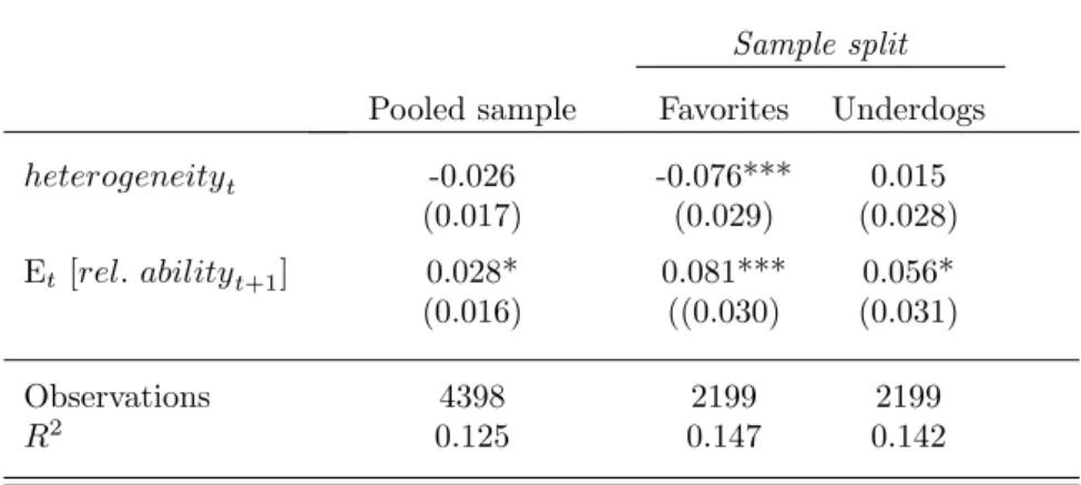
Table 2 presents the main results from estimating model (11). The results reveal that teams indeed adjust their effort in response to the current opponent’s ability: if the ratio of a team’s own rating over the current opponent’s rating increases, teams reduce their effort. Given that favorites and underdogs in a game may have different incentives and possibilities to react to variations in heterogeneity, we also present results for splitting the sample between favorites and underdogs. Regardless of the specification, the negative effect of heterogeneity is more pronounced for favorites than underdogs. These patterns are consistent with the predictions of Result 1. Regarding the key question of this paper about the implications of variations in the expected relative ability on the next stage of the tournament, the results reveal a positive effect on effort in the current round. Thus, teams exert more effort in response to standing a better chance of prevailing on the next stage of the tournament, consistent with the predictions of Result 2. This effect is significant and visible in all specifications. In particular, there are only minor, insignificant differences between favorites and underdogs.

The log-log specification implies a straightforward quantitative interpretation: if cur- rent relative strength is higher by one percent, current effort increases by 3 percent. The shadow of the future is even larger: if the expected future opponent’s relative strength is higher by one percent, current effort is reduced by 5 percent. In terms of relative strength of the effects, the effort effect of future relative ability is typically even larger than the effect of current heterogeneity.

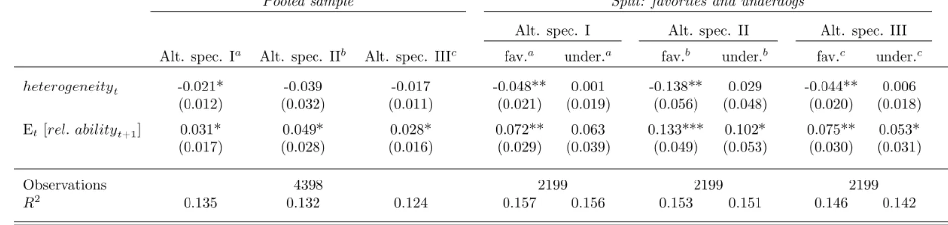
4.2 Robustness and Additional Results

In this subsection, we investigate the robustness of the results as well as additional im-

plications regarding the strength of the effects in different contexts. Table 3 presents the

results from estimating model (11), using three alternative specifications of the measures

of heterogeneity and relative ability on the next stage. Specification (1) uses logged effort

as dependent variable, regressed on heterogeneity measures in terms of logged ratios, as

Table 2: Effect of Current and Future Heterogeneity on Effort

Sample split Pooled sample Favorites Underdogs

heterogeneity_t -0.026 -0.076*** 0.015

(0.017) (0.029) (0.028)

Et[rel. ability_t+1] 0.028* 0.081*** 0.056*

(0.016) ((0.030) (0.031)

Observations 4398 2199 2199

R² 0.125 0.147 0.142

Coefficients for additional variables controlling for team specific characteristics are not reported due to space limitations. All specifications include a dummy equal to 1 if team plays at home, a a dummy equal to 1 if series is decided in best-of-7 mode with best-of-5 as the base category, playoff- stage dummies, standings dummies and overtime dummies. *, ** and *** indicate statistical significance at the 10-percent level, 5-percent level, and 1-percent level, respectively. Robust standard errors (clustered for individual playoff-series) in round parentheses. Dependent variable is defined as log[fouls in playoff game]−log[avg. fouls regular season].

stipulated by a log-linearized approximation to the theoretical condition. Alternatively, Column (2) reports results for a specification where both on the left and the right-hand- side of the equation linear (instead of logged) measures are used. Specification (3) uses a linear specification of heterogeneity in terms of differences rather than ratios. All three specifications deliver a pattern of results that is consistent with the baseline results of Table 2. If anything, the effects are even quantitatively somewhat larger.

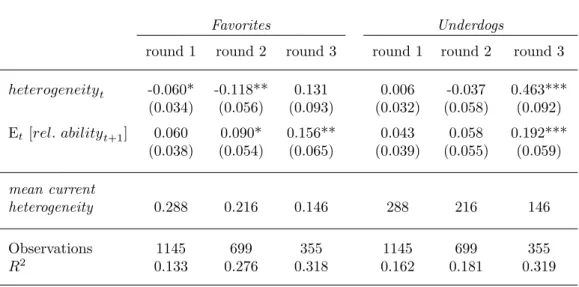
Next, we consider round effects and the importance of the current game for reaching

the next round of the tournament. Intuitively, heterogeneity in the early rounds of the

tournament might have different effects, and take different forms, than in later stages,

such as the semi-final, when the possibility to win the championship is very salient. Ex-

pecting to meet a weak opponent in the next round(s) increases the chances to win the

championship, but more so the fewer rounds are still to go and the less uncertainty is

involved regarding relative future ability. This strategic aspect may be less important

when the finals are still far away. Therefore, in a first set of additional results we estimate

the effects separately at the different stages of the NBA playoff tournament.

Table 3: Effect of Current and Future Heterogeneity on Effort: Alternative Specifications

Pooled sample Split: favorites and underdogs

Alt. spec. I Alt. spec. II Alt. spec. III Alt. spec. I^a Alt. spec. II^b Alt. spec. III^c fav.^a under.^a fav.^b under.^b fav.^c under.^c

heterogeneity_t -0.021* -0.039 -0.017 -0.048** 0.001 -0.138** 0.029 -0.044** 0.006

(0.012) (0.032) (0.011) (0.021) (0.019) (0.056) (0.048) (0.020) (0.018)

Et [rel. ability_t+1] 0.031* 0.049* 0.028* 0.072** 0.063 0.133*** 0.102* 0.075** 0.053*

(0.017) (0.028) (0.016) (0.029) (0.039) (0.049) (0.053) (0.030) (0.031)

Observations 4398 2199 2199 2199

R² 0.135 0.132 0.124 0.157 0.156 0.153 0.151 0.146 0.142

Coefficients for additional variables controlling for team specific characteristics are not reported due to space limitations. All specifications include a dummy equal to 1 if team plays at home, a a dummy equal to 1 if series is decided in best-of-7 mode with best-of-5 as the base category, playoff-stage dummies, standings dummies and overtime dummies. *, ** and *** indicate statistical significance at the 10-percent level, 5-percent level, and 1-percent level, respectively. Robust standard errors (clustered for individual playoff-series) in round parentheses.

aDependent variable is defined as fouls in playoff game

avg. fouls regular season. Heterogeneity_tis defined as ^{SRSF av}

SRSUnd, rel. abiility_t+1is defined asEXP. OP P. SRS^SRS .

bDependent variable is defined as fouls in playoff game−avg. fouls regular season. Heterogeneitytis defined asSRS_{F av}−SRS_{U nd}, rel. abiilityt+1is defined asSRS−EXP. OP P. SRS.

cDependent variable is defined as log[fouls in playoff game]−log[avg. fouls regular season]. Heterogeneity_tis defined as ^{SRSF av}

SRSUnd, rel. abiility_t+1is defined as log[EXP. OP P. SRS^SRS ].

2 7