Competition, Markups, and the Gains from International Trade

IHS Economics Series Working Paper 299

July 2013

Competition, Markups, and the Gains from International Trade

Chris Edmond

Virgiliu Midrigan

Daniel Yi Xu

Impressum Author(s):

Chris Edmond, Virgiliu Midrigan, Daniel Yi Xu Title:

Competition, Markups, and the Gains from International Trade ISSN: Unspecified

2013 Institut für Höhere Studien - Institute for Advanced Studies (IHS) Josefstädter Straße 39, A-1080 Wien

E-Mail: o ce@ihs.ac.atffi Web: ww w .ihs.ac. a t

All IHS Working Papers are available online: http://irihs. ihs. ac.at/view/ihs_series/

This paper is available for download without charge at:

https://irihs.ihs.ac.at/id/eprint/2211/

Competition, Markups, and the Gains from International Trade

Chris Edmond, Virgiliu Midrigan, Daniel Yi Xu

299

Reihe Ökonomie

Economics Series

299 Reihe Ökonomie Economics Series

Competition, Markups, and the Gains from International Trade

Chris Edmond, Virgiliu Midrigan, Daniel Yi Xu July 2013

Institut für Höhere Studien (IHS), Wien

Institute for Advanced Studies, Vienna

Contact:

Chris Edmond

Department of Economics University of Melbourne Parkville VIC 3010, Australia email: cedmond@unimelb.edu.au Virgiliu Midrigan

Federal Reserve Bank of Minneapolis 90 Hennepin Avenue

Minneapolis, MN 55401, USA email: virgiliu.midrigan@nyu.edu and NBER

Daniel Yi Xu

Department of Economics Duke University

220 Social Sciences Building Durham, NC 27708-0097, USA Phone: (919) 660-1824 email: daniel.xu@duke.edu and NBER

Founded in 1963 by two prominent Austrians living in exile – the sociologist Paul F. Lazarsfeld and the economist Oskar Morgenstern – with the financial support from the Ford Foundation, the Austrian Federal Ministry of Education and the City of Vienna, the Institute for Advanced Studies (IHS) is the first institution for postgraduate education and research in economics and the social sciences in Austria. The Economics Series presents research done at the Department of Economics and Finance and aims to share “work in progress” in a timely way before formal publication. As usual, authors bear full responsibility for the content of their contributions.

Das Institut für Höhere Studien (IHS) wurde im Jahr 1963 von zwei prominenten Exilösterreichern – dem Soziologen Paul F. Lazarsfeld und dem Ökonomen Oskar Morgenstern – mit Hilfe der Ford- Stiftung, des Österreichischen Bundesministeriums für Unterricht und der Stadt Wien gegründet und ist somit die erste nachuniversitäre Lehr- und Forschungsstätte für die Sozial- und Wirtschafts- wissenschaften in Österreich. Die Reihe Ökonomie bietet Einblick in die Forschungsarbeit der Abteilung für Ökonomie und Finanzwirtschaft und verfolgt das Ziel, abteilungsinterne Diskussionsbeiträge einer breiteren fachinternen Öffentlichkeit zugänglich zu machen. Die inhaltliche Verantwortung für die veröffentlichten Beiträge liegt bei den Autoren und Autorinnen.

Abstract

We study the gains from trade in a model with endogenously variable markups. We show that the pro-competitive gains from trade are large if the economy is characterized by (i) extensive misallocation, i.e., large inefficiencies associated with markups, and (ii) a weak pattern of cross-country comparative advantage in individual sectors. We find strong evidence for both of these ingredients using producer-level data for Taiwanese manufacturing establishments. Parameterizations of the model consistent with this data thus predict large pro-competitive gains from trade, much larger than those in standard Ricardian models. In stark contrast to standard Ricardian models, data on changes in trade volume are not sufficient for determining the gains from trade.

Keywords

Productivity, misallocation, comparative advantage, intra-industry trade

JEL Classification

F1, O4

Comments

We thank Fernando Alvarez, Costas Arkolakis, Ariel Burstein, Vasco Carvalho, Andrew Cassey, Arnaud Costinot, Jan De Loecker, Ana Cecilia Fieler, Phil McCalman, Markus Poschke, Andrés Rodrίguez- Clare, Barbara Spencer, Iván Werning, and seminar participants at UBC, UC Berkeley, Chicago Booth, Deakin, Harvard, MIT, Monash, UNSW, NYU Stern, Princeton, Stanford, Vanderbilt, the 2011 SED annual meeting, NBER Macroeconomics and Productivity meeting, Melbourne Trade Workshop, FRB Philadelphia International Trade Workshop, and the 2012 FIU International Trade Workshop, Barcelona Industry and Labor Market Dynamics Workshop and CIREQ Macroeconomics Conference. We also thank Jiwoon Kim and Fernando Leibovici for their excellent research assistance.

Contents

1 Introduction 1

2 Model 4

2.1 Consumers and final good producers ... 4

2.2 Intermediate inputs ... 5

2.3 Equilibrium ... 10

2.4 Aggregation ... 10

3 Data 13

3.1 Measurement ... 13

3.2 Key facts ... 14

4 Quantifying the model 16

4.1 Overview ... 16

4.2 Productivity distribution ... 16

4.3 Calibration ... 18

5 Gains from trade 22

5.1 Efficiency losses due to misallocation ... 22

5.1.1 Economy with Taiwan's import share ... 22

5.1.2 Economy under autarky ... 23

5.2 Welfare gains. Identical Home and Foreign productivity ... 23

5.3 Welfare gains. Independent Home and Foreign productivity ... 25

6 General model 26

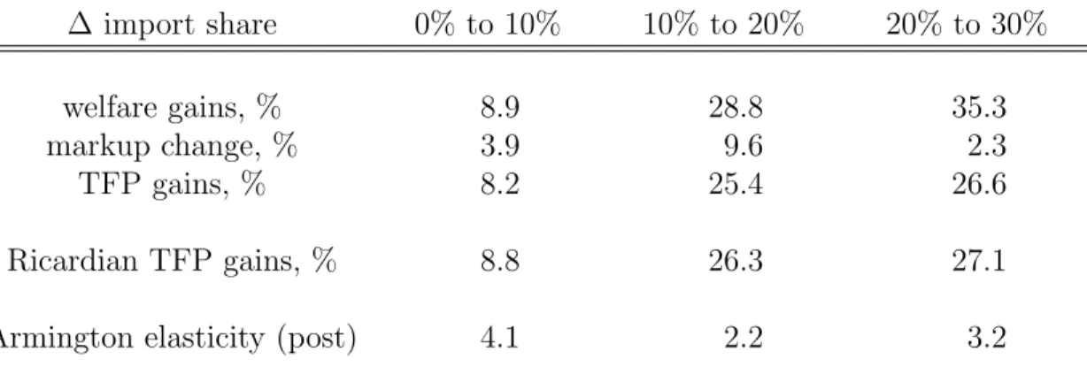
6.1 An increase in the import share from 0 to 10% ... 26

6.2 An increase in the import share from 10 to 20% ... 27

6.3 Evidence on the amount of dependence ... 27

7 Comparison with standard trade models 28

7.1 Comparison with the ACR approach ... 29

7.2 Comparison with calibrated standard model ... 30

8 Robustness experiments 30 9 Evidence for the pro-competitive mechanism 32

9.1 Taiwanese manufacturing ... 33

9.2 US manufacturing ... 33

10 Conclusions 35

References 35

Tables 38

Figures 45

1 Introduction

How large are the welfare gains from international trade? We answer this question using a quantitative model with endogenously variable markups. In such a model, trade can increase productivity and welfare via two channels. First, if opening an economy to trade exposes domestic firms to more competition, then there may be gains due to reduced markups and reduced markup dispersion. We refer to these as pro-competitive effects. Second, as in standard models, opening to trade implies welfare and productivity gains due to Ricardian effects. Our goal is to measure the strength of these two effects using producer-level data.

One of the oldest ideas in economics is that opening an economy to trade may lead to welfare gains from increased competition. And existing empirical work provides support for this idea.

¹

But, perhaps surprisingly, existing trade models with variable markups do not generally predict pro-competitive effects. Indeed, the workhorse trade model with variable markups studied by Bernard, Eaton, Jensen and Kortum (2003, hereafter BEJK) implies exactly zero pro-competitive gains from trade, as does the model of Arkolakis, Costinot and Rodr´ıguez-Clare (2010). Moreover, recent work by Arkolakis, Costinot, Donaldson and Rodr´ıguez-Clare (2012b) shows that pro-competitive effects can be negative.

We study the gains from trade in the model developed by Atkeson and Burstein (2008).

In this model, any given sector has a small number of producers who engage in oligopolistic competition. The demand elasticity for any given producer, and hence its markup, depends on the producer’s sectoral sales share. A reduction in trade barriers reduces the sectoral share of domestic producers, thus reducing their markups.

We focus on the Atkeson and Burstein (2008) model for a number of reasons. First, the model is a parsimonious extension of the BEJK model, widely used in existing work. Unlike in BEJK, however, the markup distribution in the Atkeson and Burstein (2008) model may vary over time and in response to changes in trade policy. Moreover, the model nests BEJK as a special case and is sufficiently rich to produce a wide range of implications regarding the size of the pro-competitive gains from trade. Finally, because the model implies a direct link between individual markups and a producer’s sectoral sales share, the model can be straightforwardly parameterized using micro data on sectoral shares.

We show that the pro-competitive gains from trade in the Atkeson-Burstein model can be

1We discuss evidence for pro-competitive effects, including a brief survey of existing work, in Section 9 below. By contrast, see De Loecker, Goldberg, Khandelwal and Pavcnik (2012) for evidence that markups increaseafter a trade liberalization.

large, much larger than those implied by standard trade models,

²

so long as two conditions are satisfied. First, there must be large inefficiencies associated with markups to begin with, i.e., there must be extensive initial misallocation. Second, the pattern of cross-country comparative advantage in individual sectors must be relatively weak, i.e., trade partners must be characterized by relatively similar productivities within a given sector.

The first condition is obvious and intuitive. There simply cannot be large pro-competitive gains from trade if there are only small distortions associated with markups to begin with.

The second condition is also intuitive. Trade can only reduce markups if it in fact increases the amount of competition faced by domestic producers in individual sectors. If trade partners are characterized by similar productivities within a given sector, then opening to trade exposes domestic producers to more intense head-to-head competition and forces them to reduce markups. By contrast, if there are large cross-country differences in sectoral productivity, then the pro-competitive gains from trade are small or even negative. In this latter case, most of the increase in trade is on the extensive margin: a country that opens up to trade starts importing goods in new sectors, but trade has little effect on the amount of competition faced by domestic producers in existing sectors.

To quantify the model we use product-level (7-digit) Taiwanese manufacturing data. We use the data to discipline two key factors governing the extent of initial misallocation: (i) the elasticity of substitution across sectors, and (ii) the equilibrium distribution of producer- level sectoral shares. The elasticity of substitution across sectors plays a key role because it determines the extent to which producers that face little competition in their own sector can raise markups. We pin down this elasticity by requiring that our model fits the cross- sectional relationship between measures of markups and sectoral shares that we observe in the Taiwanese data. We pin down the parameters governing the producer-level productivity distribution and fixed costs of operating and exporting by requiring that our model reproduces the distribution of sectoral shares and concentration statistics in the Taiwanese data.

The Taiwanese data feature a large amount of dispersion and concentration in producer- level sectoral shares, as well as a very strong relationship between sectoral shares and markups. Interpreted through the lens of the model, this implies a great deal of misallo- cation, due to a high level and dispersion of markups.

Given this initial misallocation, our model predicts large pro-competitive gains from trade

2Eaton and Kortum(2002) andMelitz(2003). See alsoArkolakis, Costinot and Rodr´ıguez-Clare(2012a), who study the welfare gains from trade in this broad class of trade models.

if, in addition, there is a relatively weak pattern of comparative advantage so that increased trade in fact confronts producers with increased competition. To measure the pattern of comparative advantage across Taiwan and its trading partners, we observe that the degree of dispersion in productivity across countries is strongly related to the pattern of intra-industry trade implied by the model. If the pattern of comparative advantage is weak, productivity is relatively similar within a given sector and most trade is primarily intra-industry. If the pattern of comparative advantage is strong, however, so that domestic firms are highly- productive in some sectors while foreign firms are highly-productive in an entirely different set of sectors, then most trade is across industries.

We measure the amount of intra-industry trade using measures of dispersion in sectoral import shares and find that most Taiwanese trade is intra-industry (as is most US trade).

Interpreted through the model, this implies a weak pattern of comparative advantage and hence implies that most of the gains from trade are indeed due to pro-competitive effects.

Our work is related to a number of recent papers. Arkolakis, Costinot and Rodr´ıguez- Clare (2012a) show that the welfare gains from trade are identical in a large class of trade models.

³

These models differ in their micro details, but their aggregate welfare implications are solely determined by the effect a reduction in trade barriers has on the volume of trade.

In our model with variable markups, this aggregation result no longer holds. Even in versions of our model in which Ricardian effects dominate and markups move little in response to changes in trade barriers, data on trade volumes alone are no longer sufficient for determining the welfare gains from trade.

Several recent theoretical papers highlight the connection between endogenously variable markups and the gains from trade.

⁴

In particular, an important recent contribution by De Blas and Russ (2010) extends BEJK to allow for a finite number of producers in a given sector. In their model, as in Atkeson and Burstein (2008), the distribution of markups varies in response to changes in trade costs. Holmes, Hsu and Lee (2011) study that model’s implications for the impact of trade on productivity and misallocation. Relative to these theoretical papers, as well as to earlier studies by Devereux and Lee (2001) and Melitz and Ottaviano (2008), our main contribution is to quantify the pro-competitive mechanism using micro data. In addition, we relax the assumption, commonly made in this literature, that

3These include the models of Armington (1969), Krugman (1980), Eaton and Kortum (2002), Melitz (2003), andBernard et al.(2003).

4See alsoEpifani and Gancia (2011) who consider a trade model with exogenous markup dispersion and Peters(2011) who considers a model with endogenously variable markups but in a closed economy setting.

productivity draws are independent across countries. As discussed above, the pro-competitive effects in our model depend crucially on the extent to which productivities within a given sector are correlated across countries.

Increasing total factor productivity (TFP) by reducing markup dispersion is an effect familiar from the work on misallocation of factors of production by Restuccia and Rogerson (2008), Hsieh and Klenow (2009) and others. We find that international trade can play a powerful role in reducing misallocation and increasing productivity. From a policy viewpoint, our model suggests that obtaining large welfare gains from an improved allocation may not require the detailed, perhaps impractical, scheme of subsidies and taxes that implement the first-best. Instead, simply opening an economy to trade may provide an excellent practical alternative that substantially improves welfare.

We conclude our analysis by presenting evidence of pro-competitive effects. Versions of our model that imply strong pro-competitive effects predict that sectors with higher import shares face more competition from abroad and thus have lower levels and dispersion of markups.

We find strong evidence of these pro-competitive effects in Taiwanese and US data.

The remainder of the paper proceeds as follows. Section 2 presents the model. Section 3 gives an overview of the data, and Section 4 explains how we use that data to quantify the model. Section 5 studies the welfare gains from trade for two extreme parameterizations of the pattern of comparative advantage while Section 6 studies the gains from trade more generally. Section 7 compares the welfare gains in our model to those implied by standard Ricardian models. Section 8 conducts a number of robustness checks. Section 9 provides evidence of strong pro-competitive effects in Taiwanese and US data. Section 10 concludes.

2 Model

The world consists of two symmetric countries, Home and Foreign. We focus on describing the problem of Home agents in detail. We indicate Foreign variables with an asterisk.

2.1 Consumers and final good producers

Each country is inhabited by a continuum of identical consumers. Perfectly competitive firms in each country produce a homogeneous final good that is used for consumption and investment. Final good firms produce using inputs derived from a continuum of sectors.

Importantly, each sector consists of a finite number of domestic and foreign intermediate

goods producers.

Consumers. The problem of Home consumers is to choose aggregate consumption

Ct

, labor supply

Lt

, and investment

Xt

in physical capital to maximize

∞

X

t=0

β^tU

(C

_t, L_t

) subject to

Pt

(C

t

+

Xt

)

≤WtLt

+ Π

t−Tt

+

RtKt,

where

P_t

is the price of the final good,

W_t

is the wage rate, Π

_t

is firm profits,

T_t

is lump-sum net taxes, and

R_t

is the rental rate of physical capital

K_t

, which satisfies

K_t+1

= (1

−δ)K_t

+

X_t.

We assume identical initial capital stocks and technologies in the two countries and that trade is balanced in each period.

Final good producers. The producers of the final good are perfectly competitive. The technology with which they operate is

Y_t

=

Z 1

0

y

θ−1 θ

j,t dj θ−1^θ

,

where

θ >

1 is the elasticity of substitution across sectors

j ∈

[0, 1] and where sectoral output is produced using

N

domestic and

N

imported intermediate inputs,

y_j,t

= 1

N

N

X

i=1

y_ij,t^{H γ−1}_γ

+ 1

N

N

X

i=1

y^F_ij,t^γ−1_γ

!_γ−1^γ

,

(1)

where

γ > θ

is the elasticity of substitution across goods

i

within a particular sector

j

.

2.2 Intermediate inputs

Intermediate goods producer

i

in sector

j

uses the technology

y_ij,t

=

a_ijk^α_ij,tl_ij,t^1−α,

where

a_ij

is the producer’s idiosyncratic productivity (which for simplicity we assume is time-

invariant ),

k_ij,t

is the amount of capital hired by the producer, and

l_ij,t

is the amount of labor

hired. We discuss the assumptions we make on the distribution of firm-level productivity in

Section 4 below. To conserve notation, for the remainder of the paper we suppress time

subscripts whenever there is no possibility of confusion.

Trade costs. An intermediate goods producer sells output to final goods producers located in both countries. Let

y^H_ij

be the amount sold to Home final goods producers, and similarly let

y^∗H_ij

be the amount sold to Foreign final goods producers. The resource constraint for Home intermediates is

y_ij

=

y^H_ij

+ (1 +

τ

)y

_ij^∗H,

where

τ >

0 is an iceberg trade cost, i.e., (1+

τ

)y

_ij^∗H

must be shipped for

y^∗H_ij

to arrive abroad.

We describe an intermediate producer’s problem below, after describing the demand for their good. Due to fixed costs, intermediate producers may decide not to operate. Let the indicator function

φ^H_ij ∈ {0,

1} denote the decision to operate or not in the Home market, and let

φ^∗H_ij ∈ {0,

1} denote the decision to operate or not in the Foreign market.

Foreign intermediate goods producers face an identical problem. We let

y^∗_ij

denote their output and note that the resource constraint for Foreign intermediates is

y_ij^∗

= (1 +

τ)y^F_ij

+

y_ij^∗F,

where

y_ij^∗F

is the amount sold by Foreign intermediates to Foreign final goods producers and

y_ij^F

is the amount shipped to Home final goods producers.

Demand for intermediate inputs. Final good producers buy intermediate goods from Home producers at prices

p^H_ij

and from Foreign producers at prices

p^F_ij

. Consumers buy the final good at price

P

. The problem of a final good producer is to choose intermediate inputs

y_ij^H

and

y_ij^F

to maximize profits:

P Y − Z 1

0

1

N

N

X

i=1

p^H_ijy_ij^H

+ (1 +

τ)

1

N

N

X

i=1

p^F_ijy_ij^F

! dj.

The solution to this problem gives the demand functions

y_ij^H

=

p^H_ij

p_j

!^−γ p_j

P −θ

Y,

(2)

and

y_ij^F

= (1 +

τ

)

p^F_ij pj

!−γ

p_j P

−θ

Y,

(3)

where the aggregate and sectoral price indexes are

P

=

Z 1

0

p^1−θ_j dj 1−θ¹

,

(4)

and

pj

= 1

N

N

X

i=1

φ^H_ij p^H_ij^1−γ

+ (1 +

τ

)

^1−γ

1

N

N

X

i=1

φ^F_ij p^F_ij^1−γ

!1−γ¹

.

(5)

Market structure. An intermediate good producer faces the demand system given by (2)- (5) and engages in Cournot competition within its sector.

⁵

That is, each individual producer chooses a given quantity

y^H_ij

or

y^∗H_ij

, taking as given the quantity decisions of its competitors in sector

j

. Due to constant returns, the problem of a firm in its domestic market and its export market can be considered separately.

Fixed costs. A fixed cost

Fd

, denominated in units of labor, must be paid in order to operate in the domestic market, and a fixed cost

F_f

must be paid in order to export. The firm may choose to produce zero units of output for the domestic market to avoid paying the fixed cost

F_d

. Similarly, the firm may choose to produce zero units of output for the export market to avoid paying the fixed cost

F_f

.

Domestic market. The problem of a Home firm in its domestic market is given by:

π_ij^H ≡

max

y^H_ij,k^H_ij,l^H_ij,φ^H_ij

p^H_ijy^H_ij −Rk_ij^H −W l^H_ij −W F_d φ^H_ij.

Conditional on selling,

φ^H_ij

= 1, the demand for labor and capital satisfy

αvij

y^H_ij

k_ij^H

=

R,

(6)

(1

−α)v_ijy_ij^H

l_ij^H

=

W,

(7)

where

v_ij

is the intermediate’s marginal cost (which, by symmetry, is common to both the domestic and the export market), and is given by:

v_ij

=

V

a_ij,

where

V ≡α^−α

(1

−α)^−(1−α)R^αW^1−α.

(8) Using this notation, we can rewrite the profits of the intermediate producer as

π_ij^H

= max

y^H_ij,φ^H_ij

p^H_ij −v_ij

y^H_ij −W F_d φ^H_ij,

5InSection 8below we solve our model under the alternative assumption ofBertrand competition.

subject to the demand system above. The solution to this problem is characterized by a price that is a markup over marginal cost:

p^H_ij

=

ε^H_ij

ε^H_ij −

1

v_ij.

(9)

Here

ε^H_ij

is the demand elasticity in the domestic market, which satisfies

ε^H_ij

=

ω_ij^H

1

θ

+ 1

−ω_ij^H

1

γ

⁻¹

,

(10)

where

ω_ij^H

is the sectoral share in the domestic market:

ω^H_ij

=

p^H_ijy_ij^H PN

i=1p^H_ijy^H_ij

+ (1 +

τ

)

PN

i=1p^F_ijy_ij^F

= 1

N

p^H_ij p_j

!^1−γ

.

(11)

Sectoral shares and demand elasticity. The demand elasticity faced by any producer is endogenous and given by a weighted harmonic average of the across-sector elasticity

θ

and the within-sector elasticity

γ > θ. Firms with a large share of a sector’s revenue face a lower

demand elasticity and charge a higher markup. These firms compete more with producers in other sectors and so face a demand elasticity closer to

θ. Similarly, firms with a low share

in any individual sector compete mostly with producers in that particular sector and face a demand elasticity closer to

γ. Clearly, the extent of markup dispersion across firms depends

both on the degree of dispersion in sectoral shares within sectors and on the size of the gap between

γ

and

θ. Ifγ

and

θ

are equal, the demand elasticity is constant as in a standard trade model. Alternatively, if

γ

is substantially larger than

θ, then a modest change in sectoral

shares can have a large effect on the demand elasticity.

Sectoral shares and labor shares. The model implies a negative linear relationship between a firm’s sectoral share and its labor share. To see this, observe from (7) and (9) that a firm’s revenue productivity is proportional to its markup:

p^H_ijy_ij^H

W l^H_ij

= 1 1

−α

ε^H_ij

ε^H_ij −

1

.

(12)

Now using (10) to substitute out the elasticity

ε^H_ij

in terms of the sectoral share

ω^H_ij

gives:

W l_ij^H

p^H_ijy^H_ij

= (1

−α)

1

−

1

γ

−

(1

−α)

1

θ −

1

γ

ω_ij^H.

(13)

Since

γ > θ, the coefficient on the sectoral share ω^H_ij

is negative. Section 4 below uses the

linear relationship in equation (13) and micro data on sectoral shares and labor shares to

identify these key elasticity parameters.

Export market and tariffs. The problem of a Home firm in its export market is essentially identical except that (i) to export, it pays a fixed cost

F_f

rather than

F_d

, and (ii) the sales of their good abroad are subject to an ad valorem tariff

ξ∈

[0, 1]. This problem can be written

π^∗H_ij

= max

y^∗H_ij ,φ^∗H_ij

(1

−ξ)p^∗H_ij −v_ij

y_ij^∗H −W F_f φ^∗H_ij ,

subject to the demand system in the Foreign market, analogous to (2) above. We assume that the revenue from tariffs is redistributed lump-sum to consumers in the importing country.

Prices are then given by

p^∗H_ij

= 1 1

−ξ

ε^∗H_ij ε^∗H_ij −

1

v_ij,

where

ε^∗H_ij

is the demand elasticity in the export market:

ε^∗H_ij

=

ω^∗H_ij

1

θ

+ 1

−ω^∗H_ij

1

γ

⁻¹

,

(14)

and where

ω_ij^∗H

is the sectoral share in the export market:

ω_ij^∗H

= (1 +

τ

)p

^∗H_ij y^∗H_ij PN

i=1p^∗F_ij y_ij^∗F

+ (1 +

τ)PN

i=1p^∗H_ij y_ij^∗H.

(15)

Entry and exit. Each period a Home firm must pay a fixed cost

F_d

to sell in its domestic market. The firm sells in the domestic market as long as

(p

^H_ij −v_ij

)y

^H_ij ≥W F_d.

Similarly, the Home firm must pay another fixed cost

F_f

to operate in its export market.

The firm exports as long as

((1

−ξ)p^∗H_ij −v_ij

)y

^∗H_ij ≥W F_f.

There are multiple equilibria in any given sector. Different combinations of intermediate firms may choose to operate, given that the others do not. As Atkeson and Burstein (2008) do, we place intermediate firms in the order of their productivity

a_ij

and focus on equilibria in which firms sequentially decide on whether to operate or not: the most productive decides first (given that no other firm enters), the second most productive decides second (given that no other less productive firm enters), etc.

⁶

6The exact ordering we choose makes little difference quantitatively when we calibrate the model to match the strong concentration in the data. Productive producers always enter and unproductive ones always stay out; the multiplicity of equilibria only affects the entry decisions of small marginal producers that have a negligible effect on the aggregates. Moreover, as we show in Section 8 below, our model’s implications for the gains from trade are essentially unchanged when we set Fd=Ff = 0 so that all producers enter and the equilibrium is unique.

2.3 Equilibrium

In equilibrium, consumers and firms optimize and the markets for labor and physical capital clear:

L_t

=

Z 1

0

1

N

N

X

i=1

l^H_ij,t

+

F_d

φ^H_ij,t

+

l^∗H_ij,t

+

F_f φ^∗H_ij,t

dj

K_t−1

=

Z 1

0

1

N

N

X

i=1

k^H_ij,tφ^H_ij,t

+

k_ij,t^∗Hφ^∗H_ij,t dj.

The market clearing condition for the final good in each country is:

Y_t

=

C_t

+

X_t.

2.4 Aggregation

The model aggregates to a two-country representative agent economy, which is standard ex- cept that TFP, the aggregate markup, and the Armington elasticity are all endogenous. Each of these key objects is determined by underlying productivity differences

aij

, the elasticity of substitution parameters

θ

and

γ, as well as the trade cost and tariff parameters τ, ξ

that govern the amount of trade.

Aggregate productivity. The quantity of final output in each economy can be written

Y

=

AK^αL

˜

^1−α,

where

A

is the endogenous level of TFP,

K

is the aggregate stock of physical capital, and ˜

L

is the aggregate amount of labor used net of fixed costs. Using the firms’ optimality conditions for input choices and the market clearing conditions for capital and labor, it is straightforward to show that aggregate productivity is a quantity-weighted harmonic mean of producer-level productivities:

A

=

Z 1

0

1

N

N

X

i=1

1

a_ij

y^H_ij

Y dj

+ (1 +

τ) Z 1

0

1

N

N

X

i=1

1

a_ij

y_ij^∗H Y dj

!⁻¹

.

(16)

Aggregate markup. Define the aggregate (economy-wide) markup by

M ≡ P

V /A,

that is, aggregate price divided by aggregate marginal cost. Using the firms’ optimality conditions and the market clearing condition for labor, we can write:

WL

˜

P Y

= (1

−α)

1

M.

The aggregate labor share is reduced in proportion to the aggregate markup. Once again, it is straightforward to show that

M

=

Z 1

0

1

N

N

X

i=1

1

m^H_ij

p^H_ijy^H_ij

P Y dj

+ (1 +

τ

)

Z 1

0

1

N

N

X

i=1

(1

−ξ) m^∗H_ij

p^∗H_ij y_ij^∗H P Y dj

!⁻¹

.

(17) That is, the aggregate markup is a revenue-weighted harmonic mean of firm-level markups.

Observe that revenues from abroad are reduced in proportion to the tariff rate

ξ.

Two sources of distortions due to markups. The presence of market power provides two channels that distort equilibrium allocations relative to the efficient level. First, the level of the aggregate markup distorts aggregate labor and investment decisions. From the first-order conditions for the consumers’ problem and the expressions for labor and capital demand, we have

−Ul,t

U_c,t

=

Wt

P_t

= 1

M_t

(1

−α)Yt

L

˜

_t,

and

Uc,t

=

βUc,t+1

R_t+1

P_t+1

+ (1

−δ)

=

βUc,t+1

1

M_t+1αY_t+1

K_t+1

+ (1

−δ)

.

High aggregate markups thus act like distortionary labor and capital income taxes and reduce output relative to its efficient level.

Second, dispersion in markups also reduces the level of aggregate TFP, as in the work of Restuccia and Rogerson (2008) and Hsieh and Klenow (2009). To understand this second effect, notice that the expression for aggregate productivity reduces to

A

=

Z 1

0

mj

M ^−θ

a^θ−1_j dj _θ−1¹

,

where

m_j

=

p_j/(V /a_j

) is the sector-level markup and where sector-level productivity,

a_j

, is

a_j

= 1

N

N

X

i=1

φ^H_ij m^H_ij m_j

!−γ

a^γ−1_ij

+ (1 +

τ

)

^1−γ

1

N

N

X

i=1

φ^F_ij m^F_ij

(1

−ξ)m_j

!−γ

a^∗γ−1_ij

!

1 γ−1

.

The first-best TFP level (attainable by a planner given a particular tariff

ξ) is equal to:

A

=

Z 1

0

a^θ−1_j dj _θ−1¹

,

(18)

where

a_j

= 1

N

N

X

i=1

φ^H_ija^γ−1_ij

+ (1 +

τ)^1−γ

1

N

N

X

i=1

1 1

−ξ

−γ

φ^F_ija^∗γ−1_ij

!_γ−1¹

.

(19)

Absent markup dispersion, TFP is at its first-best level. With markup dispersion, the most productive producers employ a smaller share of the economy’s capital and labor than effi- ciency dictates, since markups and productivity are positively related. Markup dispersion thus lowers TFP by inducing a suboptimal allocation of capital and labor across producers.

Armington elasticity. The Armington elasticity is a key statistic governing the gains from trade in standard trade models. In those models, a high Armington elasticity, of the size inferred from micro trade data, implies small gains from trade since Home and Foreign goods are closely substitutable. We show below that with endogenously varying markups, the gains from trade can be large despite a high Armington elasticity. Here we briefly describe how we compute the Armington elasticity in our model.

The Armington elasticity is defined as the partial elasticity of trade flows to changes in trade costs, and in particular,

1

−σ

=

−∂

log

^1−λ_λ

∂τ ,

where

λ

is the share of spending on domestically produced goods. In our model

λ

is equal to

λ

=

R1 0

PN

i=1p^H_ijy_ij^Hdj R1

0

PN

i=1p^H_ijy_ij^H

+ (1 +

τ)PN

i=1p^F_ijy_ij^F dj

=

Z 1

0

λ_js_jdj,

where

λ_j

denotes the sector-level share of spending on domestically produced goods and where

sj ≡

(p

j/P

)

^1−θ

is each sector’s share in total spending.

Some algebra shows that the Armington elasticity is related to the two key underlying elasticity of substitution parameters

γ

and

θ, according to the weighted average

σ

=

γ Z 1

0

s_jλ_j λ

1

−λ_j

1

−λ dj

+

θ

1

−

Z 1

0

s_jλ_j λ

1

−λ_j

1

−λ dj

.

(20)

To understand this expression, note that a reduction in trade costs changes the aggregate

import share through two channels: (i) by increasing the import shares in each sector

j, an

effect governed by the within-sector elasticity

γ, and (ii) by reallocating expenditure toward

sectors with lower import shares, an effect governed by the between-sector elasticity

θ. The

weight on the within-sector elasticity

γ

is a measure of the dispersion in sectoral import shares. For example, if all sectors have identical import shares,

λ_j

=

λ

for all

j, then changes

in trade costs imply no between-industry reallocation of resources and

σ

=

γ. At the other

extreme, if a subset of sectors have import shares of

λ_j

= 0, while the others have import shares of

λ_j

= 1, then changes in trade costs imply that all reallocation is between sectors and

σ

=

θ. More generally, the Armington elasticity depends on the dispersion in import

shares across sectors.

3 Data

We use the Taiwan Annual Manufacturing Survey. This survey reports data for the universe of establishments

⁷

engaged in production activities. Our sample covers the years 2000 and 2002–2004. The year 2001 is missing because in that year a separate census was conducted.

3.1 Measurement

Product classification. The dataset we use has two components. First, a plant-level component collects detailed information on operations, such as employment, expenditure on labor, materials and energy, and total revenue. Second, a product-level component reports information on revenues for each of the products produced at a given plant. Each prod- uct is categorized into a 7-digit Standard Industrial Classification created by the Taiwanese Statistical Bureau. This classification at 7 digits is comparable to the detailed 5-digit SIC product definition collected for US manufacturing plants as described by Bernard, Redding and Schott (2010). Panel A of Table A1 in the Appendix gives an example of this classifica- tion, while Panel B reports the distribution of 7-digit sectors within 4- and 2-digit industries.

Most of the products are concentrated in the Chemical Materials, Industrial Machinery, Computer/Electronics and Electrical Machinery industries.

Import shares. We supplement the survey with detailed import data at the harmonized HS-6 product level. We obtain the import data from the WTO and then match HS-6 codes

7Unfortunately firm-level identifiers are not available in our data. Notice however that our focus on plants, rather than firms, understates the extent of concentration among firms, a key feature that determines the gains from trade in the model.

with the 7-digit product codes used in the Annual Manufacturing Survey. This match gives us disaggregated import penetration ratios for each product category.

3.2 Key facts

Two key facts from the Taiwanese manufacturing data are crucial for our model’s quantitative implications: (i) there is very strong concentration among producers, and (ii) there is a pronounced negative correlation between producer cost shares and their sectoral shares.

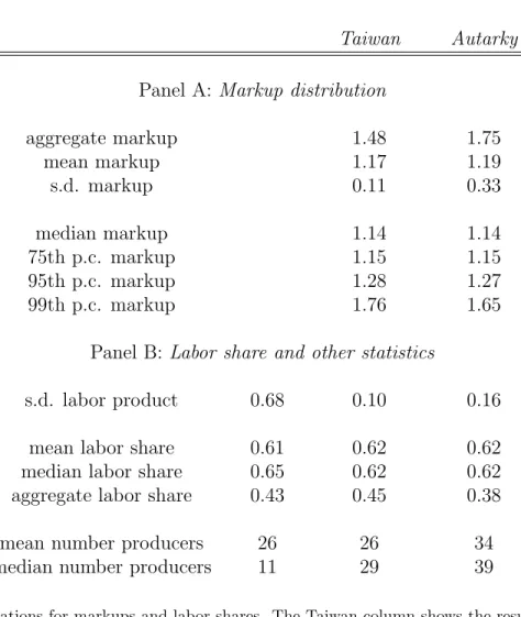
Strong concentration within sectors. Panel A of Table 1 shows that there is a high degree of concentration among domestic producers in individual 7-digit sectors. The average share of the largest seller in any given industry is equal to 0.45, only slightly greater than the median share of 0.39.

⁸

The mean (median) inverse Herfhindhals measures of concentration are equal to 7.3 (4.0), much lower than the average number of producers in any given sector.

Panel A of Table 1 also reports moments of the overall distribution of sectoral shares of domestic producers. These sectoral shares, unlike those discussed above, reflect sales by both domestic producers and imports. The average sectoral share of a domestic producer is 2.9%, whereas the median producer has a share of slightly below 0.4%. The distribution of shares is heavily fat-tailed : the 95th percentile of this distribution is equal to about 14% and the 99th percentile is equal to about 46%. The pattern that emerges is thus one of very strong concentration. Although many producers operate in any given 7-digit sector, most of these producers are small; a few large producers account for the bulk of any sector’s sales.

Strong unconditional concentration. Panel A of Table 1 also reports several statistics that capture the degree of concentration across all establishments. As documented in many other studies, employment and value added are strongly concentrated in the few large es- tablishments. The share of value added and wage bill accounted for by the largest 1% of producers is equal to 48% and 32%, respectively. Similarly, the largest 5% of all producers account for almost two-thirds of all value added and about one-half of all labor spending in Taiwanese manufacturing.

The labor share is negatively correlated with the sectoral share. We measure the labor share of producer

i

as

w_il_i/p_iy_i,

where

w_il_i

is the producer’s wage bill and

p_iy_i

their

8The sectoral statistics weigh each sector by its sales share.

value added: revenue net of intermediate inputs. To see the strong correlation between labor and sectoral shares, we find it useful to compare the aggregate labor share in Taiwan manufacturing (the sales-weighted average of individual producer labor shares) with the simple unweighted average.

The unweighted average labor share in the Taiwanese data is equal to 0.61. However, the aggregate labor share

W L

P Y

=

X

i

w_il_i p_iy_i

p_iy_i P

i⁰p_i⁰y_i⁰,

is much lower, equal to only 0.43.

⁹

This pronounced difference between the average and aggregate labor share emerges because, just as in the model, firms in the data that have high sectoral shares are also firms with low labor shares.

Another way to confirm this pattern is to regress producer labor shares on their sectoral shares. The point estimates imply that the labor share of a producer with a sectoral share of zero — essentially the median producer — is equal to 64%. By contrast, the labor share of a producer with a sectoral share of one-half is equal to 41%, i.e., 50% lower.

Is this correlation due to differences in capital intensities? One concern with our focus on labor shares is that differences in labor shares might really be due to firm-level differences in capital intensity rather than markups. To examine this, we suppose that firms have the technology

y_i

=

a_ik_i^αil^1−α_i ⁱ

and use data on plant capital stocks to calculate the sum of the labor and capital share. In the model, the sum of the labor and capital share is inversely related to markups but, unlike the labor share, is independent of the producer’s capital intensity,

α_i

:

w_il_i

+

rk_i p_iy_i

= 1

m_i.

To compute this object, we assume a user cost of capital,

r, equal to 0.15 which implies that

the median producer has a capital intensity,

α_i

, equal to 0.33.

¹⁰

Using the sum of the capital and labor shares we find, once again, that the implied aggregate markup is 40% larger than the average markup. Thus, differences in capital intensities alone do not account for the relationship between labor shares and sectoral shares.

9The manufacturing labor share is from the 2001 Taiwan National Statistics statistical tables, Table 23.

This measure, unlike our plant-level database, also includes benefits and proprietors’ income to compute labor compensation. See the Taiwan National Statistics data appendix, page 478, for further details.

10Our numbers are, however, very robust to reasonable perturbations ofr.

4 Quantifying the model

We now discuss how we use the Taiwanese data to pin down the key parameters of our model.

4.1 Overview

In the model, two key factors determine the size of the gains from trade: (i) the extent of initial misallocation, and (ii) the pattern of comparative advantage. These factors are governed by the amount of dispersion in productivity within and across countries, and by the elasticity parameters

γ

and

θ. We discipline our model along these dimensions as follows.

We choose a distribution of productivities that allows the model to reproduce the amount of concentration within individual sectors as well as the size distribution of establishments in Taiwan. We choose the elasticity parameters

γ

and

θ

so that the model reproduces standard estimates of the Armington elasticity used in the trade literature and the relationship between producers’ cost shares and sectoral shares in the data. Together, the productivity distribution and the elasticities

γ, θ

largely determine the amount of misallocation. Finally, the pattern of comparative advantage is largely determined by the cross-country correlation in producer- level productivity in individual sectors, which we pin down using data on the amount of intra-industry trade.

4.2 Productivity distribution

The distribution of producer-level productivities plays a key role in our analysis. Within a given country, the distribution of

a_ij

determines the pattern of concentration in individual sectors and the size distribution of producers. This, in turn, determines the degree of misal- location in the economy. Across countries, the correlation between

a_ij

and

a^∗_ij

determines the extent to which opening up to trade exposes highly productive domestic producers to com- petition from foreign producers. If Home and Foreign productivities are strongly correlated in any given sector, opening up to trade implies that even the largest domestic producers are exposed to strong foreign competition and are forced to reduce markups. In contrast, if Home and Foreign productivities are weakly correlated, trade does not much affect the amount of competition and thus has little effect on markups.

In standard trade models,

¹¹

productivity draws are assumed independent across coun- tries. Since the pattern of comparative advantage plays a key role in determining the pro-

11For example,Eaton and Kortum(2002) orBernard, Eaton, Jensen and Kortum(2003).

competitive gains from trade, we allow for dependence between Home and Foreign produc- tivities and study its effect on the gains from trade.

Joint distribution. Let

H(a, a^∗

) denote the joint distribution of productivities and let

F

(a) and

F

(a

^∗

) denote the (common) marginal distributions. We write the joint distribution:

H(a, a^∗

) =

C(F

(a), F (a

^∗

)), (21) where the copula

C

is the joint distribution of a pair of uniform random variables

u, u^∗

on [0, 1] and can be written:

C

(u, u

^∗

) =

H(F⁻¹

(u), F

⁻¹

(u

^∗

)). (22) In short, the copula governs the pattern of dependence between

a

and

a^∗

leaving the marginal distribution

F

(a) free to match within-country productivity statistics.

Marginal distribution. Given draws

u_ij

and

u^∗_ij

from

C

(u

_ij, u^∗_ij

), we set

a_ij

=

F⁻¹

(u

_ij

) and

a^∗_ij

=

F⁻¹

(u

^∗_ij

) and choose the (inverse) marginal distribution

F⁻¹

(u) to match the pattern of concentration in the Taiwanese data. In particular, we assume:

F⁻¹

(u) =

(

(1

−u)⁻

1

µL

if

u <

1

−p_H

(1

−u)⁻

1

µH

if

u≥

1

−pH

.

(23)

This distribution, which we refer to as the double Pareto, allows us to simultaneously match the fat-tailed size distribution of producers in the data and the amount of concentration in individual sectors. A small fraction

p_H

of producers draw their productivity from a fat-tailed Pareto with shape parameter

µ_H < µ_L

, while the rest of producers draw from a thin-tailed Pareto, thus allowing us to capture the size distribution at both the upper and lower tails.

¹²

The robustness section below studies an economy with a single Pareto marginal and illustrates the failure of that distribution to account for the data.

Copula. We use a Gumbel copula to control the cross-country dependence in productivity draws. This is a widely used copula that allows for dependence even in the right tails of the distribution:

C

(u, u

^∗

) = exp

−

[(− log

u)^ρ

+ (− log

u^∗

)

^ρ

]

^1ρ

, ρ≥

1. (24)

12We have also redone our analysis with a marginal distributionF(a) that is a binomial mixture of Paretos and obtained essentially identical results. We prefer the specification above since it can match the data with one fewer parameter than the binomial mixture and also because an inverse is available in closed form.

The parameter

ρ

controls the amount of dependence, which, as usual when working with fat-tailed distributions, we summarize using Kendall’s

τ

.

¹³

As with a conventional linear correlation coefficient, Kendall’s

τ

is scaled so that

τ

= 0 corresponds to independent random variables while

τ

= 1 corresponds to perfect dependence.

To highlight the role of dependence between Home and Foreign productivity draws, our analysis below starts by reporting the welfare gains from trade for two extreme parameter- izations:

τ

(ρ) = 1 and

τ

(ρ) = 0. It turns out that the choice of the other parameters of the model is not very sensitive to the value of

ρ. We therefore calibrate all the model’s

parameters assuming

τ

(ρ) = 1, and then keep those parameters fixed as we vary the amount of dependence in our experiments.

¹⁴

4.3 Calibration

Assigned parameters. We assume the utility function:

U

(C, L) = log

C

+

ψ

log (1

−L).

We choose a value for

ψ

to ensure

L

= 0.3 in the steady-state, implying a Frisch elasticity of labor supply equal to 2.33, in line with the findings of Rogerson and Wallenius (2009).

The period length is one year. We assume a time discount factor of

β

= 0.96 and a capital depreciation rate of

δ

= 0.10. The elasticity of output with respect to physical capital is

α

= 1/3.

¹⁵

We set the tariff rate

ξ

to 6.4%, which is the OECD estimate for Taiwanese manufacturing.

Productivity parameters and fixed costs. We choose the parameters

µL, µH, pH

of the double Pareto distribution, the fixed costs of selling in the domestic and foreign markets,

F_d

and

F_f

, and the number of technologies within a sector,

N

, to match key concentration

13Defined by:

τ≡4 Z 1

0

Z 1

0

C(u, u^∗)dC(u, u^∗),

which for the Gumbel distribution evaluates toτ = 1−1/ρ.

14Recalibrating all parameters as we varyτ(ρ) produces nearly identical results.

15As in Collard-Wexler, Asker and De Loecker (2011) and other studies of productivity dispersion, in our theoretical model we abstract from differences in capital and labor intensities, α, across sectors. Since markups affect the labor and capital wedges identically, and sinceαonly affects the relative weight on the two wedges, allowing for heterogeneity inαdoes not change the model’s implications for TFP and the aggregate level of markups in (16) and (17) above.

statistics in the Taiwanese data. Panel A of Table 1 reports the moments and the counterparts for our benchmark model. Panel B reports the parameter values that achieve this fit.

Our model successfully reproduces the amount of concentration in the data. The largest 7-digit producer accounts for an average 49% of that sector’s domestic sales (45% in the data).

The model also reproduces well the heavy concentration in the tails of the distribution of sectoral shares, with the 95th (99th) percentile share being equal to about 14% (46%) in both the data and the model. Finally, as in the data, the model produces a very fat-tailed size distribution of establishments: the top 1% and 5% of all producers in the data account for almost one-third and two-thirds of the total value added and wage bill, numbers close to those in Taiwanese manufacturing.

In the data, 25% of producers export. To match this fact, the model requires an export fixed cost

Ff

equal to 4.5% of steady-state labor. The fixed cost to operate domestically,

Fd,

is equal to 2.2% of steady-state labor. This level of the fixed cost is required for the model to reproduce the distribution of sectoral shares at the lower end of the spectrum. Absent this fixed cost, the model would predict a much smaller average sectoral share, since many very small producers would operate.

Finally, the distribution of productivity is highly fat-tailed. Although most producers draw from a Pareto with relatively thin tails,

µ_L

= 3.83, a few producers,

p_H

= 0.35%, draw from a very fat-tailed Pareto with

µ_H

= 1.5. Our Appendix shows that the model’s ability to fit the concentration in the data worsens significantly for greater values of

µ_H

.

Estimating

θ.

In the presence of fixed labor costs of production, the relationship between labor shares and sectoral shares predicted by the model, equation (13), generalizes to:

wl_i piyi

= (1

−α)

1

−

1

γ

−

(1

−α)

1

θ −

1

γ

ω_i

+

wF_d piyi

,

(25)

where

wl_i

is the wage bill for producer

i,p_iy_i

is its value added,

¹⁶ ω_i

is that producer’s share in its own sector, and

wF_d

is the fixed cost, assumed common to all producers. Now consider a regression of labor shares

wl_i/p_iy_i

on sectoral shares,

ω_i

, and inverse value added, 1/p

_iy_i

as in (25). For a given value of the within-sector elasticity

γ, the

ratio of the slope coefficient to the intercept uniquely determines

θ.

16Since we abstract from intermediate inputs in the model, we use data on value added (revenue net of intermediate inputs) as a proxy for sales. We calculate sectoral shares,ωi, using revenue data, however.