Breakdown of Anderson localization in the transport of Bose-Einstein condensates through one-dimensional disordered potentials

(1)

Breakdown of Anderson localization in the transport of Bose-Einstein condensates through one-dimensional disordered potentials

Julien Dujardin,¹Thomas Engl,²and Peter Schlagheck¹

1D´epartement de Physique, University of Liege, 4000 Li`ege, Belgium

2Institut f¨ur Theoretische Physik, Universit¨at Regensburg, D-93040 Regensburg, Germany (Received 23 October 2015; published 13 January 2016)

We study the transport of an interacting Bose–Einstein condensate through a 1D correlated disorder potential.

We use for this purpose the truncated Wigner method, which is, as we show, corresponding to the diagonal approximation of a semiclassical van Vleck–Gutzwiller representation of this many-body transport process.

We also argue that semiclassical corrections beyond this diagonal approximation are vanishing under disorder average, thus confirming the validity of the truncated Wigner method in this context. Numerical calculations show that, while for weak atom-atom interaction strengths Anderson localization is preserved with a slight modification of the localization length, for larger interaction strengths a crossover to a delocalized regime exists due to inelastic scattering. In this case, the transport is fully incoherent.

DOI:10.1103/PhysRevA.93.013612

I. INTRODUCTION

Localization phenomena in disordered systems highlight the fundamental role of interference of wave propagation [1].

A particular example of this is Anderson localization [2] (AL) describing the metal-insulator quantum phase transition in a 3D medium containing random impurities. The waves are coherently scattered over the impurities several times and yield to waves with an exponential profile resulting in a suppression of transport. Anderson localization has been experimentally observed with light in diffusive media [3] and in photonic crystals [4], with microwaves [5], and with sound waves [6].

The recent progress in the field of ultracold atoms has opened the possibility to experimentally study AL with a Bose-Einstein condensate (BEC), both in momentum space [7]

with aδ-kicked BEC [8] as well as in real space with the direct observation of exponential tails of the density profiles [9,10].

The use of a BEC to study AL is very appealing since it is possible to precisely tune the different properties of the BEC such as the two-body interaction strength between bosonic atoms via Feshbach resonances [11–13]. Research in the field of localization of bosonic atoms is motivated by the direct analogy with the electronic counterpart [14–17] and the perspective to realize bosonic atomtronic devices [18–21]

such as an atomic transistor. In this case the interplay between localization effects due to impurities and two-body interaction can play a major role in transport properties.

An accurate and numerically efficient theoretical description of transport process in such an open system faces the challenge of dealing with a many-body system with a potentially high number of atoms. The size of the associated Hilbert space renders techniques such as exact diagonalization or density matrix renormalization group (DMRG) methods inefficient or even practically impossible with the computational resources that are nowadays available. On the other hand, in the mean-field limit, corresponding to a high number of atoms and a weak two-body interaction, it is possible to describe the dynamics of the BEC in an approximate manner using the nonlinear Gross-Pitaevskii (GP) equation.

This limit has been extensively studied in the context of

bosonic transport and localization, both from the scattering perspective [22–30] as well as in the framework of wave packet expansion processes [31–35]. Furthermore, it has been shown that, even for weak interactions between atoms, inelastic scattering processes are not negligible [36,37] thus potentially invalidating results obtained by the GP mean-field description. Several methods exists to take into account effects beyond the mean-field description. In particular a Bogoliubov description [38–47] seems very promising and offers the advantage of allowing for analytical solutions.

As was done in Refs. [24,30] we study, in this paper, the effect of atom-atom interactions on AL in the context of an atom laser [48–51] which consists of a reservoir of atoms that are outcoupled into a waveguide. The atoms eventually encounter the disordered region within this waveguide. We describe the system with the truncated Wigner (tW) method [52–58] that essentially consists of representing the many-body bosonic quantum fields in terms of classical fields. This method has been successfully used to study several dynamical processes in closed systems; see, e.g., Refs. [59,60]. The steps towards a numerically efficient formulation of the truncated Wigner method for a one-dimensional open system have been achieved in Refs. [61,62]. Moreover, the tW method has been shown to correctly model inelastic scattering [62] and to yield consistent results in the continuous limit [63].

The main object of our study is the breakdown of AL in correlated disorder potentials due to the presence of atom-atom interaction, which is to be investigated with the truncated Wigner method. To this end, we first describe, in Sec.II, the one-dimensional transport scenario we are interested in and then, in Sec. III, how the truncated Wigner method can be implemented. In Sec.IV, using a semiclassical approach [64], we calculate the leading corrections to the so-called diagonal approximation, the latter being equivalent to the truncated Wigner method [63]. These leading corrections are shown to be negligibly small when performing a disorder average.

We finally compare numerically, in Sec.V, the transmission and the density profiles across Gaussian-correlated disorder potentials provided by the mean-field GP description and the truncated Wigner method.

(2)

x E

BEC

L

|1,−1

|1,0

¯hωrf

μ (a) BEC

(b)

(c)

S

Scattering region

Left lead Right lead

FIG. 1. (a) Typical atom laser configuration inspired from Ref. [48], consisting of a BEC within a magnetic trap of atoms and an optical waveguide generated by a spatially focused light field. (b) The atoms in the reservoir are outcoupled from the trapped state|F,mF = |1,−1to the untrapped state|1,0thanks to a radio-frequency field of energy ωrf. In the untrapped state, atoms are confined in the waveguide rendering the propagation quasi-one-dimensional in the longitudinal x direction. A disorder potential can then be engineered to study transport properties across it. (c) The corresponding theoretical description involves a spatial grid that is described in Sec.II B. We suppose, in addition, that the potential has a finite support of lengthLand that atoms are interacting only within this support.

II. GUIDED ATOM LASERS A. Theoretical description

Let us consider a typical atom laser experiment such as the one reported in Ref. [48], the working principle of which is depicted in Fig.1. The condensed ⁸⁷Rb atoms are trapped in a magnetic trap and constitute thereservoircontaining a high numberN of atoms that are ideally in a perfect condensate maintained at zero temperature. Theses atoms are spin polar- ized in the trapped state |F,mF = |1,−1 with energy E₁. To release the atoms, i.e., transfer them to an untrapped state

|1,0with energyE₀, a radio-frequency field consisting of a nearly resonant electromagnetic wave at energyω_rf(∼2π· GHz) is used to couple the state |1,−1 to the state |1,0.

These atoms are insensitive to the external magnetic field and propagate in the waveguide. The chemical potential is given byμ=E₁−E₀−ω_rfand corresponds to the kinetic energy per atom. The propagation of atoms can thus be considered as a free quasi-one-dimensional motion. It is then possible to engineer a correlated disorder potential (see, e.g., Ref. [65]) with a finite extentLand study the suppression of transport.

In order to represent the atoms in the atom laser system, we define, within second quantization, the field operator of the

atoms in the trap ˆφm_F=−1(r,t) corresponding to the atoms in the hyperfine state|1,−1and the field operator of the atoms in the waveguide ˆψ_m_F=0(r,t) corresponding to the atoms in the hyperfine state|1,0as

ψˆ_m_F=0(r,t)=ψ(r,tˆ )e⁻^iμt/, (1a) φˆm_F=−1(r,t)=φ(r,t)eˆ ⁻^i(μ⁺^ω^rf^)t/. (1b) The corresponding evolution equation for the field operators in the Heisenberg representation can be written as

i∂

∂tψ(r,tˆ )=

−² 2m

∂²

∂r² −μ+V_opt(r)

ψ(r,tˆ )

+Uψˆ^†(r,t) ˆψ(r,t) ˆψ(r,t)+D(t) ˆφ(r,t), (2a) i∂

∂tφ(r,tˆ )=

−² 2m

∂²

∂r² +V_trap(r)

φ(r,tˆ )

+D^∗(t) ˆψ(r,t), (2b) where V_opt is the optical potential including the waveguide and V_trap is the magnetic trapping potential. We consider a slowly varying transverse confinement frequency ω_⊥(x) of the waveguide in such a way that the spatial variations of this potential cannot induce excitation of transverse modes.

We take into account the interactions between the atoms by the mean of a low-energy contact pseudopotential [66].

The interaction strength between the atoms in state|1,0 is U =4π²aS/m, where aS is the s-wave scattering length.

The coupling strength between the reservoir and the guide is defined as D(t) and is adiabatically ramped from zero to a constant valueD.

Assuming that the atoms in the reservoir are all in the ground state, we can decompose the associated field operator as φ(r,t)ˆ =φ₀(r) ˆψ_S(t). During the coupling process, we suppose that only the transverse ground modeχ₀(y,z) is populated. We can therefore decompose the field operator associated with the waveguide as ˆψ(r,t)=χ₀(y,z) ˆψ(x,t). Finally we neglect both the (intraspecies) interaction between (mF = −1) atoms in the reservoir and the (interspecies) interaction between (mF = −1) atoms in the reservoir and (mF =0) atoms in the waveguide, assuming that the latter do not play any role in the vicinity of the disordered system. These assumptions allow us to simplify Eqs. (2) yielding

i∂

∂tψ(x,t)ˆ =H0ψ(x,tˆ )+g(x) ˆψ^†(x,t) ˆψ(x,t) ˆψ(x,t) +K(x,t) ˆψ_S(t), (3a) i∂

∂tψˆS(t)=

dx K^∗(x,t) ˆψ(x,t), (3b) where we define

H0 =Hk−μ+V(x), (4a) Hk = −²

2m

∂²

∂x², (4b)

g(x)=2ω_⊥(x)aS, (4c) K(x,t)=D(t)

dy dz χ₀^∗(y,z)φ₀(r). (4d)

(3)

B. Discretization of space

Following the procedure described in Ref. [63], we dis- cretize space by constructing a grid along the one-dimensional guide by introducing an energy cutoff in momentum space at p= ±π/δ. We modifyHkaccordingly by

H^δk=Eδ[1−cos(δp/ˆ )], (5) with ˆp= −i∂_x and E_δ =²/mδ². The eigenstates of the modified Hamiltonian ˜φ_k(x)=exp(ikx)/√

2πare identical to the ones ofHkand the associated eigenvalues now read

Ek=Eδ[1−cos(kδ)], (6) where k∈[−π/δ,π/δ]. In the continuous limit, i.e., for kδ→0, we haveH^δ₀→H0 and the eigenvalues tend to the continuous ones:Ek=²k²/2m.

Defining an effective Wannier basis composed of spatially localized functions

φ_l(x)= δ

2π π/δ

−π/δ

φ˜_k(x)e^ilkδdk (7) forl∈Z, and the corresponding bosonic annihilation ˆψl and creation ˆψ_l^†operators, we have

ψ(x)ˆ = ^∞

l=−∞

φ_l(x) ˆψ_l. (8) In addition, we suppose that the source is located at positionxS

corresponding to the sitelS. As a consequence, we can define a coupling strengthκ(t) on sitelSas

K(x,t)=κ(t)φl_S(x). (9) Inserting Eqs. (8) and (9) in the evolution equations (3), we obtain, in the limitδ→0,

i∂ψˆl(t)

∂t =(Eδ+Vl−μ) ˆψl(t)−Eδ

2 [ ˆψl−1(t)+ψˆl+1(t)]

+glψˆ_l^†(t) ˆψl(t) ˆψl(t)+κ(t)δl,l_SψˆS(t), (10a) i∂ψˆ_S(t)

∂t =κ^∗(t) ˆψl_S(t), (10b)

with Vl=V(lδ), gl=g(lδ)/δ, Eδ =²/(mδ²), where the coupling strength is well approximated by κ(t) K(xS,t)/√

δ. A visual representation of this discretization scheme is provided in Fig.1(c).

III. TRUNCATED WIGNER METHOD

The truncated Wigner method [52–58] has been recently adapted to deal with many-body bosonic scattering processes in the context of a guided atom laser [62,63]. Describing the latter with the evolution equations defined by Eqs. (10), applying the tW method effectively amounts to solving the equations [62]

i∂ψl

∂t =(Eδ+Vl−μ)ψl−Eδ

2 (ψl+1+ψl−1) +gl(|ψl|²−1)ψl+κ(t)ψSδl,l_S, (11a) i∂ψS

∂t =κ^∗(t)ψlS, (11b)

where ψ_l andψ_S are the classical fields associated with site land the source, respectively. Denoting byA= {S,0,±1,± 2, . . .}the ensemble of sites of the system, we can express the corresponding classical Hamiltonian H_cl(ψ,ψ^∗), where ψ =(ψα)α∈A, as

H_cl(ψ,ψ^∗)=

l∈Z

(Eδ+Vl−μ)|ψl|²+g_l

2|ψl|²(|ψl|²−2)

−Eδ

2 (ψ_l^∗₊₁ψl+ψ_l^∗ψl+1)

+κ^∗(t)ψ_S^∗ψ_l_S+κ(t)ψ_l^∗_Sψ_S. (12) The classical fields ψl and ψS correctly sample, in the framework of the tW method, the initial quantum state.

More specifically, for the empty waveguide, the initial field amplitudes att =t₀read

ψ_l(t₀)=(Al+iB_l)/2, (13) withA_l andB_lreal, independent Gaussian random variables with unit variance and zero mean; i.e., for eachl,l∈Z we have

Al=Bl =0, (14a)

A_lA_l=B_lB_l =δ_l,l, (14b)

AlBl =0, (14c)

where the overline denotes the average over the random variables. Since|ψ_l|²=1/2, this sampling effectively amounts to having half a (pseudo)particle on each site of the numerical grid from the classical point of view. The source of atoms is a BEC with a high numberN of atoms and can therefore be represented as a coherent state|ψ_S⁰. AsN is very large, the relative uncertainty of both the amplitude|ψ_S⁰| =√

Nand the associated phase of the source are negligibly small. We therefore treat the source term completely classically and set ψ_S⁰=√

N without loss of generality. Supposing, in addition, that the couplingκ(t) tends to zero such thatN|κ(t)|²remains finite, we can safely neglect the depletion of the source or any back-action of the waveguide to the source. In this context, the evolution of the source can be neglected and we can focus on the evolution of the field in the waveguide only. The equation of evolution finally reads

i∂ψl

∂t =(Eδ+V_l−μ)ψl−Eδ

2 (ψl+1+ψ_l₋₁) +gl(|ψl|²−1)ψl+κ(t)√

N δl,l_S. (15) The observables such as the density and the current are then computed through the statistical average over all classical initial states. This average will be denoted by an overline as in Eqs. (14). For instance, the total densityρ(x =lδ,t) and

(4)

currentj(x=lδ,t) at positionx =lδare computed through ρ(lδ,t)= 1

δ

|ψ_l(t)|²−1/2

, (16)

j(lδ,t)= i

2mδ²(ψ_l^∗₊₁(t)ψl(t)−ψ_l^∗(t)ψl+1(t)). (17) The half particle that is added through the sampling of the initial state is subtracted after the time propagation. In the tW framework, it is possible to decompose the total current and the total density into coherent and incoherent contributions. The first contribution comes from the coherent parts of the density ρ^coh(x =lδ,t) and the currentj^coh(x =lδ,t) at positionx= lδ, which represent the condensed atoms. They can be written as

ρ^coh(lδ,t)= ψl(t) ²/δ, (18) j^coh(lδ,t)= i

2mδ²(ψ_l^∗₊₁(t)ψl(t)−ψ_l^∗(t)ψl+1(t)). (19) The incoherent parts of the densityρ^incoh(x =lδ,t) and current j^incoh(x =lδ,t) at positionx=lδare defined as the difference between the total part and the coherent part. They read

ρ^incoh(lδ,t)=n(lδ,t)−n^coh(lδ,t), (20) j^incoh(lδ,t)=j(lδ,t)−j^coh(lδ,t). (21) The total transmission is then naturally defined as the ratio of the total current in the downstream region and the stationary current j^∅ for a homogeneous waveguide with a vanishing atom-atom interaction. It reads

T = lim

t→∞j(t)/j^∅, (22)

where we dropped the spatial dependence of the current. The stationary currentj^∅is given by

j^∅= δ

N|κ|²

√μ(2Eδ−μ). (23) In the same way, one can define the coherent part of the transmission and the incoherent part of the transmission as

T^coh= lim

t→∞j^coh(t)/j^∅, (24a) T^incoh= lim

t→∞j^incoh(t)/j^∅. (24b)

Finally, we can also evaluate the stationary densityρ^∅in the case of a homogeneous waveguide with vanishing atom-atom interactions as

ρ^∅= 1 δ

N|κ|²

μ(2Eδ−μ). (25) For the rest of the paper, we will consider that the on- site potential V_l and the contact interaction strength g_l are nonvanishing only in a finite region of space. The latter region will be called the scattering region and the regions on the left- and right-hand sides of it will be named left andright leadsin close analogy with electronic mesoscopic physics [see Fig.1(c)]. An efficient way to numerically model the decay of atoms to the leads is provided by the method of smooth

exterior complex scaling [61]. This method transforms the infinite scattering system into a finite open system. The initial quantum fluctuations of the leads take the form of a time- dependent quantum noise that enters into the scattering region by the first and the last site [62]. This allows one to efficiently simulate scattering processes of guided matter waves using the tW method [62].

IV. VALIDITY OF THE TRUNCATED WIGNER METHOD As was shown in Ref. [63], the tW method corresponds to the diagonal approximation [67] in the framework of the semiclassical van Vleck–Gutzwiller description [68] of the bosonic many-body system. This insight offers a scheme for assessing the validity of the tW approach. We have to require, on the one hand, that the actions of the trajectories involved in the van Vleck–Gutzwiller approach be large compared to the size of Planck’s constant, in which case the stationary phase approximation of the Feynman propagator can be justified. The validity of the diagonal approximation, on the other hand, can be granted if the classical dynamics is fully chaotic and if some sort of (energetic or disorder) averaging of the observables of interest is performed.

It is known, however, that there exist systematic and robust corrections beyond the diagonal approximation which may significantly affect quantum transport processes. These are, on the one hand, induced by coherent backscattering effects, the relevance of which for closed bosonic many-body systems has been studied in detail in Ref. [64]. On the other hand, the apparent violation of norm conservation due to coherent backscatttering is compensated by loop contributions arising from Sieber-Richter trajectory pairs [69–78]. The purpose of this section is to investigate these corrections in more detail for the bosonic many-body transport problem under consideration.

We shall show in the end that they do not matter in the context of open atom-laser-like scattering systems.

A. Semiclassical van Vleck–Gutzwiller theory for Bose-Hubbard systems

Generally, the semiclassical approach can be understood as an expansion in a small parameter, namely the effective Planck constanteff which vanishes in the classical limit. In a second quantized many-body theory, the role of this effective Planck constant is played by the inverse of the total number of particles N; i.e., we identifyeff =1/N. Applying the semiclassical theory to calculate the expectation value of some observable Oˆ then yields results of the form [73,79]

Oˆ(t)=O_cl(t)+^∞

k=1

^k_effO_corr^(k)(t), (26) whereO_clis the result of the corresponding classical theory and O_corr^(k) is thekth-order quantum correction due to interference between certain classical paths, which can typically expressed in terms ofO_cl. In the case considered here, it will turn out that O_clis given by the truncated Wigner result and all quantum corrections vanish.

The starting point of the semiclassical approach is the path integral representation of the propagator ˆK(t)=exp(−iH t /ˆ ) in a certain basis. For many-body systems, the most natural

(5)

basis is constituted by the Fock states

|n ≡ |nS ⊗ |. . . ,n₋₁,n₀,n₁, . . .

=

α

√1 nα!

ψˆ_α^†n_α

|0, (27) which are determined by the occupation numbers (i.e., the numbers of atoms)nαon the individual sitesα(including the source) and which are generated by applying the associated creation operators to the so-called vacuum state|0. However, it turns out that the semiclassical approximation for the propagator in Fock states also requires large occupations of each individual site [64,80] (typicallyn_α2 [81]) which is not granted in the scattering scenario considered here.

A possibility to circumvent this problem is to use the quadraturerepresentation,

K(A^f,Aⁱ;t)= A^f|e⁻ⁱ^{H t/}^ˆ |Aⁱ, (28) where the quadrature states|Aare defined by the eigenvalue equation [82]

1

2( ˆψ_α+ψˆ_α^†)|A =Aα|A (29) and can be expanded in Fock states according to

|A =

n

α

exp

−A²_α 2ⁿ^αn_α!√

π/2Hn_α(√ 2An_α)

|n. (30) The analogy between these quadrature states and the position states of the harmonic oscillator is completed by the closure relation

ˆ1=

α

dA_α|AA| (31) and their overlap

A|A =

α

δ(Aα−A_α). (32) Finally, the action of an annihilation or creation operator on a quadrature state is given by

ψˆα|A =

Aα+1 2

∂

∂A_α

|A, (33a)

ψˆ_α^†|A =

A_α−1 2

∂

∂Aα

|A. (33b)

If the total number of particles in the scattering region is large enough [83], the path integral for the propagator in quadrature representation, given by Eq. (28), can be evaluated in a stationary phase approximation yielding the semiclassical propagator [64,68,84]

K

A^f,Aⁱ;t

γ

Dγ(A^f,Aⁱ;t)e^iR^γ(^A^f^,Aⁱ^;t)^/, (34) where the sum runs over all trajectoriesγ between|A and

|Athat satisfy the classical equations of motion i∂ψα

∂t (t)= ∂H_cl(ψ^∗,ψ)

∂ψ_α^∗ , (35)

(a) (b)

(c) (d)

FIG. 2. While for an individual system one would have to take into account all trajectories in the sum over partner orbits [(a)], under disorder average only certain partner trajectories are selected [(b)–(d)]. These pairs are, ordered from largest to smallest contributions, the diagonal approximation [(b)], coherent backscattering contributions [(c)], and loop contributions [(d)].

which are the same as in Eq. (11) with the classical Hamilto- nianH_clfrom Eq. (12), and under the boundary conditions on the real parts ofψ,

Reψα(0)=Aⁱ_α, (36a) Reψα(t)=A^f_α. (36b) It is this sum together with the phase factor given by the action of the trajectoryγ,

Rγ(A^f,Aⁱ;t)= t

0

ds

2B· d

dsA−H_cl(ψ^∗(s),ψ(s))

, (37) that accounts for the interference effects lying beyond the truncated Wigner approach, the latter being, in the sense of N→ ∞, the classical limit of the quantum theory [63].

HereA(s) andB(s) are the real and imaginary part ofψ(s), respectively. Finally, the semiclassical amplitude is given by

Dγ(A^f,Aⁱ;t)=

det 1

−2π i

∂²Rγ(A^f,Aⁱ;t)

∂A^f∂Aⁱ

=

det 1

π i

∂B(0)

∂A^f

, (38)

where the derivatives of the action with respect to the initial and final quadratures

∂Rγ

∂Aⁱ = −2B(0), (39a)

∂Rγ

∂A^f =2B(t) (39b)

have been used.

(6)

In order to proceed further, it is important to know the initial state |ψ⁰ of the system. According to the considerations in Sec.III, it will be assumed that the initial state is given by the vacuum in the waveguide and a coherent state in the source,

|ψ⁰ = ψ_S⁰

⊗ |0, (40) where due to the gauge freedomψ_S⁰=√

N can be chosen to be real.

Inserting the resolution of unity (31), using the action of annihilation and creation operators on quadrature states (33), as well as inserting the semiclassical approximation for the propagator (34) while letting the derivatives of the propagator act on the exponential only [85] then yields

ψˆ_l^†(t) ˆψ_l(t) =

α

2 π

dAⁱ_α

dA^f_α

×exp

−

l∈Z

Aⁱ_l

₂ +

Aⁱ_l

₂

− Aⁱ_S−√

N₂

− Aⁱ_S−√

N₂

×

γ₁:Aⁱ→A^f γ₂:Aⁱ→A^f

Dγ1D^∗γ₂exp i

R_γ₁−R_γ₂

×

ψ_l^(γ²⁾^∗(t)ψ_l^(γ¹⁾(t)−1 2δll

, (41)

where Eq. (39b) has been used and the superscript (γ1/2) indicates that the quantity is computed along the trajectory γ_1/2. The first exponential in Eq. (41) results from the overlap of quadrature states with the initial state and effectively reduces the integrations to a very small region, such that the initial quadratures Aⁱ,Aⁱ lie very close to each other. Following standard semiclassical perturbation theory [86], we therefore replaceAⁱwithAⁱin the definition of the trajectoriesγ₂and account for the induced error by expanding the action in the exponential up to linear order in the differenceAⁱ−Aⁱ. The integration overAⁱis then simply a Gaussian integral, which can be performed exactly yielding

ψˆ_l^†(t) ˆψ_l(t)

α

2

dAⁱ_α

dA^f_α

γ1,γ2:A→A^f

Dγ1Dγ^∗2

×exp

−2

α∈Z

Aⁱ_α2

+1 4

B_α^(γ¹⁾(0)+B_α^(γ²⁾(0)2

×exp

−2 Aⁱ_S+ i

2

B_S^(γ¹⁾(0)+B_S^(γ²⁾(0) −√

N ²

×exp i

R_γ₁−R_γ₂

ψ_l^(γ²⁾^∗(t)ψ_l^(γ¹⁾(t)−1 2δ_{l l}

. (42) This equation represents the starting point for the discussion of the diagonal approximation and the corresponding corrections provided by coherent backscattering and loop contributions.

B. Closed systems

Let us first consider the case of a closed disordered system with a finite number of sites, which could, e.g., describe an ultracold Bose gas that is contained within a finite optical lattice [64]. When performing a disorder average, the action differenceR_γ₁−R_γ₂arising in Eq. (42) varies strongly from one disorder realization to the next one, as long as the trajectoriesγ₁andγ₂are not correlated. Therefore, on average, most of the contributions to the double sum will cancel out and only pairs of trajectories that are close to each other during the whole evolution time will contribute. A short pictorial summary of the possible pairings is shown in Fig.2.

For such pairs of trajectories, one can safely neglect the tiny differences in the prefactorsDγ_j and amplitudesBα^(γ^j⁾(0) (j =1,2) between the two trajectories, such that only their action differenceR_γ₁_,γ₂ =R_γ₁−R_γ₂ is taken into account.

Equation (42) then becomes ψˆ_l^†(t) ˆψ_l(t)

α

2

dAⁱ_α

dA^f_α

γ:Aⁱ→A^f

|Dγ|²

×exp

−2

l∈Z

Aⁱ_l2

+

B_l^(γ⁾(0)2

×exp

−2 Aⁱ_S−√

N₂

−2

B_S^(γ⁾(0)₂

×

ψ_l^(γ)^∗(t)ψ_l^(γ ⁾(t)−1 2δl l

×

γ_p

exp i

Rγ ,γ_p

. (43)

Here the sum overγ runs over all possible trajectories while the second sum overγ_pincludes all partner trajectories whose actionsRγ_pare systematically correlated with the actionRγ of the trajectoryγ and whose contributions thereby survive the disorder average.

1. Diagonal approximation

The easiest possibility for the partner trajectoryγpto yield a nonvanishing contribution on average is to choose it to be the same as γ: γp =γ. This is known as the diagonal approximation [67] and has obviously a vanishing action difference. Then, by using the sum rule

α

dA^f_α

γ:A→A^f

|Dγ|². . .=

α

1 π

dBα

. . . ,

(44) which is a direct consequence of |Dγ|²=

|det[∂B^(γ⁾(0)/∂A^f]/π|, the integration over A^f can be transformed into an integration over B. This yields together with the integration overAⁱa Gaussian sampling over initial conditions, which are then evolved according to the equations of motion (11). The observable is then calculated from the thereby evolved state only. Thus with Eq. (44) the shooting problem, where the real parts of ψ at initial and final time are fixed, is transformed into an initial value problem, which

(7)

exactly yields the truncated Wigner method described in Sec.III[63].

2. Coherent backscattering

The second possibility for the partner trajectory γ_p is to choose it to be the time reverse of γ, provided the latter is not identical toγ (in which case the trajectory retraces itself in configuration space). Then obviously the action difference again vanishes. This kind of pairing requires that A^fAⁱ, i.e., that the trajectory comes back to its initial point. As such trajectories can thus be paired with themselves and with their time-reversed counterparts, their contributions to Eq. (43) are therefore enhanced by a factor 2 as compared to other trajectories. This yields a coherent enhancement of backreflection [64].

However, when considering single-particle observables such as the ones that we are focusing on here, the final quadra- tureA^fis integrated over, which leads to a suppression of the coherent backscattering enhancement (or, more precisely, to a reduction of this enhancement by a factor that is of the order of the number of accessible many-body states with the same number of particles and about the same energy as the initial state [64]). This need not be the case for more sophisticated observables: the inverse participation ratio in the quantum many-body space, for instance, is enhanced by a factor 2 as compared to its classical value [64]. Mean on-site densities and intersite currents, however, are not expected to be appreciably affected by coherent backscattering.

3. Loop corrections

Further possibilities for the partner trajectories have been found to be obtained by what is now known as loop contributions resulting from Sieber-Richter trajectory pairs [69–78], such as the one shown in Fig.2(d). These Sieber-Richter pairs consist of trajectories which in a certain very small region in phase space, the so-called encounter region, come close to their own time reverse. The partner trajectory closely follows thenγor its time reverse all along the trajectory, except within the encounter region where it switches from following γ to following its time reverse or vice versa.

Such loop contributions are generally arising in quantum systems with a chaotic classical dynamics where the existence of partner trajectories with the above properties is granted by the shadowing theorem. While they turn out to significantly affect, e.g., transport properties within mesoscopic systems [70,74–76,87] and the Loschmidt echo [88,89], they can be shown to vanish for the evaluation of single-particle observables in ordinary time-evolution processes taking place within closed generic systems [77,78,90], in close analogy with the absence of coherent backscattering contributions. This also holds for the Bose-Hubbard systems that are considered here, which exhibit a second constant of motion in addition to the total energy, namely the total number of particlesN. In AppendixA we show how to incorporate this additional conserved quantity.

C. Open systems

Open quantum many-body systems feature the complica- tion that their number of classical degrees of freedom (i.e., the

total number of Bose-Hubbard sites in our case) is infinitely large from a formal point of view, even if a discretization of the configuration space is employed. While the diagonal approximation can still be applied in this context without any further considerations [63], one has to be more careful with coherent backscattering and loop contributions.

On one hand, coherent backscattering contributions require the existence of trajectories that come back to their initial point, which is a very unlikely event to happen within an infinite system. Indeed, in our context of a guided atom laser, this would imply thatall atomsof the condensate come back to the reservoir after having explored the disordered region within the waveguide. Already from this point of view, one would expect that effects due to coherent backscattering in the many-body space are completely suppressed in open systems.

On a more rigorous level, it can be shown (see AppendixB) that in open systems the possibility of pairing a trajectory with its time-reversed counterpart requires self-retracing of the trajectory. This, however, implies that the trajectory would be identical with its time-reversed counterpart, which means that it does not contribute to coherent backscattering. Hence, coherent backscattering contributions do indeed vanish in the case of open systems.

A similar conclusion is obtained for the contributions of possible loop corrections within open systems. To investigate their relevance, it is convenient to employ a scattering approach in which the two semi-infinite left and right leads are formally separated from the finite scattering region which contains, as is illustrated in Fig. 1(b), the disorder potential as well as the coupling to the source. As the interaction strength is vanishing outside the scattering region, the dynamics in the leads can be exactly integrated yielding integro-differential (i.e., temporally delayed) decay terms as well as quantum noise terms in the effective tW description of the scattering region [61,62]. We show in AppendixB how to derive the corresponding semiclassical propagator describing the time evolution within the finite scattering system.

As the dynamics outside the scattering region is noninter- acting, the semiclassical approximation for the propagation in the leads is exact and can thus be represented by a single classical trajectory. Encounter regions where a trajectory comes close to its time-reversed counterpart in phase space may therefore arise only in the scattering region in which the presence of interactions can give rise to classical chaos [91,92].

The resulting exponential sensitivity of the classical time evolution with respect to variations of the initial conditions is already sufficient for the existence of Sieber-Richter pairs [69].

Their contributions to the time-dependent expectation values of single-particle observables can then again be evaluated following the standard theory of loops [71,72,74–78,90,93].

By virtue of the same arguments that are put forward in closed systems [77,78,90], we can again show that loop contributions vanish in the context of many-body scattering.

V. NUMERICAL RESULTS

A. Anderson localization of weakly interacting atoms We now apply the truncated Wigner method to investigate the transmission of the BEC across a disordered region of

(8)

0 100 200 kL

10^-5 10^-4 10^-3 10^-2 10^-1 10⁰

<T>

GPcoherent incoherent total

0 100 200

kL

50 100 200 0.05

0.1

(a) (b)

FIG. 3. Transmission versus the length L of the Gaussian- correlated disorder potential (45) with the parametersA=0.265k^3/2 and kσ=√

2 for the atom-atom interaction strengths (a) g= 0.00095μ/k and (b)g=0.048μ/k. The coherent, incoherent, and total transmissions obtained by the tW method are represented by (red) squares, (green) diamonds, and (blue) triangles, respectively, and the mean-field GP predictions for the transmission is shown by (black) circles. While for very weak interactions (a) the transmitted beam is fully coherent and subject to AL, a breakdown of AL is encountered at stronger interactions beyond a certain disorder length (b) yielding a fully incoherent beam in the transmitted region.

The maroon solid lines show fits of Eq. (46) to the decay of the transmission within the coherent regime, yielding the localization lengths kLloc28 in panel (a) and kLloc27 in panel (b). The orange line in the latter panel shows a fit of a 1/(1+L/L0) scaling of the transmission in the incoherent regime withkL010.8, which reproduces well the numerical data (as seen in the log-log plot in the inset).

finite lengthL. We specifically consider a Gaussian-correlated disorder potential that is generated in the same way as in Ref. [94], i.e.,

V(x)=²A m

L 0

√1

2π σ e⁻^(x−y)2^2σ² η(y)dy. (45)

Here, the parameter A controls the height of the disorder potential, σ is the correlation length, and η(y) is a Gaussian white noise with zero mean and unit variance, i.e., η(x)η(y) =δ(x−y), where · denotes the average over different realizations of the disorder. The potential is constructed such that it vanishes on average, i.e.,V(x) =0.

We shall choose the parametersA=0.265k^3/2andkσ=√ 2 in the following where we haveμ=²k²/(2m). The coupling to the source is tuned such that a steady-state density of ρ^∅ =√

2kwould be obtained within the waveguide if there were no disorder or interaction between the atoms.

Figure3(a)shows the coherent, incoherent, and total transmission of the condensate across the disorder potential (45) as a function of its lengthLin the presence of an artificially weak interaction strengthg=0.00095μ/k. We can directly notice that the coherent and total transmissions are nearly identical and agree very well with the transmission obtained from a mean-field GP calculation. The incoherent part of the transmission is suppressed by several orders of magnitude, but steadily increases withL, and we cannot exclude that it may eventually dominate the transport process for sufficiently long disorder regions.

A smoking gun of AL in disorder potentials is the dependence of the average transmission versus the lengthLof

the potential. More precisely, definingξ =L/L_loc, we have T(ξ) = e⁻^{ξ /4}

2 π ξ³

_∞

0

du u² cosh_u

2

exp −u²

4ξ

, (46) for the transmission of single particles across one-dimensional disordered regions [95], whereL_locis defined as thelocaliza- tion lengthwhich is proportional to the transport mean-free path [96]. This formula was shown to be valid also in the mean-field limit described by the GP equation [94], but does not take into account the possibility of depletion of the condensate beyond the mean-field approximation.

The maroon solid line in Fig. 3(a) shows a least-mean- square fit of Eq. (46) to the total transmission, yielding very good agreement with the numerical data. The coherent flux of atoms therefore exhibits AL when passing through the Gaussian-correlated disorder potential. Note that the numerically extracted value kL_loc28 of the localization length lies significantly below the theoretical value that would be predicted by the Born approximation [94,97]. This is not surprising since the latter requires²A/(mμk^3/2)1 to be valid, which is not satisfied in our case.

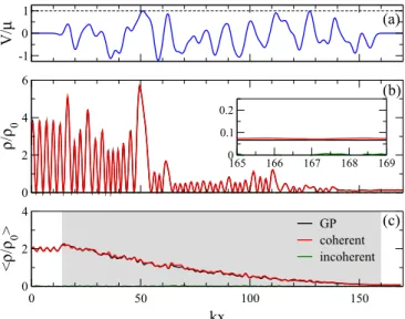
Figure 4 shows the corresponding density profile of the atom laser beam for a fixed length of the disorder potential, namelykL=141.42, still in the case of very weak interaction.

We can see that the GP and tW calculations yield nearly identical densities in the waveguide, both for individual disorder realizations [panel (b); the inset confirms that a stationary state has been reached] and on average [panel

-1 0 1

V/μ

0 2 4 6

ρ/ρ 0

0 50 100 150

kx

0 2 4

<ρ/ρ 0> ^GP_coherent

incoherent 165 166 167 168 169 0

0.1 0.2

(a)

(b)

(c)

FIG. 4. Density profiles for weak interaction g=0.00095μ/k and a final propagation time ofμT /=1000. Panel (a) shows one realization of the disorder potential generated according to Eq. (45) and (b) represents the stationary density of an incoming beam of atoms going through the disorder potential represented in (a) with an inset magnifying the transmitted beam. Panel (c) shows the disorder average of the density profile taking into account 1000 realizations of the disorder. The gray background helps the reader to locate the disorder region. We can clearly see that the transport process is fully coherent and that the mean-field GP description (black line) agrees well with the truncated Wigner method (red line for the coherent and green line for the incoherent part).

(9)

(c)]. One should point out that some fluctuations remain in the tW calculation, inherent to the stochastic nature of the technique.

B. Breakdown of Anderson localization

We now focus our attention on the transition to incoherent transport. In Fig. 3(b) we use the same parameter set as in Fig. 3(a) except for the interaction strength which is increased tog=0.048μ/k=0.034²/(mσ). This latter value would correspond to the case of ⁸⁷Rb atoms with the s- wave scattering lengtha_s 5.3 nm being confined in a harmonic waveguide with the transverse confinement frequency ω_⊥/(2π)=1.2 kHz, where we choose the correlation length of the disorder potential to be equal to the transverse oscillator length:σ =√

/(mω_⊥)0.31μm. One can directly see that for smallkLwe are still in the mean-field regime since the incoherent transmission is still several orders of magnitude below the coherent part. However, we now observe a rapid increase of the incoherent part of the transmission withkL. It becomes nonnegligible at aboutkL100, and forkL >100 the transport is fully incoherent.

The dark (maroon) solid line in Fig. 3(b)shows a fit of Eq. (46) to the numerically computed transmission data for kL <50 and the dark (maroon) dashed line extrapolates this fit in order to visualize what would happen if the transport remained fully coherent. The resulting localization length kL_loc27 appears to be slightly smaller than the one that was obtained in panel (a) for weaker atom-atom interaction.

Indeed, the effect of a weak interaction can be accounted for in the theory of AL through replacing the wave number k by an effective wave number ˜k=k

1−1/(2ξ²k²)< k taking into account the finite healing length ξ =/√

2mρg of the propagating condensate [22,94,98], thus decreasing the localization length as seen in the results.

While AL is therefore preserved for kL <50, we can see that for large disorder lengthskL >150 the appearance of incoherent atoms allows for a higher transmission than predicted by the fit of Eq. (46). In this regime the decay of the transmission withLis well fitted by a 1/(1+L/L₀) scaling with kL₀10.8 [light (orange) line in Fig. 3(b)]

which is characteristic for transport in systems with a loss of phase coherence between scattering events and which implies the breakdown of AL [24]. On the mean-field GP level, a nonstationary (turbulent) flow of atoms across the disordered region is expected in this regime [24,30]. Interestingly, the GP and tW simulations are nevertheless in very good agreement, even though the coherence of the atom laser beam appears to be completely destroyed.

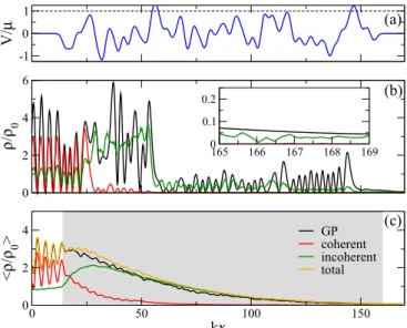
This latter observation is confirmed in the comparison of the density profiles related to Fig.3(b) which are displayed in Fig. 5 for a disorder potential length of kL=141.42.

Figure5(b)shows significantly different results predicted by the GP and tW calculations for an individual realization of the disorder. This illustrates that the mean-field description of the transport process is not valid any longer. Inspecting the inset one can furthermore infer that the GP simulation does not reach a stationary state, which is a consequence of the strong nonlinearity resulting from the atom-atom interaction, while the tW simulation attains a stationary density profile

-1 0 1

V/μ

0 2 4 6

ρ/ρ 0

0 50 100 150

kx

0 2 4

<ρ/ρ 0> ^GP_coherent

incoherent total 165 166 167 168 169 0

0.1 0.2

(a)

(b)

(c)

FIG. 5. Density profiles in the nonlocalized regime for finite interactiong=0.048μ/kand a final propagation time ofμT /= 1000. Panel (a) shows one realization of the disorder potential and panel (b) displays the corresponding density profile of an atom laser beam that propagates across this disorder potential. We can clearly see that the tW description of the transport process (red line for the coherent and green line for the incoherent part) features a breakdown of coherence and differs from the GP prediction (black line). The latter represents a “snapshot” of a nonstationary scattering process, which is reflected by the nonuniform GP density profile in the downstream region shown in the inset. Panel (c) displays the disorder average of the density profiles taking into account 1000 realizations. Despite the fact that the coherence is quickly lost within the disordered region (which is indicated by the shaded area), the disorder-averaged densities are nearly identical for both the GP and the tW method.

up to quantum fluctuations, featuring a nonnegligible part of incoherent atoms. This shows that permanently time- dependent scattering processes in the mean-field limit amount to incoherent transport in tW calculations. However, as far as the disorder-averaged density profile is concerned, we see in Fig.5(c)that the GP and tW results again coincide very well.

VI. CONCLUSIONS

In summary, we studied in this work the one-dimensional transport of Bose-Einstein condensates across disorder potentials within a guided atom laser configuration. We used the truncated Wigner method for this purpose, which was recently adapted to deal with open systems [62]. Corrections beyond the mean-field Gross-Pitaveskii description of the transport process are mainly accounted for by means of quantum noise that results from the vacuum fluctuations within the waveguide [62]. From a semiclassical point of view, the tW method corresponds to the diagonal approximation within the framework of the van Vleck–Gutzwiller approach [63].

Systematic and robust corrections beyond this diagonal approximation can arise from coherent backscattering and loop contributions [64] but do not play any role in the transport context as we argued in this paper.

(10)

As for previous studies that were based on the mean-field GP description [24,94,98], we find that Anderson localization is preserved for very weak interactions and/or short disordered regions. For stronger interaction a breakdown of AL is encountered, which is manifested by a crossover from an exponential to an algebraic∝1/Ldecrease of the transmission with the disorder length L. This crossover is accompanied by a transition from a nearly perfectly coherent flux in the Anderson localized regime to a fully incoherent flux of atoms across the disordered region in the delocalized regime. We notice that this transition is remarkably well modeled by the mean-field GP method [see Figs.3(b)and5(b)] even though the latter is not valid in the incoherent regime. Evidently, this is a consequence of the disorder average that is performed.

While an individual GP trajectory cannot correctly reproduce the many-body bosonic transport process due to the emergence of chaos in the nonstationary regime [see Fig. 5(a)], any averaging procedure removes the sensitivity of mean densities or transmissions on details of the chaotic dynamics and therefore yields rather similar results as a tW calculation that involves quantum noise.

We finally point out that the comparison between the GP and the tW method may possibly lead to more subtle conclusions in transport problems of Bose-Einstein condensates that involve more than one spatial dimension. Specifically for two-dimensional disordered systems it was shown that the presence of the nonlinearity in the GP equation may predict an inversion of the peak of coherent backscattering [99]

(which is here defined on the level of wave propagation in two spatial dimensions, and not in the Fock space of the many-body system) while a simple dephasing of the coherent backscattering peak in the presence of interaction is expected from a more microscopic point of view [36,37]. The tW method appears to be well suited to investigate this issue in more detail and to study other transport and localization phenomena of interacting bosonic matter waves in disordered systems, such as the Anderson transition in three spatial dimensions [100].

ACKNOWLEDGMENTS

We thank Klaus Richter and Juan-Diego Urbina for fruitful discussions. Financial support from Fonds de la Recherche Scientifique de Belgique (F.R.S.-FNRS) and the DFG Forschergruppe FOR760 “Scattering Systems with Com- plex Dynamics” is gratefully acknowledged. This work was also financially supported by a ULg research and mobility grant for T.E. The computational resources have been provided by the Consortium des ´Equipements de Calcul Intensif (C ´ECI), funded by the F.R.S.-FNRS under Grant No. 2.5020.11.

APPENDIX A: LOOP CONTRIBUTIONS IN CLOSED BOSE-HUBBARD SYSTEMS

In this appendix we briefly explain how to evaluate loop contributions to Eq. (43) for the specific case of a closed Bose-Hubbard system containing a finite number of Lsites and a finite number of N particles. Generally, such loop contributions originate from trajectories γ that exhibit one or several nearby encounters in phase space with themselves or their time-reversed counterpartsTγ. Provided the classical

(a) (b)

(c) (d)

(e) (f) (g)

FIG. 6. Loop contributions up to second order. For the one-leg loops [(b), (d), (f)] only one of the two possible cases of shifting one end into the encounter region is shown. Diagrams (a) and (b) are the leading order loop contributions, while the remaining ones are of next-to-leading order.

dynamics is chaotic, there exist then partner trajectories γp

that follow pieces of γ and/or Tγ and, as is illustrated in Fig. 6, switch from one piece to another one within the encounter region [69–79,101]. The overall contribution of the sum over the partner trajectories γ_p in Eq. (43) is then obtained by determining and counting all possible constructions of such partner trajectories and adding up their individual contributions [101].

We generally distinguish two-leg, one-leg, and no-leg loops, depending on how many (initial or final) ends of the trajectory lie outside the encounter regions. To evaluate their respective contributions, we follow the standard literature on Sieber-Richter pairs [71–76,79,101] where we replace the role of Planck’s constant by the effective oneeff =1/N. We furthermore have to account for the presence of an additional constant of motion besides the total energy, namely the total number of particles N. This requires performing the calculations in a reduced phase space with a fixed global phase and a fixed number of particles (see also [84]).

The contribution of two-leg loops is then given by [73,76,79]

γ_p (2ll)

exp i

Rγ ,γ_p

=

v

N(v) c

−c

d^(L^−2)(O⁻^N^enc⁾s

× c

−c

d^(L^−2)(O⁻^N^enc⁾uP(s,u,v) exp (iNs·u), (A1) where the sum runs over all partners giving rise to two-leg loops andv=(v₂,v₃, . . .) is a vector whose entries are the