make it feasible to study coherent transport of Bose-Einstein conden- sates (BEC) through various mesoscopic structures. In this work the quasi-stationary propagation of BEC matter waves through two di- mensional cavities is investigated using numerical simulations within the mean-field approach of the Gross-Pitaevskii equation.
The focus is on the interplay between interference effects and the interaction term in the non-linear wave equation. One sees that the transport properties show a complicated behaviour with multi-stabi- lity, hysteresis and dynamical instabilities for non-vanishing interac- tion. Furthermore, the prominent weak localization effect, which is a robust interference effect emerging after taking a configuration ave- rage, is reduced and partially inverted for non-vanishing interaction.“
ISBN 978-3-86845-119-1
gefördert von:
Timo Hartmann D is se rt at io n sr ei h e P hy si k - B an d 4 4
Transport of Bose-Einstein condensates through two dimensional cavities
Timo Hartmann
44
Transport of Bose-Einstein condensates through two dimensional cavities
Dissertationsreihe der Fakultät für Physik der Universität Regensburg, Band 44
Herausgegeben vom Präsidium des Alumnivereins der Physikalischen Fakultät:
Klaus Richter, Andreas Schäfer, Werner Wegscheider, Dieter Weiss
Transport of Bose-Einstein condensates through two dimensional cavities
Dissertation zur Erlangung des Doktorgrades der Naturwissenschaften (Dr. rer. nat.) der Fakultät für Physik der Universität Regensburg
vorgelegt von Timo Hartmann aus Eschwege im Juni 2014
Die Arbeit wurde von Prof. Dr. Klaus Richter angeleitet.
Das Promotionsgesuch wurde am 16.01.2012 eingereicht.
Das Promotionskolloquium fand am 05.11.2014 statt.
Prüfungsausschuss: Vorsitzender: Prof. Dr. Christian Schüller 1. Gutachter: Prof. Dr. Klaus Richter 2. Gutachter: Prof. Dr. Thomas Niehaus weiterer Prüfer: Prof. Dr. Andreas Schäfer
Transport of Bose-Einstein
condensates through two
dimensional cavities
Die Deutsche Bibliothek verzeichnet diese Publikation
in der Deutschen Nationalbibliografie. Detailierte bibliografische Daten sind im Internet über http://dnb.ddb.de abrufbar.
1. Auflage 2015
© 2015 Universitätsverlag, Regensburg Leibnizstraße 13, 93055 Regensburg Konzeption: Thomas Geiger
Umschlaggestaltung: Franz Stadler, Designcooperative Nittenau eG Layout: Timo Hartmann
Druck: Docupoint, Magdeburg ISBN: 978-3-86845-119-1
Alle Rechte vorbehalten. Ohne ausdrückliche Genehmigung des Verlags ist es nicht gestattet, dieses Buch oder Teile daraus auf fototechnischem oder elektronischem Weg zu vervielfältigen.
Weitere Informationen zum Verlagsprogramm erhalten Sie unter:
www.univerlag-regensburg.de
1 Introduction 1
2 The Bose-Einstein condensate 7
2.1 The mean-field equation for condensates . . . 7
2.1.1 Energy minimization using the Hartree ansatz . . . 7
2.1.2 The second quantization . . . 9
2.1.3 Particle-particle interaction . . . 11
2.2 External potentials for Bose-Einstein condensates . . . 12
2.2.1 Optical potentials . . . 12
2.2.2 External potentials induced by magnetic fields . . . 13
2.2.3 Restriction to two dimensions . . . 14
2.3 Gauge potentials for Bose-Einstein condensates . . . 15
2.4 Summary . . . 17
3 Stationary scattering states of the Schrödinger equation 19 3.1 Introduction . . . 19
3.2 The retarded Green function . . . 20
3.3 The tight binding model . . . 21
3.4 The tight binding model for a constant potential . . . 22
3.4.1 Eigenfunctions for a constant potential . . . 22
3.4.2 A source on an infinite lattice . . . 23
3.4.3 Calculation of the current . . . 25
3.4.4 A source in an semi-infinite strip . . . 26
3.5 The Green function in the tight binding model . . . 28
3.5.1 Handling of the left lead . . . 29
3.5.2 Calculation of the self energy . . . 30
3.5.3 Handling of the right lead . . . 32
3.6 Generalization to two dimensions . . . 33
3.6.1 The two dimensional leads . . . 34
3.6.2 Current measurement in two dimensions . . . 36
3.6.3 Magnetic gauge field . . . 36
3.6.4 Selection of the gauge field . . . 37
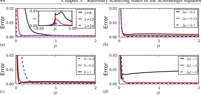
3.7 Exterior complex scaling boundary conditions . . . 38
3.7.1 Accuracy of the exterior complex scaling boundary conditions . . . 42
3.7.2 Resonances . . . 43
3.8 Scattering systems of “billiard” type . . . 47
3.8.1 B1: An almost-closed example system . . . 48
3.9 Computational complexity . . . 50
3.10 Summary, outlook and open ends . . . 52
4 Simulation of the time dependent Gross-Pitaevskii equation 53 4.1 Introduction . . . 53
4.2 Crank-Nicholson . . . 54
4.3 Incorporating the interaction term . . . 56
4.4 The Taylor series method . . . 57
4.5 The Split operator method . . . 59
4.6 Accuracy of the exterior complex scaling boundary conditions . . . 61
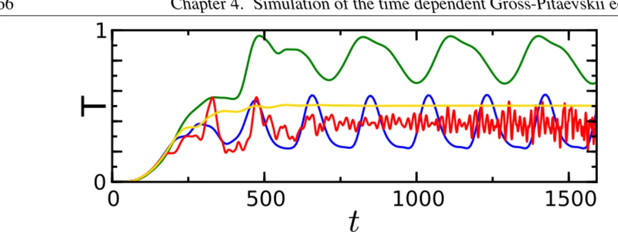
4.7 Non-adiabatic switching of the source . . . 62
5 Stationary scattering states of the Gross-Pitaevskii equation 67 5.1 Introduction . . . 67
5.1.1 Scaling behavior of the Gross-Pitaevskii equation . . . 68
5.1.2 The position dependent interaction strength . . . 69
5.2 Numerical solution of the non-linear system of equations . . . 71
5.2.1 Calculation of the derivative . . . 72
5.2.2 Selection of the start vector . . . 73
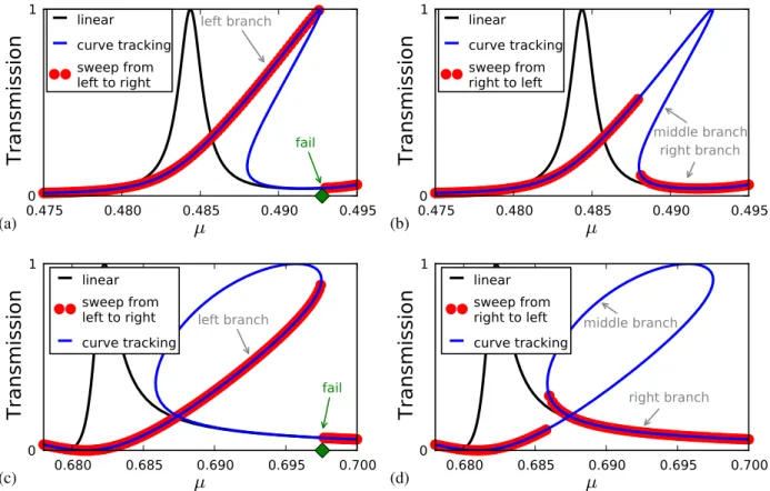
5.3 The curve tracking algorithm . . . 76
5.3.1 Calculation of the tangent vector . . . 77
5.3.2 Critical points . . . 78
5.3.3 Adaptive stepsize control . . . 81
5.3.4 Artificial homotopy . . . 82
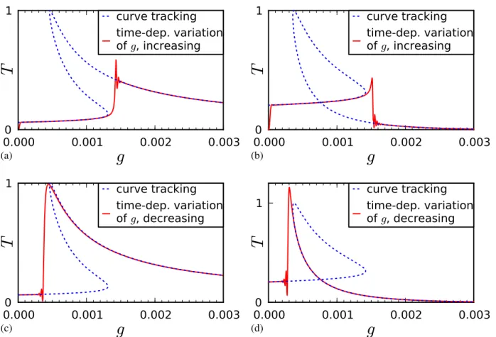
5.4 Time dependent simulations . . . 83
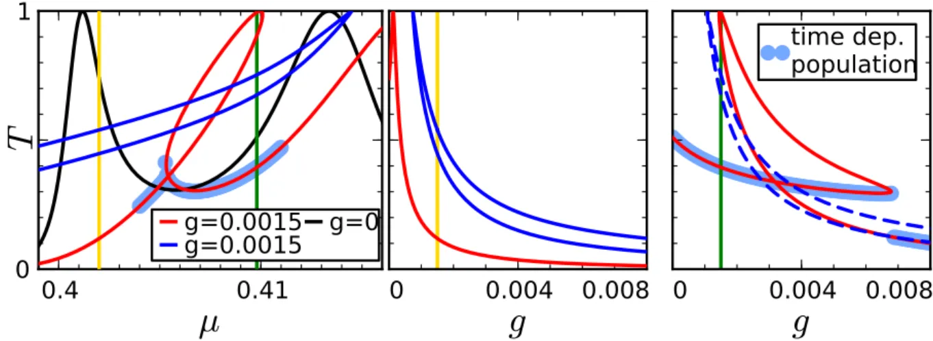
5.4.1 Time dependent population of the scattering system . . . 83
5.4.2 Time dependent variation ofµ . . . 85
5.4.3 Time dependent variation ofgandjin . . . 86
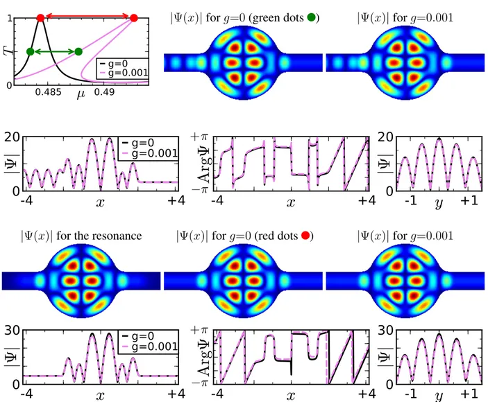
5.5 Curve tracking for various parameters . . . 88
5.6 Perturbation theory . . . 92
5.6.1 Perturbation theory for the wave function . . . 92
5.6.2 Perturbation theory for the energy . . . 94
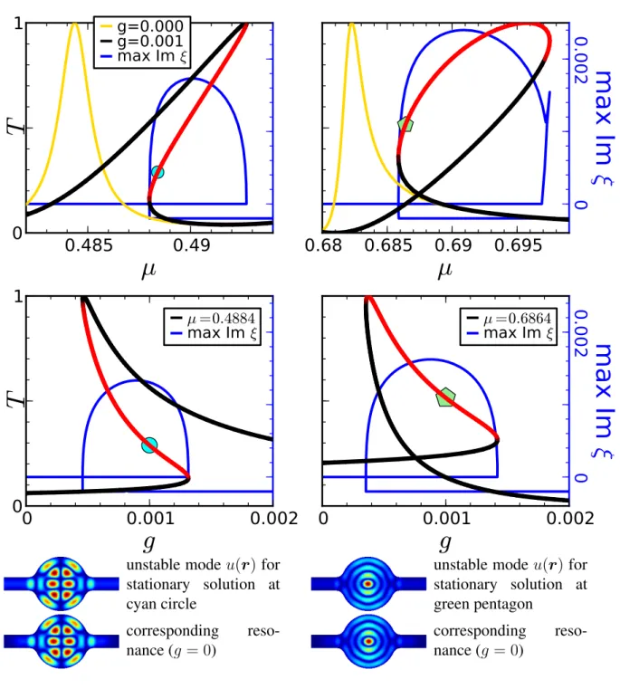
5.7 Dynamical stability . . . 100
5.8 Other geometries . . . 105
5.8.1 B2: A nearly closed system without horizontal mirror symmetry . . . 105
5.8.2 B3: A nearly closed system without any symmetry . . . 108
5.8.3 B4: Another nearly closed full symmetric system . . . 108
5.8.4 B5: A wide open system with classical chaotic dynamics . . . 113
5.9 One dimensional systems with non-trivial topology . . . 118
5.9.1 B6: A ring with vanishing potential . . . 119
5.9.2 B7: A ring with a weak disorder potential . . . 122
5.9.3 B8: A ring with a strong disorder potential . . . 122
5.10 Summary . . . 122
6 Scattering states in chaotic billiards 125
6.1 Weak localization . . . 126
6.1.1 Weak localization in the linear regime . . . 126
6.1.2 Weak localization in the non-linear regime . . . 132
6.1.3 Analysis of the classical dynamics . . . 136
6.1.4 Comparison with numerical results . . . 141
6.1.5 Direct evaluation of the semiclassical sum . . . 147
6.2 Intensity distribution . . . 150
6.2.1 Theoretical analysis . . . 150
6.2.2 Comparison with numerical results . . . 154
6.3 Other geometries . . . 157
6.3.1 B9: The clipped triangle . . . 157
6.3.2 B10: The stomach billiard . . . 157
6.3.3 B11: The half circle (narrow leads) . . . 158
6.3.4 B12: The half circle (wide leads) . . . 158
6.3.5 B13: The limaçon (narrow leads) . . . 158
6.3.6 B14: The limaçon (wide leads) . . . 158
6.4 Related effects in mesoscopic systems . . . 172
6.4.1 Coherent backscattering in disordered potentials . . . 172
6.4.2 Time-reversal mirrors in chaotic cavities . . . 173
6.4.3 Half-period Aharonov-Bohm oscillations in disordered rings . . . 174
6.5 Summary and outlook . . . 175
Appendix 177 A The Newton method 177 B The Onsager relations 180 B.1 Symmetries of the scattering matrix . . . 180
B.2 The Onsager relations . . . 183
B.3 The breakdown of the Onsager relations in the interacting case . . . 184
B.4 The generalized continuity equation . . . 185
C Transparent boundary conditions 187
D Block Gauß matrix inversion 191
E The Dyson equation 192
F Derivation of the Peierls phase 194
G The stability amplitude in Birkhoff coordinates 197
H A smooth switching function 199
References 204
List of publications
• T. Hartmann, F. Keck, H. J. Korsch and S. Mossmann. Dynamics of Bloch oscillations.
New Journal of Physics6, p. 2 (2004).
• H. J. Korsch, H.-J. Jodl and T. Hartmann.Chaos-A Programm Collection for the PC. (Springer, 2008), third edition.
• T. Hartmann, J. Michl, C. Petitjean, T. Wellens, J.-D. Urbina, K. Richter and P. Schlagheck.
Weak localization with nonlinear bosonic matter waves. Annals of Physics327, p. 1998- 2049 (2012)
• T. Hartmann, J.-D. Urbina, K. Richter and P. Schlagheck. Intensity distribution of non- linear scattering states. AIP Conference Proceedings, Volume 1468 - “Let’s Face Chaos through Nonlinear Dynamics” 8th International Summer School/Conference , p. 193 (2012), arXiv:1205.3067
Introduction
The microscopic world at the level of individual atoms behaves fundamentally different than the macroscopic world which dominates the physics we encounter in everyday life. The first is wholly described by quantum mechanics discovered in the 20th century while the latter is wholly described by classical mechanics which was already fully developed in the 19th century. In the classical world we use the Lagrange/Hamilton point particle mechanics while in the quantum world particles are described by the Schrödinger equation. The latter is essentially a classical wave equation. Albeit wave equations are ubiquitous in classical physics, the whole interpretation and conceptual foundation of the Schrödinger equation sets it apart.
While the Schrödinger wave equation has parallels in classical physics we come now to some- thing which is unknown to the classical world. A fundamentally dictum of quantum mechanics is that several particles of the same kind should be indistinguishable. The consequence of that dictum is that the description of a system consisting of many quantum particles differs drastically depending on whether one investigates several particles of the same kind or particles of several different kinds. This behavior has no counterpart in classical mechanics and underlies many interesting physical phenomena.
Another intrinsic feature of quantum particles is their spin which also lacks a classical counter- part1. The famous spin-statistic theorem [73, 162, 166] due to Fierz and Pauli relates the behavior of several indistinguishable particles to their spin. The many-particle wavefunction of several indistinguishable particles with half-integer spin (called fermions) changes the sign after an inter- change of two particle. In contrast to that the wavefunction of particles with integer spin (called bosons) remains unchanged after any permutation of particles.
Quantum effects are very susceptible to perturbations from outside which induce decoherence destroying any quantum feature. This usually means well isolated (from the environment) systems at low temperatures2 are required to observe these effects. Furthermore, at low enough temper- atures one can safely assume that the observed system is near its ground state. For a system of identical bosonic particles this ground state is particularly interesting. It is called a Bose-Einstein condensate (BEC). In contrast to fermionic systems (keyword Fermi surface), the particles in
1 The closest analogy is an intrinsic angular momentum. But the spin has several features which an intrinsic angular momentum cannot take account of.
2Low in comparison to typical excitation energies of the system.
the ground state of a many-particle bosonic system approximatively occupy all the same single particle state. For interacting particles, this results in a non-linear potential term in the effective mean field equation of motion. The influence of this non-linearity on the transport properties of a condensate will form the main topic of this thesis.
First predicted by Bose and Einstein in 1924 [25, 60, 61], it took many years to successfully create a Bose-Einstein condensate with atoms in an experiment3. The main difficulties which had to be overcome were due to the very low temperatures in the region of 10−8K . . .10−6K which are necessary to create a condensate. New techniques as trapping potentials for neutral atoms, laser cooling and evaporative cooling had to be developed. After the first success in 1995 [7, 31, 51], many other experiments with various elements have been conducted. Bose-Einstein condensates are one of the few quantum objects which can reach macroscopic dimensions and are (in principle) visible with the naked eye. In microgravity, a condensate can reach dimensions of up to several millimeters [204]. This makes them particularly interesting.
Due to the very low temperatures, the velocity of individual atoms in the condensate is quite low. Therefore the de Broglie wavelength of the atoms is very large. Additionally, measurements give very good information about the quantum state because many coherent atoms are detected simultaneously. This makes Bose-Einstein condensates an ideal system to study matter waves.
Furthermore, Bose-Einstein condensates in dilute atom gases offer a high degree of control over most experimental parameters such as external potential, particle-particle interaction and gauge potential. Therefore, condensates allow one to study many quantum effects which were originally predicted for solid state systems but are difficult to observe there due to the lack of experimental control. Examples for such effects are Bloch oscillations4 [22, 68, 95], Mott insulator transition [86, 115], Anderson localization [8, 20, 111, 115, 122, 178], weak localization in diffusive sys- tems [112] and many more. Furthermore the exceptionally good experimental control allows one to use Bose-Einstein condensates (and ultra-cold atoms in general) as model system to simulate and investigate a variety of other quantum phenomena which may be inaccessible in their native environment.
The above mentioned characteristics of Bose-Einstein condensates in dilute cold atoms make interferometry experiments with them highly sensitive to measurements of inertial forces and accelerations. This opens the road to many interesting future technical applications such as high accuracy measurements of the gravitational field for prospecting, inertial navigational systems for submerged submarines or planes (as backup for satellite navigation systems such as GPS) [55, 56]5various experimental tests of general relativity6and many more.
Anderson localization, also called strong localization, is the effect that transport (and diffu- sion) in an arbitrarily weak7 disorder potential is totally suppressed by destructive interference
3Some other effects like superfluid helium [137] or superconductivity can be considered to be due to a BEC. But these effects are somewhat “dirty” as only a tiny fraction of atoms are in the ground state [167] or quasi-particles are used. In this context fit also exciton BECs [117, 188]. There exists also a BEC made of photons [119] where the particle number is not conserved. We only consider here “real” BECs in dilute atom gases where a high fraction of particles occupy the ground state.
4The observation of Bloch oscillations in solid state systems without any “tricks” such as semiconductor super- lattices has been realized only recently as very sophisticated experimental tools are necessary [185].
5 Not all experiments to detect inertial forces use Bose-Einstein condensates. Many experiments use just cold uncondensed atoms [37, 41, 57, 80, 90].
6Such as measurement of the Lense-Thirring (also called frame-dragging) effect in earthbound table-top experi- ments, precision tests of the weak equivalence principle, detection of gravitational waves and many more [155, 204].
7The disorder strength does not matter in one and two dimensions. Of course the length scale on which the
effects. In contrast to this, the weak localization effect only causes a relatively small correction to the transport properties. It can be thought as the precursor of Anderson localization. All these localization effects are import objects of study because they are robust interference effects which are visible even after an ensemble average. They are not exclusive to quantum matter waves, but happen also for classical waves in optics and acoustics [4, 5, 115, 200]. But it is important to check if localization also happens for quantum matter waves.
Conducting systems with a random disorder potential are called diffusive. In diffusive systems, a prominent weak localization effect is coherent backscattering [3, 190]. It is the enhancement of reflection in the incident direction in comparison to other directions when a wave hits a disorder potential. In ballistic systems the disorder potential is replaced by confining the wave to a cavity with flat potential and hard wall boundaries. The shape of the cavity is chosen such that the classical motion inside the cavity is chaotic. The chaotic multiple reflection at the boundaries in ballistic system takes the role of the disorder potential in diffusive systems. In these ballistic systems, the weak localization effect is the gauge (magnetic) field dependent enhancement of reflection of matter waves for the time reversal symmetric case in comparison to broken time reversal symmetry.
In all experimental verifications of Anderson localization [20, 111, 178] and weak localization in diffusive systems [112] using BEC matter waves, the effect of particle-particle interaction is completely neglected8 9. Obviously it is of interest how well this approximation is justified.
While the localization effects depend on the linear superposition of interfering waves, the particle- particle interaction introduces a non-linearity. The crucial question is now how the non-linearity affects the interference phenomena of localization. Previous studies [98, 99] have investigated this topic for weak localization in diffusive systems or for strong localization in one-dimensional systems [159–161]. This thesis now studies the influence of the non-linearity on weak localization in two dimensional ballistic billiard systems numerically. To this end, a novel computational method to calculate stationary scattering states for non-linear wave equations will be used. The numerical results are compared to a prediction based on a semiclassical perturbation theory. The final result is that the characteristic weak localization peak shape (the reflection as function of gauge field) already known for vanishing interaction is transformed into a characteristic double peak structure for non-vanishing interaction strength [96]. Similar results are obtained for the intensity distribution of the wave function.
Experiments with Bose-Einstein condensates tend to be very complicated and take a long time to properly set them up. Both facts makes them quite expensive. Therefore a theoretical study of the possible experimental outcomes it advisable. The systems studied here are mesoscopic10 two dimensional systems. Therefore all analytic techniques11 known in one dimension to study BECs are not applicable. Neither are analytic techniques applicable which make simplifications based on the system size. The only working analytical technique is the semiclassical analysis as developed in [96]. This method is an intermediate between quantum and classical physics. The
localization happens depends on the disorder strength. In three dimensions the disorder strength has to reach a certain threshold to cause localization; this is the so-called Anderson transition.
8Either by diluting the atomic gas or by using Feshbach resonances (Sec. 2.1.3) to make the interaction strength negligible.
9Also in other technical applications (such as inertial force measurements) the non-linear interaction is often regarded as an unwanted effect which disturbs and obstructs the desired results.
10Neither very small nor very large
11These are mostly based on the solution of an ordinary second order differential equation.
quantum wave propagation is studied as perturbation (in ~) around the classical point particle dynamics while keeping the important interference effects but discarding most others. But the semiclassical analysis makes use of many universal assumptions whose validity in actual systems varies to some degree. Also many approximation are made whose error term is only qualitatively known. Therefore the semiclassical analysis has to be checked with numerical simulations12. This thesis fulfills the role of checking the semiclassical prediction for the weak localization effect and shows possible outcomes of future experiments.
Successful experiments with degenerate quantum gases have studied the Anderson localization in one [20, 178] and three dimensions [111, 122]13, the Bloch oscillation [68], the Mott insulator transition [86], and many other basic quantum effects. Also weak localization in diffusive systems (manifest as coherent backscattering in momentum space) has been observed for a quasi two dimensional Bose-Einstein condensate in a disordered potential [112]. But no experiment has studied the effect of interaction on localization thus far. But the steady progress in experimental sophistication leads to hope that experiments to study the effect of atom-atom interaction on localization (of course from perspective of this work especially on weak localization in ballistic systems) will be possible in the near future. Examples of the necessary experimental repertoire are a guided atom laser [45, 88] (a source for “monochromatic” atoms with a well defined incoming velocity), almost arbitrarily shaped potentials for cold atoms [28, 78, 101, 105, 116, 148] and artificial gauge fields [49, 136]. The building blocks for successful experimental tests of the results of this thesis do exist; all it remains is to put them together.
Outline
The first three chapters (Chap. 2-4) provide the (more or less) well known technical foundations to simulate Bose-Einstein condensates on the basis of the mean-field description. These chapters can be skipped by readers not interested in known technical details. In the last two chapters (Chap. 5-6) a novel way to calculate stationary scattering of the Gross-Pitaevskii equation is used to investigate how the weak localization effect in ballistic billiard systems is modified by the non- linear particle-particle interaction. Readers interested in technical details should focus on Chap. 5 while Chap. 6 contains the “real physics”.
Chap. 2 provides a short overview of the mean field description of Bose-Einstein condensates and discusses how to generate artificial external and gauge potentials for neutral atoms. The final result of this chapter is the two-dimensional Gross-Pitaevskii equation (2.17) which is used in the rest of this work.
Chap. 3 is a technical introduction to the tight binding model for the linear Schrödinger equa- tion. This model allows one to calculate stationary scattering states of a two dimensional cavity with several infinite leads attached. This is done by solving linear systems of equations and forms the foundation to investigate scattering states of the non-linear Gross-Pitaevskii equation in Chap. 5. In the tight binding model leads are incorporated using self energies. Alternative boundary conditions in the form of exterior complex scaling are also developed. These are useful to handle the leads in time dependent simulations and for the dynamical stability analysis.
Chap. 4 is a technical discussion of several methods to simulate the time propagation of the Gross-Pitaevskii equation. Each method has its advantages and disadvantages.
12Actually, the numerical data was available before the semiclassical analysis was completed. This data was used to determine several terms appearing in the semiclassical results.
13[122] uses an ultracold Fermi gas instead of a BEC.
Chap. 5 introduces a novel way to calculate stationary scattering states of the two dimensional Gross-Pitaevskii equation. The non-linearity of this equation makes this a non-trivial and hard task but also provides interesting effects (like multi-stability, hysteresis and instabilities) not exist- ing in linear systems. Technically the scattering states are calculated by solving a non-linear sys- tem of equations. The dynamical stability of such found stationary states is investigated using the Bogoliubov-de Gennes equation. The time-independent ansatz is compared with time-dependent simulations and a perturbative ansatz.
Chap. 6 focuses on universal transport behavior in the form of the weak localization effect which does not depend on the details of the investigated system as long as it belongs to a specific universality class. The methods discussed in the previous chapters are used to analyze how the weak localization effect in ballistic systems is modified by the particle-particle interaction. The numerical results are compared to a semiclassical theory. Furthermore the intensity distribution of the wave function is studied in a similar way. Related effects in other systems are also briefly discussed.
The appendix supplements the previous chapters with various technical details. App. A gives a short introduction into the Newton method to solve non-linear equations. App. B derives the On- sager relations which seem to be common knowledge but whose derivation is hardly found in the literature. App. C describes the “perfect” transparent boundary conditions for time simulations.
App. D and App. E emphasize the technical details for the self energy calculation in the tight- binding model. App. F provides a more systematic approach to the Peierls phase which is usually introduced in some ad hoc manner. App. G calculates the semiclassical stability amplitude for ballistic two dimensional billiard systems. App. H analyzes a switching function.
The Bose-Einstein condensate
This chapter provides a short overview of the mathematical description of Bose-Einstein con- densates and of the possibilities to manipulate these condensates experimentally. The theory presented here is based on the assumption that we want to describe bosonic atoms in dilute gases.
For experimental investigations of Bose-Einstein condensates, the alkali metals are of particular interest because of the multitude of strong spectral lines they provide which allow for manipu- lation (cooling and trapping) of these atoms by lasers. But other elements are possible to use, too. Successful Bose-Einstein condensation has been demonstrated using the atoms1H,7Li,23Na,
39K,41K,52Cr,85Rb,87Rb,133Cs,170Yb,174Yb,4He∗,168Erand a few others.
2.1 The mean-field equation for condensates
In this section we derive the mean-field description of Bose-Einstein condensates at zero temper- ature. The resulting equation of motion is called the Gross-Pitaevskii equation. There are many methods leading to this result and two of them are described here. The material covered here can be found in many standard references [48, 129, 167, 169].
2.1.1 Energy minimization using the Hartree ansatz
In conventional quantum mechanics a system of N identical bosonic particles is described by a wave function Ψ(r1, . . . ,rN) which is symmetric under any permutation of particles. The corresponding Hamilton operator can be written as [167]:
H =
N
X
j=1
"
− ~2
2m∆j+V(rj)
#
+ X
1≤j<k≤N
U(rj−rk). (2.1) It acts on the space of all square integrable functionsR3N →Cwhich are invariant under permu- tations of arbitrary coordinates.
Here V(r) is an external potential which for example can be produced by the methods of Sec. 2.2. U(rj−rk)is the two-body interaction potential which will be explained in more detail in Sec. 2.1.3. We are working in a dilute gas regime where the probability that three or more
particles collide is negligible; therefore three and more body interactions are neglected. They are unwanted anyway because they lead to the loss of particles from the condensate [167, 206].
The ground state ofH can be found by minimizing the total energy E[Ψ] =
Z
Ψ(r1,r2, . . . ,rN)∗HΨ(r1,r2, . . . ,rN)
N
Y
j=1
drj under the normalization constraintR |Ψ(r1,r2, . . . ,rN)|2QNj=1drj = 1.
The Hilbert space of total symmetric functions in N variables is extremely large. Therefore we must restrict ourselves to a small portion of it. Particularly we construct the many body wave function as a simple product state of identical single particle states. This is called a Hartree ansatz:
Ψ(r1,r2, . . . ,rN) =
N
Y
j=1
φ(rj). (2.2)
Hereφ(r)∈ L(R3)is a normalized single particle wave function (R |φ(r)|2dr= 1).
Inserting the Hartree ansatz into the energy functional gives E[φ] =
Z
Ψ(r1,r2, . . . ,rN)∗HΨ(r1,r2, . . . ,rN)
N
Y
j=1
drj
=N
Z "
~
2m|∇φ(r)|2+V(r)|φ(r)|2
#
+N(N −1) 2
Z
U(r−r0)|φ(r)|2|φ(r0)|2drdr0 . It is more convenient to choose another normalization. The replacementψ(r) =√
N φ(r)allows us to move the particle numberN out of the energy functional into the normalization condition
R |ψ(r)|2dr=N by using N−1N ≈1valid for largeN. E[ψ] =
Z "
~
2m |∇ψ(r)|2 +V(r)|ψ(r)|2
#
+1 2
Z
U(r−r0)|ψ(r)|2|ψ(r0)|2drdr0 . (2.3) The approximate ground state of the many particle Hamiltonian Eq. (2.2) can now be found using a variational principle. We demand that ψ(r) minimizes the energy functional Eq. (2.3) under the normalization constraint that the particle number is fixed. Using a Lagrange multiplier µto handle the constraint we arrive at
δE−µδN = 0 (2.4)
This equation for the variation has to be fulfilled with respect to the independent variation ofψ(r) and its complex conjugateψ∗(r). Finally the Euler-Lagrange equation for Eq. (2.4) gives us the (generalized) Gross-Pitaevskii equation [159, 167]
µ ψ(r) =
"
−~2
2m∆ +V(r) +
Z
U(r−r0)|ψ(r0)|2
#
ψ(r) (2.5)
which is a mean-field equation describing approximatively the many particle physics. In this context µ is called the chemical potential. It describes the energy necessary to add one more particle to the system. ψ(r)is called the condensate wave function.
The (approximative) time evolution of the many particle system Eq. (2.1) can also be derived using a variational approach [48, 169]:
δ
"
−i~
Z
ψ∗(r, t)∂
∂tψ(r, t)drdt+
Z
E[ψ]dt
#
= 0. (2.6)
In this ansatz we have introduced a time dependence into ψ. The Euler-Lagrange equations for Eq. (2.6) gives us the time dependent (generalized) Gross-Pitaevskii equation:
i~
∂ψ(r, t)
∂t =
"
−~2
2m∆ +V(r) +
Z
U(r−r0)|ψ(r0, t)|2
#
ψ(r, t). (2.7)
The mathematical rigorous results
In order to find the true ground state of the Hamiltonian Eq. (2.1) the minimization has to be done with respect to the whole set of symmetrical many particle wave functions which is much larger then the set of simple product states of the form Eq. (2.2). There exists rigorous mathematical proofs [132–134] that for a δ-interaction U(r) = aδ(r)(see Sec. 2.1.3) in the limit N → ∞ anda0 =N a =fixed, the ground state many-particle wave function and the ground state energy converge in some well defined sense to the solution of the stationary Gross-Pitaevskii equation in the form of Eq. (2.5). The time dependent variant Eq. (2.7) can also be recovered [64, 168].
2.1.2 The second quantization
While in Sec. 2.1.1 we used conventional quantum mechanics to derive a mean-field approxima- tion of the many particle dynamics there is another approach which uses the framework of second quantization [154, 156, 186]. This framework provides a better connection to quantum statistical mechanics which allows some insight into the process of condensation. Furthermore one can go beyond the mean-field approximation.
The Hamilton operator in second quantization can be written as:
Hˆ =
Z
dr Ψˆ†(r) −~2
2m∆ +V(r)
!
Ψ(r)ˆ + 1
2
Z
drdr0 Ψˆ†(r) ˆΨ†(r0)U(r−r0) ˆΨ(r0) ˆΨ(r).
(2.8)
This is a generalization of Eq. (2.1). Here the Ψˆ†(r) and Ψ(r)ˆ are the bosonic creation and annihilation operators in the position basis which in this representation are traditionally called field operators. Their physical interpretation is thatΨˆ†(r)creates a particle at positionrand that Ψ(r)ˆ annihilates a particle at the same position.
Working in the Heisenberg picture we get the following equation of motion for the field oper- ator:
i~∂
∂t
Ψ(r, t) =ˆ hΨ,ˆ Hˆi
=
"
− ~2
2m∆ +V(r) +
Z
dr0Ψˆ†(r0, t)U(r−r0) ˆΨ(r0, t)
#
Ψ(r, t)ˆ .
(2.9)
The field operators are now rewritten in an orthonormal basis {uj(r)}∞j=0 of the single particle Hilbert space:
Ψ(r) =ˆ u0(r)ˆa0+
∞
X
j=1
uj(r)ˆaj . (2.10)
Here the creation and annihilationaˆ†j,ˆaj operators operate on Fock space in the usual way ˆ
a†j|n0, n1, . . . , nj, . . .i=qnj+ 1 |n0, n1, . . . , nj+ 1, . . .i ˆ
aj|n0, n1, . . . , nj, . . .i=√
nj |n0, n1, . . . , nj −1, . . .i (2.11) and obey the usual bosonic commutation relations
hˆai,aˆ†ji=δi,j hˆa†i,aˆ†ji= 0 haˆi,ˆaji= 0 . (2.12) In a Bose-Einstein condensate the ground stateu0(r)is assumed to be macroscopically occupied while the number of particles in the higher states is assumed to be negligible.
Comparing the expectation value of the particle number in the ground state N =Dˆa†0ˆa0E
with the expectation value of the commutation relation 1 =Dhaˆ0,ˆa†0iE
we see that the latter is suppressed by a factor of N1. BecauseN is assumed to be macroscopically large we can make the approximationhˆa0,ˆa†0i≈0and treat the creation and annihilation operator for the ground state like c-numbers [48]. This is analogous to the transition from quantum to classical mechanics. Using the replacementˆa0 = ˆa†0 =√
N we can write the field operator as1 Ψ(r) =ˆ √
N u0(r) +
∞
X
j=1
uj(r)ˆaj =√
N u0(r) +δΨ(r)ˆ .
HereδΨ(r)ˆ is a field operator acting only on the higher modes whose occupation is negligible compared to the ground mode: DδΨ(r)ˆ E≈0.
Adding a time dependence gives the Bogoliubov ansatz [71, 72] where one defines a (c- number) wave functionψdescribing the condensate as the expectation value of the field operator
ψ(r, t) =DΨ(r, t)ˆ E and decomposes the field operator according to
Ψ(r, t) =ˆ ψ(r, t) +δΨ(r, t)ˆ .
Neglecting the termδΨ(r, t)ˆ which describes the non-condensed atoms and inserting this Bogo- liubov ansatz into the Heisenberg equations of motion Eq. (2.9) we arrive at the usual (general- ized) Gross-Pitaevskii equation (2.7)
i~
∂ψ(r, t)
∂t =
"
−~2
2m∆ +V(r) +
Z
U(r−r0)|ψ(r0, t)|2
#
ψ(r, t).
1A complex phase ofˆa0can be absorbed into the definition ofu0.
A crucial point concerning the Bogoliubov ansatz is that the system is not allowed to be in a pure number state like in Sec. 2.1.1. Otherwise the expectation value ofΨˆ would be zero. Therefore one works with a grand canonical ensemble and introduces an infinitely small artificial term which breaks the conservation of the particle number in order to get a non-vanishing expectation value for the field operator [211]. This is similar to the scenario of a spontaneously broken symmetry.
A closely related ansatz is the assumption that the condensate is described by a coherent state [9, 16, 43, 210]. For a rigorous mathematical analysis why it is allowed to replaceˆa0 andˆa†0with c-numbers and why the Bogoliubov ansatz works see the references [81, 133].
On the other hand, the fact that nature realizes a superselection rule forbidding superpositions of states with different atom numbers casts some doubt on the Bogoliubov ansatz [128]. There are some proposals to avoid the explicit symmetry breaking [39]. But in the end all approaches should give the same result in the thermodynamic limit.
The second quantization allows one to go beyond the mean-field approximation. To this end we take the expectation value of Eq. (2.9). The mean-field theory arises by replacing the expectation value of the product of field operators by a product of expectation values:
DΨˆ†(r0, t) ˆΨ(r0, t) ˆΨ(r, t)E≈DΨˆ†(r0, t)E DΨ(rˆ 0, t)E DΨ(rˆ 0, t)E .
Using cumulants one can systematically improve this approximation and go beyond the mean- field theory to describe the condensate [87, 120]. In this framework one can for example investi- gate the depletion of the condensate [67] and investigate the validity of the mean-field equation.
2.1.3 Particle-particle interaction
The scattering of two particles with the interaction potentialU(rj −rk) can be analyzed using a partial wave ansatz [154, 187, 198]. At very low energies one can show that s-wave scattering alone is sufficient to describe the scattering process [129, 167]. The p-wave scattering is for- bidden because of the bosonic symmetry while higher angular momentum terms are kinetically suppressed. Therefore it is justified to approximate the interaction by a simple contact potential:
U(rj−rk) = 4π~2as
m δ(rj−rk). (2.13)
Here the scattering lengthasis a parameter which depends on the type of atoms we are using.
The scattering length as can be changed by Feshbach resonances [44, 121, 167]. The inter- atomic potential depends on the electronic spin configuration. In a Feshbach scenario the scatter- ing energyEscatterof the normal configuration gets in resonance with the energyEboundof a bound state in another configuration. See Fig. 2.1 for an illustration. Second order perturbation theory gives us [167]:
4π~2as
m = 4π~2as,0
m +|hψbound|Hcoupling|ψscatteri|2 Escatter−Ebound .
If the magnetic moments of the two states are different the value of Escatter−Ebounddepends on the external magnetic field. This way we can control the scattering lengthasand even setas to zero by carefully tuning the magnetic field.
Figure 2.1: The situation in a Feshbach resonance scenario. The black potential arises in one electronic spin configuration, the blue potential arises from an- other electronic spin configuration. The blue po- tential curve allows several bound states colored in red. The energy difference between the two poten- tials can be controlled by applying an external mag- netic field.
Inserting the approximation Eq. (2.13) into Eq. (2.5) and Eq. (2.7) we get the following sta- tionary and time dependent (three-dimensional) Gross-Pitaevskii equation
µ ψ(r) =
"
−~2
2m∆ +V(r) +U0|ψ(r)|2
#
ψ(r) i~∂ψ(r, t)
∂t =
"
−~2
2m∆ +V(r) +U0|ψ(r, t)|2
#
ψ(r, t)
(2.14)
withU0 = 4π~2as/m. These equations are only valid in the dilute gas regime where the condition na3s 1(herenis the particle density) is satisfied [48].
2.2 External potentials for Bose-Einstein condensates
There are basically three ways to create external potentials for neutral atoms: One can use grav- itational2, electrical or magnetical fields. Here we discuss the latter two. The external potential based on electrical fields uses the AC Stark effect at optical frequencies. The external potential based on magnetic fields makes use of the Zeeman effect. The presentation given here is based on [48, 129, 167, 169].
2.2.1 Optical potentials
An electrical fieldEinduces an electrical dipole momentp=αEin a neutral atom. Hereαis the polarizability. This dipole moment interacts with the electrical field; the value of the interaction energy is Vpot = −R0Ep·dE = −12α|E|2. That is the quadratic Stark effect. The DC Stark effect is related to static electric fields while the AC Stark effect is related to electrical fields of electromagnetic waves.
The AC Stark effect is a nice way to generate external potentials for neutral atoms. One uses electromagnetic waves (generated by lasers) with frequencyωin the vicinity of an atomic transi- tion between two states, say ground state|giand excited state|ei. The polarizabilityαcan then be calculated in second order perturbation theory as [167]
α= Re |he|d·E/|E||gi|2 Ee−Eg −~ω−i~Γe/2 .
2The gravitational field of the earth is not always wanted in experiments; hence there exists Bose Einstein con- densate experiments which use microgravity in falltowers [204].
Figure 2.2: Magnetic moments which are an- tiparallel to an applied magnetic fieldB are at- tracted to regions where B = |B| is minimal.
Parallel aligned magnetic moments are attracted to regions whereBis larger.
Heredis the electrical dipole operator andΓ−1e is the lifetime of the excited state|ei. The external potential for the neutral atoms is then
Vpot=−1
2 α D|E|2E
time averaged .
The sign of the interaction energyVpotdepends on the detuning of the frequencyωwith respect to the transition frequency. Furthermore the magnitude of the interaction energyVpotdepends on the intensity of the electromagnetic wave. It follows that blue detuned lasers generate a repulsive potential ejecting atoms from high intensity regions. Red detuned lasers generate an attractive potential capturing atoms inside high intensity regions. The latter effect is also used in optical tweezers (operating not on atoms but on (literally) microscopical particles).
A position dependent external potential Vpot(r) can be created by varying the intensity of the laser beam with the position r. This provides many ways to craft almost arbitrary external potentials for neutral atoms. The simplest example is that the beam of a red detuned (hence attractive) laser itself is used as a quasi-onedimensional waveguide [45, 88] which may be called a
“guided atom laser”. As the ultracold atoms move very slowly a fast moving laser beam (deflected by acousto-optic modulators) can be used to inscribe potential landscapes on the condensate [78, 101, 105, 116, 148]. Spatial light modulators [28] can be used, too. Disordered potentials can be created using speckle patterns [3, 182].
Two counterpropagating laser beams create standing wave whose intensity varies on the scale of half a wavelength. If one uses red detuned lasers this allows one to confine a condensate to a two dimensional plane. This will be discussed in more detail in Sec. 2.2.3. Various other lattice potentials can also be created using standing waves with (two or more) laser beams in many different configurations [182].
2.2.2 External potentials induced by magnetic fields
The energy level of an atom with non-vanishing total angular momentum F split into 2F + 1 hyperfine states mF = −F,−F + 1, . . . ,+F by applying a magnetic fieldB. This is called the Zeeman effect. For small magnetic fields B the energy shift for each of the hyperfine states is given by [93, 167]
Vpot =−gFµBBmF .
HeregF is the Landé factor andµBis the Bohr magneton. The sign ofgF can be both positive or negative.
In an inhomogeneous magnetic field, magnetic dipoles experience a force. Atoms whose mag- netic moment gFmF points in the same direction as the magnetic field B (i.e. gFmF>0) are attracted to regions where B = |B| is large. These atoms are called high field seekers. Atoms whose magnetic moment gFmF points in the opposite direction as the magnetic field B (i.e.
gFmF<0) are attracted to regions where B = |B| is small. These atoms are called low field seekers. See Fig. 2.2 for an illustration. A position dependent modulus of the magnetic field can thus be used to create external potentials for neutral atoms with a non-vanishing magnetic momentmF.
While a local maximum ofB =|B|cannot exist in a current free region, a local minimum3can be created. The minimum ofB should not be zero because then the atoms loose their orientation.
Typical experimental realizations as the Ioffe-Pritchard trap [167] use two or more superimposed magnetic fields to create such minima. Advanced designs for magnetic traps are so small that they fit on microelectronic chips [21, 35, 108].
2.2.3 Restriction to two dimensions
In this work we want to investigate the quantum transport properties of two-dimensional Bose Einstein condensates. To this end the motion in one dimension, say the z-direction, has to be restricted. Experimentally this can be done for example with a standing wave created by two counterpropagating red detuned lasers as described in Sec. 2.2.1. The following discussion is based on [98].
To investigate the restriction to two dimensions theoretically we assume a harmonic confine- mentV⊥(z) = 12mw2⊥z2 inz-direction. The confinement has to be strong enough that the differ- ence between ground state and first excited state inz-direction exceeds all other relevant energy scales (for example the kinetic energy inx, y-direction and the interaction energy) of the system.
Furthermore we assume that the potential inx, y-direction varies on a much larger scale than in z-direction. Under these conditions the condensate is always in the ground state inz-direction.
This justifies a separation ansatz
Ψ(x, y, z, t) = ψ(x, y, t)φ(z)
where φ(z) is a function which depends predominately on z and only weakly on x, y, t (i.e.
∂φ
∂x∼=0,∂φ∂y∼=0,∂φ∂t∼=0). The normalization R |φ(z)|2dz=1 is chosen. This ansatz inserted into the three dimensional Gross-Pitaevskii equation (2.14) gives
φ(z)i~∂ψ(x, y, t)
∂t =φ(z)
"
− ~2 2m
∂2
∂x2 + ∂2
∂y2
!
+ ˜V(x, y)
#
ψ(x, y, t) +ψ(x, y, t)
"
−~2 2m
∂2
∂z2 +V⊥(z) +U0|ψ(x, y, t)|2|φ(z)|2
#
φ(z).
(2.15)
The (non-linear) equation for the ground state inz direction reads µ⊥φ(z) =
"
−~2 2m
∂2
∂z2 +V⊥(z) +U0|ψ(x, y, t)|2|φ(z)|2
#
φ(z).
3 This has to be contrasted with the maximum principle [77] for the individual components ofB which are disallowed to have either local minima or maxima in current free regions.
For small interaction strengths U0 this equation can be solved perturbatively using the non- interacting ground state wave function [154]
φ0(z) = (√
πa⊥)−1/2 e−x2/(2a2⊥) with the harmonic oscillator lengtha⊥ =q~/(mw⊥). This gives
µ⊥ = 12~ω⊥+U0|ψ(x, y, t)|2Dφ0|φ0|2φ0E= 12~ω⊥+~2 m
√ 8πas
a⊥
|ψ(x, y, t)|2
where we have used U0 = 4π~2as/m. Inserting this result into Eq. (2.14) gives the two dimen- sional Gross-Pitaevskii equation
i~
∂ψ(x, y, t)
∂t =
"
−~2 2m
∂2
∂x2 + ∂2
∂y2
!
+V(x, y) +g~2
m|ψ(x, y, t)|2
#
ψ(x, y, t) withg =√
8π as/a⊥ andV(x, y) = ˜V(x, y) + 12~w⊥.
The theoretical discussion remains valid if we introduce an adiabatically slow position depen- dence (in x, y-direction) of the harmonic confinement potential in z-direction. This makes a⊥
depend onx, yand thus leads to a position dependent interaction strengthg(x, y).
In summary one can say that the restriction to two dimensions leads to a renormalization of the interaction strength but does not change the form of the Gross-Pitaevskii equation.
2.3 Gauge potentials for Bose-Einstein condensates
In experiments one usually uses uncharged particles whose center-of-mass motion is not affected by magnetic gauge fields4 to create Bose Einstein condensates. Consequently there is no gauge potential in the mean field time evolution equation (2.14). But using internal states one can simulate magnetic fields by creating artificial gauge potentials. This section describes how this is done. The presentation is based on [49].
Let|ai,|c1i,|c2i, . . . ,|cNibe a position-dependent orthonormal basis for the N + 1internal states. It is assumed that the basis changes adiabatically slowly with respect to the position. In this case one can assume that the particles stay in one internal state, say|ai, for all relevant positions and times. The contribution from all other internal states |c1i, . . . ,|cNi can be neglected. The total wave function|Ψi=ψ|ai+{terms withc}can therefore be approximated by|Ψi=ψ|ai.
We must now transform the time evolution equation for|Ψiin one forψ. For sake of simplicity we neglect the atom-atom interactions and external potentials. The time evolution for|Ψiis then given by
i~∂
∂t |Ψi= 1
2m [−i~∇]2 |Ψi . (2.16)
The action of∇2on|Ψiis given by
∇|Ψi= (∇ψ)|ai+ψ|∇ai
∇2|Ψi= (∆ψ)|ai+ 2(∇ψ)· |∇ai+ψ|∆ai .
4Of course magnetic fields can be used to create external potentials as described in Sec. 2.2.2 or to manipulate internal states of the atoms.
Figure 2.3: This figure shows aΛ-configuration as used in STIRAP. Three internal states|1i,|2i,|3iare coupled by two laser beamsL13, L23with a finite detuning.
Projecting Eq. (2.16) onto|aiand usingψ =ha|Ψiwe arrive at i~∂
∂t ψ =−~2
2m [∆ + 2ha|∇ai ·∇+ha|∆ai] ψ . Comparing this with
1
2m[−i~∇−qA]2 =−~2
2m∆ + q2
2mA2+i~q
2m[∇·A] +i~q mA·∇
we see that the artificial gauge potentialA(with the artificial chargeq) must be given by A=i~
qha|∇ai . Furthermore it follows that the time evolution equation forψ
i~
∂
∂t ψ = 1
2m[−i~∇−qA]2 ψ+W ψ must contain a further potential termW(r)given by
2m
~2
W =− ha|∆ai+ha|∇ai · ha|∇ai+∇· ha|∇ai
=ha|∇ai · ha|∇ai+h∇a·|∇ai .
The term W(r) can be rewritten by using orthonormality and completeness 1 = |ai ha| +
PN
n=1|cni hcn|of the internal basis states as 2m
~2 W =
N
X
n=1
Cn·C∗n
with (also noteha|∇ai=− h∇a|ai)
Cn =ha|∇cni=− h∇a|cni C∗n =h∇cn|ai=− hcn|∇ai .
A possible physical realization[49, 114] of this scheme to create artificial gauge potentials uses aΛ-type internal level structure (see Fig. 2.3) as is used in STIRAP (stimulated Raman adiabatic passage)[17]. Two laser beams L13, L23 couple the three internal states |1i,|2i,|3i into three dressed states: a dark state |Di and two bright states |B+i,|B−i. The dark state |Didoes not contain the excited state |3i and is therefore longlived. This would correspond to our|ai. The coupling depends on the amplitude (this means modulus and phase) of the electric field of the laser beams and on the detuning. Therefore the creation of artificial gauge potentials works best if the photons of one of the lasers have orbital angular momentum [114] as then the phase of the electric
Figure 2.4: A trap containing a reservoir of atoms in a Bose-Einstein condensate is cou- pled to a waveguide. Inside the waveguide the atoms propagate as a plane wave. The waveguide itself is connected to a scatter- ing region. As we are interested in trans- port properties, we measure reflection and transmission through the scattering region.
field is strongly position dependent. Other experimental realizations [49, 135, 136] use a spatial modulation of the intensity and/or detuning of the lasers. Using variations of these approaches allows one to simulate other kind of gauge potentials as for example spin-orbit interaction.
In summary one can say that artificial gauge potentials can be created as some kind of Berry phase. ConsequentlyA=i~ha|∇ai/qis called a Berry-Mead connection. The potentialW(r) has to be combined with the potentials created by the methods of Sec. 2.2 to create the final potentialV(r).
2.4 Summary
In the rest of this work we use the inhomogeneous two-dimensional Gross-Pitaevskii equation i~∂
∂tΨ(r, t) =HΨ(r, t) +g(r)~2
m|Ψ(r, t)|2Ψ(r, t) +S(r)e−iµt/~ with H = 1
2m[−i~∇−qA(r)]2+V(r)
(2.17)
with position r=(x, y), time independent Hamilton operator H, gauge potential A(r) (with charge q), external potential V(r) and (dimensionless) position dependent interaction strength g(r). This equation of motion is obtained by combining Sec. 2.1, Sec. 2.2 and Sec. 2.3 and describes a Bose-Einstein condensate restricted to two dimensions.
The interaction strengthg(r)can be controlled by using Feshbach resonances (see Sec. 2.1.3), by changing the transversal confinement (see Sec. 2.2.3) or by modifying the overall particle density (see Sec. 5.1.1). The gauge potential A(r)corresponds to a simulated5 magnetic field B(r) =∇×A(r).
So far, the only term unaccounted for is the inhomogeneous source term S(r)e−iµt/~. This source term models a particle reservoir which injects particles into our system as illustrated in Sec. 3.4.2 and Sec. 4.7. The physical picture is that one couples a trap containing a Bose-Einstein condensate (with chemical potential µ) to a waveguide (see Fig. 2.4). Inside the waveguide the atoms propagate as plane waves. The waveguide (and scattering potential) is modelled by H while the effect of the coupled condensate in the trap is described by the source term. A possible realization could be a condensate in a magnetic trap with a red detuned (i.e. attractive) laser beam as a waveguide. The coupling would be accomplished by using microwave radiation to change the magnetic moment of the atoms to zero. Then the atoms are not affected by the trapping potential anymore and propagate inside the waveguide. This setup is called a guided atom laser [45, 67, 88].
5Not to be confused with the real magnetic field trapping potentials used in Sec. 2.2.2.
In this work we are studying open scattering systems. The HamiltonianHdescribes two semi- infinite leads connected by a scattering region. The reflection and transmission through the scat- tering region are measured (see Fig. 2.4).
Non-linear Schrödinger equations such as Eq. (2.17) (without gauge potential) also arise in other contexts such as non-linear optics [27] and water waves in shallow waters [212].