Iron Speciation in Fram Strait and Over the Northeast Greenland Shelf:

doi: 10.3389/fmars.2020.609379

Edited by:

Christel Hassler, Université de Genève, Switzerland Reviewed by:

Dario Omanovic, Rudjer Boskovic Institute, Croatia Dawei Pan, Yantai Institute of Coastal Zone Research (CAS), China

*Correspondence:

Indah Ardiningsih indah.ardiningsih@nioz.nl

Specialty section:

This article was submitted to Marine Biogeochemistry, a section of the journal Frontiers in Marine Science

Received:23 September 2020 Accepted:14 December 2020 Published:21 January 2021

Citation:

Ardiningsih I, Zhu K, Lodeiro P, Gledhill M, Reichart G-J, Achterberg EP, Middag R and Gerringa LJA (2021) Iron Speciation in Fram Strait and Over the Northeast Greenland Shelf: An Inter-Comparison Study of Voltammetric Methods.

Front. Mar. Sci. 7:609379.

doi: 10.3389/fmars.2020.609379

Iron Speciation in Fram Strait and Over the Northeast Greenland Shelf:

An Inter-Comparison Study of Voltammetric Methods

Indah Ardiningsih¹* , Kechen Zhu², Pablo Lodeiro², Martha Gledhill²,

Gert-Jan Reichart^1,3, Eric P. Achterberg², Rob Middag¹and Loes J. A. Gerringa¹

1Department of Ocean Systems, Royal Netherlands Institute for Sea Research (NIOZ), Texel, Netherlands,²GEOMAR Helmholtz Centre for Ocean Research, Kiel, Germany,³Department of Earth Sciences, Faculty of Geosciences, University of Utrecht, Utrecht, Netherlands

Competitive ligand exchange – adsorptive cathodic stripping voltammetry (CLE-AdCSV) is a widely used technique to determine dissolved iron (Fe) speciation in seawater, and involves competition for Fe of a known added ligand (AL) with natural organic ligands. Three different ALs were used, 2-(2-thiazolylazo)-p-cresol (TAC), salicylaldoxime (SA) and 1-nitroso-2-napthol (NN). The total ligand concentrations ([Lt]) and conditional stability constants (log K⁰Fe⁰L) obtained using the different ALs are compared. The comparison was done on seawater samples from Fram Strait and northeast Greenland shelf region, including the Norske Trough, Nioghalvfjerdsfjorden (79N) Glacier front and Westwind Trough. Data interpretation using a one-ligand model resulted in [Lt]SA

(2.72±0.99 nM eq Fe)>[Lt]TAC(1.77±0.57 nM eq Fe)>[Lt]NN(1.57±0.58 nM eq Fe); with the mean of logK⁰Fe⁰Lbeing the highest for TAC (log⁰KFe⁰L(TAC)= 12.8±0.5), followed by SA (log K⁰_Fe⁰_L(SA) = 10.9 ± 0.4) and NN (log K⁰_Fe⁰_L(NN) = 10.1 ± 0.6).

These differences are only partly explained by the detection windows employed, and are probably due to uncertainties propagated from the calibration and the heterogeneity of the natural organic ligands. An almost constant ratio of [Lt]_TAC/[Lt]_SA= 0.5 – 0.6 was obtained in samples over the shelf, potentially related to contributions of humic acid- type ligands. In contrast, in Fram Strait [Lt]TAC/[Lt]SA varied considerably from 0.6 to 1, indicating the influence of other ligand types, which seemed to be detected to a different extent by the TAC and SA methods. Our results show that even though the SA, TAC and NN methods have different detection windows, the results of the one ligand model captured a similar trend in [Lt], increasing from Fram Strait to the Norske Trough to the Westwind Trough. Application of a two-ligand model confirms a previous suggestion that in Polar Surface Water and in water masses over the shelf, two ligand groups existed, a relatively strong and relatively weak ligand group. The relatively weak ligand group contributed less to the total complexation capacity, hence it could only keep part of Fe released from the 79N Glacier in the dissolved phase.

Keywords: Fram Strait, northeast Greenland shelf, Fe speciation, Fe-binding ligands, voltammetric methods, CLE-AdCSV

INTRODUCTION

Organic Fe-binding ligands allow dissolved Fe (DFe) to be present at concentrations above the inorganic solubility of Fe in seawater, increase the residence time of DFe and enable DFe to be transported by ocean currents (van den Berg, 1995; Hunter and Boyd, 2007;Boyd and Ellwood, 2010;Gerringa et al., 2015).

Despite their importance, not much is known about the origin, loss and residence time of these organic substances (Gledhill and Buck, 2012;Gerringa et al., 2015;Hassler et al., 2017). Whilst more information is becoming available on specific molecules that bind Fe (Mawji et al., 2011; Boiteau et al., 2016) and the acid-base properties of marine dissolved organic matter (Lodeiro et al., 2020), the bulk of the ligands is of unknown identity and is described in terms of broad groups such as siderophores, humic acids and polysaccharides (Laglera et al., 2011;Gledhill and Buck, 2012; Bundy et al., 2016; Hassler et al., 2017; Dulaquais et al., 2018;Laglera et al., 2019a;Whitby et al., 2020).

The concentration and conditional binding strength of the bulk ligands in seawater are typically determined with an electrochemical technique, using the competitive ligand exchange–adsorptive cathodic stripping voltammetry (CLE- AdCSV), where the conditional binding strength is used to infer a broad ligand group. In this technique, a sample aliquot is titrated with Fe to saturate natural Fe-binding ligands. A well- characterized competing ligand, the added ligand (AL), competes with the natural ligands, and forms an electroactive complex Fe(AL)_x that can be deposited at 0 V or a negative potential on a hanging mercury drop. The Fe in the Fe(AL)_x complex is reduced during a potential scan towards more negative potentials (cathodic stripping), and the electrical reduction current is recorded. At each titration point, the electrical signal recorded in nano-Ampere (nA) is converted into a concentration in nM equivalents of Fe (nM eq. Fe). Using the Langmuir isotherm, the data is fitted with non-linear regression to calculate the ligand concentration [Lt] and conditional binding strength expressed as a log value of the conditional stability constant, log K⁰_Fe⁰_L (Hudson et al., 2003;Gerringa et al., 2014;Omanovi´c et al., 2015).

There are four CLE-AdCSV methods to determine DFe speciation that use different ALs and titration conditions (pH, concentration of AL and equilibration time). The commonly used ALs for DFe speciation study are 2-(2-thiazolylazo)-p-cresol (TAC), salicylaldoxime (SA), 1-nitroso-2-napthol (NN) and 2,3- dihydroxynaphthalen (DHN). The different conditional stability constants and concentrations of each AL will result in different analytical detection windows (Apte et al., 1988; van den Berg, 2006;Pizeta et al., 2015). The center of the detection window (D), expressed in logarithmic form (log D), is defined as the product of the concentration of AL, [AL], and the conditional stability constant of the formed Fe(AL)_xcomplex. The detection window determines which Fe-binding organic ligands can be detected. It is assumed that ligands with a complexation capacity (product of their conditional stability constant and concentration of ligands not bound to Fe) in the range of one order of magnitude above and below D, the detection window (Dw), can be measured (Apte et al., 1988; van den Berg et al., 1990;Filella and Town, 2000;

Hudson et al., 2003;Pizeta et al., 2015). However, it has also been

shown that the complexation capacity of detected natural ligands is often above the assumed upper limit of Dw (Bundy et al., 2014;

Gerringa et al., 2015;Buck et al., 2017).

The pioneering study on the CLE-AdCSV method for DFe speciation in seawater was conducted byGledhill and van den Berg (1994)using NN as a competing ligand (log D ∼2.1 at [NN] = 1µM and pH 6.9). Later this method was adapted to pH 8 by van den Berg (1995) and Boye et al. (2001). Croot and Johansson (2000)introduced TAC as competing ligand (log D = 2.4 at [TAC] = 10µM and pH = 8.05). The use of SA as competing ligand ([SA] = 27.5µM, log D = 1.8 at pH = 8.0) was first introduced byRue and Bruland (1995) using a short equilibration time of 15 to 20 min.Buck et al. (2007)modified the method using a pH of 8.2 and a final concentration of SA of 25 µM (log D = 1.9). Abualhaija and van den Berg (2014)modified the SA method by purging with air instead of nitrogen which has improved the sensitivity considerably. After concluding that the Fe(SA)₂ was actually not the electro-active complex as previously assumed, but rather FeSA, they used a lower SA concentration of 5µM to prevent loss of sensitivity by formation of Fe(SA)₂. These adaptions enabled an equilibration time of at least 8 h (or overnight) after SA addition, similar to other methods. These changes including the use of a lower SA concentration (5µM) decreased the center detection window by a factor of 4 (log D = 1.2).

Until recently, methods with TAC or SA as competing AL were the most widely used CLE-AdCSV techniques for DFe speciation in open ocean water, although methods with NN or DHN are also used. Comparisons of the techniques have been restricted to the methods using TAC and SA (Buck et al., 2012, 2016;Slagter et al., 2019).Buck et al. (2016)showed comparable concentrations of ligands (logK⁰_Fe⁰_L = 12 - 13) obtained with TAC ([TAC] = 10µM; log D = 2.4) and ligands belonging to the strong ligand group obtained with 25µM SA ([SA] = 25µM;

log D = 1.8). An additional weaker ligand group was detected using the SA method, whereas the TAC method detected only one ligand group. The detection of two ligand groups using SA is common (Rue and Bruland, 1995; Rue and Bruland, 1997;

Bundy et al., 2016;Buck et al., 2017), whereas using TAC, these are seldom detected (Nolting et al., 1998;Gerringa et al., 2019).

Laglera et al. (2011)showed that Suwannee River Fulvic Acid (SRFA), a model Humic substance (HS), cannot be detected using TAC or NN as AL.Slagter et al. (2019)however, showed that TAC detected part of HS, and revealed the role of HS in the Fe- binding ligand pool in the Transpolar Polar Drift (TPD) flow path (Slagter et al., 2019). Using NN,Boye et al. (2001)showed that a longer deposition time was required to obtain acceptable sensitivities for detecting ambient HS concentrations, however, an interference peak appeared. Although such a drawback can be solved by subtracting the interference peak from the scan (Boye et al., 2001),Laglera et al. (2011)reported that the analysis time can take 5 to 10 fold longer as a consequence of the increase in the deposition time.

In addition, using 25µM SA with a short equilibration time could lead to an overestimation of [L_t] (Slagter et al., 2019;

Gerringa et al., unpublished). As complexes of Fe and natural ligand groups have different dissociation rates, the complexes

with fast dissociation rate are detected using 25µM SA. However, a certain number of complexes with slow dissociation rates are not fully outcompeted by SA in such a short time period, and hence, are determined as being strong ligands. Thus, the use of 25µM SA with a 15 min equilibration time might be too short for natural ligands, SA and Fe to reach equilibrium, even though a stable CSV signal is obtained (Laglera and Filella, 2015).

As described above, it is apparent that there are quite some analytical issues for each method to determine Fe-binding organic ligands, warranting further study. Moreover, previously conducted inter-comparison studies (Buck et al., 2012; Buck et al., 2016) suggested the use of multiple methods to obtain different detection windows and detect a wider spectrum of organic ligands in natural seawaters. Therefore, a comparison of the different detection windows and the ligands they detect can be very useful to assess the overall composition and concentration of organic Fe-binding ligands.

In the Fram Strait and on the northeast Greenland shelf, water mass and heat exchange occurs between the Arctic Ocean and Norwegian Sea. From results from the same expedition where our samples were taken we know that probably phytoplankton is limited by Fe and N in Fram strait. These deficiencies have geographical east west gradients with N being more deficient in the west near Greenland and Fe in the east (Krisch et al., 2020). This region provides an ideal hydrographic setting for comparing different CLE-AdCSV methods with different ALs. As Ardiningsih et al. (2020)showed, there is a difference in ligand properties ([L_t] and log K⁰_Fe⁰_L) between three biogeochemical provinces in this area; (1) Fram Strait, (2) Norske Trough and (3) Nioghalvfjerdsfjorden (79N) Glacier terminus, and Westwind Trough. The suspected inflow of relatively weak ligands from the Arctic Ocean with the Polar Surface Water (PSW) in the western Fram Strait results in higher ligand concentrations with lower binding strength in comparison to the eastern side of Fram Strait. Concentrations of organic ligands in the vicinity of the 79N Glacier terminus were high, but those ligands were relatively weak compared to organic ligands in Fram Strait and Norske Trough. In addition, it appears that the characteristics of organic ligands control the glacial DFe export from the northeast Greenland continental shelf to the Fram Strait (Ardiningsih et al., 2020; Krisch et al., 2020). Therefore, it is of interest to study whether the different methods will give the same information on ligand presence and environmental Fe transport in this region.

Here we present results for DFe speciation from selected stations of the PS100 GEOTRACES expedition GN05 in Fram Strait and the northeast Greenland shelf. We focus on different CLE-AdCSV methodologies that cover a 63 fold range in D values. The CLE-AdCSV methods in this study include a method using 5 µM SA with overnight equilibration (Abualhaija and van den Berg, 2014) and a method using 10 µM TAC (Croot and Johansson, 2000). Additionally, a method with the AL NN (2µM (Boye et al., 2001)) was used for a subset of the samples.

Unfortunately, we could not add the fourth method using DHN as AL to this study because of lack of sample volume and technical reasons. Since different pH conditions are used for the three methods, we calculated inorganic side reaction coefficients for Fe (αFe⁰, fraction of Fe that forms inorganic hydroxide complexes)

using the constants ofLiu and Millero (1999)and this resulted in the following logD-values of 0.6 for SA and 2.4 for NN and TAC.

MATERIALS AND METHODS

All reagents were prepared using ultrapure water (18.2 Mcm, Milli-Q element system, Merck Millipore). The DFe samples were acidified with ultraclean hydrochloric acid (onboard, Romil Suprapure; subsample from ligand bottles: Seastar chemical).

The AL stock solutions were prepared by dissolving high purity AL (TAC: Alfa Aesar; SA: Acros Organics, Fisher Scientific, 98% purity; NN: Sigma Aldric) into three times-distilled methanol. Sample handling was performed in an ultra-clean environment (ultra-clean laboratory class 100). Outside the ultra- clean environment, samples were handled in a laminar flood hood (ISO class 5, interflow and AirClean systems).

Sample Collection

Samples were collected during GEOTRACES expedition (GN05) from July 22^nd to September 1st, 2016. Water column samples were collected in 24 x 12 L GO-FLO (Ocean Test Equipment) bottles mounted on a trace metal clean rosette frame equipped with a titanium Seabird SBE 911plus. Sampling and sample-handling were done following GEOTRACES sampling procedures for trace elements (Cutter et al., 2010). The detailed sample collection for DFe was reported by Kanzow (2017);

(Krisch et al., 2020), and for dissolved Fe-binding organic ligands by Ardiningsih et al. (2020). Right after recovery of the trace metal clean rosette and the GO-FLO bottles were carried into a trace metal clean container for filtration. Samples were collected into pre-cleaned LDPE bottles (high density polyethylene, Nalgene; volume 1000mL for ligand and 125mL for DFe samples). The bottles were rigorously rinsed before use to avoid contaminations from storage material following GEOTRACES protocols (Middag et al., 2009;Cutter et al., 2010).

Seawater samples were collected from 10 full depth stations representing different regions in Fram Strait and the northeast Greenland shelf (Figure 1). Across Fram Strait, sampling sites include an eastern (station 1), middle (station 7) and western (stations 14 and 26) station. On the shelf, stations covered the Norske Trough (stations 17, 18, 19), Westwind Trough (station 11) and the vicinity of the 79N Glacier terminus (stations 21 and 22). Station 21 was located in the bay (about 20 km from 79N Glacier terminus) and station 22 was located at the glacial front.

DFe and Fe-Binding Ligand Analysis

Seawater samples for Fe speciation analysis were immediately stored at −20^◦C without acidification, since pH affects the partitioning of Fe among its different species. In un-acidified samples, however, bottle wall adsorption can cause Fe loss (Fischer et al., 2007; Jensen et al., 2020). The analysis of DFe was undertaken using two different subsamples, one immediately acidified onboard (Kirsch et al., unpublished) and a subsample taken from the ligand samples Ardiningsih et al. (2020) and available at doi: 10.25850/nioz/7b.b.u). DFe was determined in acidified samples, by isotope dilution high-resolution inductively

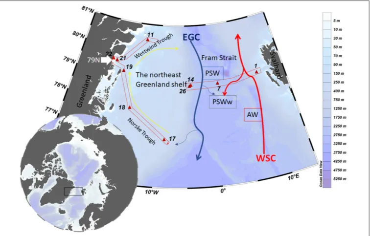
FIGURE 1 |Map of the study area and schematic currents in Fram Strait. The black square indicates the sampling location, and stations are indicated by red triangles. The West-Spitsbergen Current (WSC, red arrows) brings warm Atlantic Water (AW) into the Arctic Ocean. The southward flowing East Greenland (EGC, gray arrows) carries part of the recirculated WSC as well as outflow waters from the Arctic Ocean. The anti-cyclonic circulation through the Norske – Westwind Trough system is indicated by yellow arrows. These schematic currents are simplified fromSchaffer et al. (2017)and based onBourke et al. (1987). Figure was made using the software Ocean Data View (Schlitzer, 2018).

coupled plasma-mass spectrometry (HR-ICP-MS, Thermo Fisher Element XR) after pre-concentration (Rapp et al., 2017), the detailed procedure is described elsewhere (Krisch et al., 2020). Subsamples for a second DFe determination from the ligand bottles, was analyzed using HR-ICP-MS (Thermo Fisher Element XR) after pre-concentration using an automated SeaFAST system (SC-4 DX SeaFAST pico; ESI), and the quantification was done via standard additions. The procedure is described in detail inArdiningsih et al. (2020). DFe obtained from ligand samples was approximately 15% lower than DFe obtained from immediately acidified samples, as also found by others (Gerringa et al., 2016; Gerringa et al., 2019). DFe from ligand samples was used for the calculation of [Lt] and log K⁰_Fe⁰_L. The results of the determination in samples immediately acidified onboard and in subsamples taken from the ligand is attributed to either adsorption of Fe on the ligand bottle wall and possibly, even though we worked in laminar flow benches, contamination subsample from the ligand bottle, since this bottle was handled several times for the different applications.

In order to extrapolate DFe speciation to ambient DFe concentrations, DFe from the immediately acidified samples,

[Lt] and log K⁰_Fe⁰_L were used to calculate the excess ligand concentrations [L⁰] (i.e., concentration of ligands not bound to Fe). The [L⁰] was subsequently used to calculate the side reaction coefficient of the ligands (αFe⁰L), which is the product of logK⁰_Fe⁰_L and [L⁰]. The side reactions coefficient describes the effective affinity of a ligand for Fe, and takes into account the concentrations of the metal, the ligand and other competing cations thus describing the effective affinity between the natural ligands and Fe. The three different ALs used in the voltammetric methods (TAC, SA and NN) in this study will be indicated in subscript letters after the ligand parameters, e.g. [Lt]TAC or logK⁰_Fe⁰_L(TAC).

TAC Method

The analytical procedure of the here used TAC method is based onCroot and Johansson (2000), with modifications afterSlagter et al. (2017). The method is described in detail byArdiningsih et al. (2020) and uses a Hg drop electrode stand (VA663 Metrohm, Switzerland) connected to aµAutolab voltammeter and Nova 1.9 (Metrohm Autolab B.V., Netherlands) as the software user-interface. The titrations were done at pH 8.05 using 5 mM ammonium-borate buffer in the presence of 10µM

TAC and left to equilibrate for at least 8 h or overnight before voltammetric analysis. For each sample, duplicate scans were undertaken at a deposition time of 140 s, starting with the lowest added Fe(III) aliquot and working towards the highest added Fe(III) concentration. The Fe additions were 0; 0.2; 0.4;

0.6; 0.8; 1.0; 1.2; 1.5; 2.0; 2.5; 3.0; 4.0; 6.0; 8.0 nM, where the no Fe addition and the highest Fe addition vials were prepared in duplicate and both were analyzed. The limit of detection (LOD) was 0.016 nM eq. Fe, obtained as three times the noise in the scan.

SA Method

The SA method follows the protocol by Abualhaija and van den Berg (2014) with a low SA concentration (5 µM) and overnight (8 hours) equilibration, but using the BioAnalytical System (BASi) controlled growth mercury electrode coupled with an Epsilon ε2 (BASi) electrochemical analyzer (Buck et al., 2015). The voltammetry system was controlled by a computer using BASi Epsilon-EC as the interface software, and ECDsoft was used to quantify the peak height of the voltammetric scan.

Teflon vials (Fluorinated Ethylene Propylene (FEP), Savillex) were conditioned at least three times with seawater amended with buffer, DFe addition and SA. The first conditioning solution was changed immediately after rigorous shaking, followed by the next addition of conditioning solution, whereas the last conditioning solution was left at least for 8 h. The samples were buffered to a final pH of 8.2 with 5 mM of a boric acid- ammonium buffer. The titration consisted of 14 sub-sampled aliquots with Fe(III) standard additions of 0 to 3.0 nM with 0.5 nM intervals followed by concentrations of 4.0, 5.0, 6.0, 8.0, and 10 nM. The no addition and the highest addition were prepared in duplicate and both were analyzed. The chemical blank is measured in between samples to avoid carry over. For each sample, duplicate scans were done in a Teflon vial as voltammetric cell with a deposition time of 90 s. The LOD was 0.12 nM eq. Fe, obtained as three times the noise of our lowest standard (0.5 nM) in the scan.

NN Method

The analytical procedure for the NN method followed (Boye et al., 2001) and was adapted from the original NN method (Yokoi and van den Berg, 1992; Gledhill and van den Berg, 1994). Voltammetric analysis was performed using a mercury drop electrode stand model VA663 (Metrohm, Switzerland) connected to aµAutolab voltammeter (Metrohm Autolab B.V., the Netherlands).

Sample aliquots of 10 mL were buffered to pH 8.0 with 4- (2-Hydroxyethyl)piperazine-1-ethanesulfonic acid (HEPES; final concentration 0.01 M) and a final concentration of 2 µM NN was added. The addition of Fe (III) standards ranged from 0 to 10 nM with increments of 0.5 nM from 0 to 4.5 nM, followed by concentrations of 6.0; 8.0 and 10 nM. The sample mixtures were left to equilibrate overnight (≥12 h). The voltammetric scans were done in duplicate for each sample with a deposition time of 240 s. The LOD for the detection of FeNN₃, calculated using three times standard deviation of our lowest standard (0.5 nM)/slope

is 0.13 nM eq. Fe for samples analyzed using the conditions used in this study.

Calculation of Speciation Parameters

We define the side reaction coefficient describing the effective affinity of Fe binding to AL as D, in order to prevent confusion with the side reaction coefficient of the natural ligands. It is the product of logK⁰_Fe⁰_(AL)xand [AL], and calculated as (Table 1).

D = [AL]x K_Fe^{0 0}_(AL)xor D = [AL]^xxβ_Fe^{0 0}_(AL)x (1) The ‘upper’ limit of the detection window (Dw) is defined by the precision and detection limit of the analytical method (Laglera and Filella, 2015), whilst in an internally calibrated system, the lower limit is set by the assumption that all the weak ligand sites have been titrated within the range of added Fe concentrations, which can in practice be restricted by the linear range of the technique (Hudson et al., 2003).

For this study, we assumed that the width of the Dw is one order of magnitude above and below the center of detection window, D, as conventionally assumed in the literature (Apte et al., 1988; van den Berg et al., 1990; Hudson et al., 2003;

Pizeta et al., 2015).

The inorganic Fe side reaction coefficient (αFe⁰) is used to transform the conditional stability constant of AL with respect to Fe³⁺ into the one with respect to Fé (log K⁰ _Fe⁰_L).

As the buffer pH differed between the methods, the pH of analysis was slightly different for each AL, thus the value of αFe⁰ is different for each pH (Table 1). Ardiningsih et al.

(2020) used the value of αFe⁰ derived from Visual MINTEQ software (Gustafsson, 2011) with the ionic strength (I) is being calculated along with the determination of αFe⁰. In this study, the values of αFe⁰ were calculated based on the solubility products of the Fe-hydroxides at the fixed pH of analysis and I = 0.7 (Liu and Millero, 1999). As a result of different αFe⁰ values compared to previous results obtained with the TAC method, the resulted value of log K⁰_Fe⁰_L and log αFe⁰L

in this study are 0.1 higher than the results of TAC method reported byArdiningsih et al. (2020).

A non-linear model of the Langmuir isotherm (Gerringa et al., 2014) was used to interpret the ligand parameters, as described for the data obtained with the TAC method byArdiningsih et al.

(2020). A one- and two-ligand model was applied to the data, and the ligand parameters calculated were [L_t], logK⁰_Fe⁰_Land log αFe⁰L. In case of two ligand groups, the relatively strong ligand group was denoted with 1, the relative weak group with 2, as follows: [L₁]_TAC, and [L₂]_TAC, or logK⁰_1(TAC) and logK⁰_2(TAC). The sum of the concentration of [L₁] and [L₂] from the two- ligand model will be denoted as. The absolute difference between [Lt] values derived with two different method is referred to as δ[Lt] (i.e.δ[Lt]SA−TAC is the absolute difference between [Lt]SA

and [L_t]_TAC). Two ligand groups could not be resolved for the NN method. The mean sensitivity (S) obtained for the samples with the different methods were S = 3.97±0.70 (N = 70) for the TAC method, S = 76.4±23.0 (N = 69) for the SA method, and for the NN method S = 0.93±0.17 (N = 15).

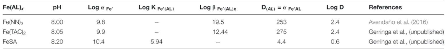
TABLE 1 |Summary of the formed Fe(AL)xcomplexes and the detection window of each voltammetric methods.

Fe(AL)x pH LogαFe⁰ Log KFe⁰(AL) LogβFe⁰(AL)x D_(AL)=αFe⁰AL Log D References

Fe(NN)3 8.00 9.8 − 19.5 253 2.4 Avendaño et al. (2016)

Fe(TAC)2 8.05 9.9 − 12.44 275 2.4 Gerringa et al., (unpublished)

FeSA 8.20 10.4 5.94 − 4.4 0.6 Gerringa et al., (unpublished)

RESULTS Hydrography

The water mass distribution and circulation are described elsewhere in detail (Rudels et al., 2005; Beszczynska-Möller et al., 2012; Rudels et al., 2015; Laukert et al., 2017; Richter et al., 2018). The selected stations in this study represent the main hydrographic features present in Fram Strait and on the northeast Greenland continental shelf (Figure 1; more details in Ardiningsih et al., 2020). Warm and saline (Temperature>2^◦C and Salinity > 35; Rudels et al., 2005; Laukert et al., 2017).

Atlantic Water (AW) is present at depths shallower than∼500 m in our stations. Cold and less saline (Temperature ≤ 0^◦C and Salinity < 34.5; Rudels et al., 2005) PSW is present on the western side (stations 14, 26) in the upper ∼300 m. AW recirculates in the upper 200 m in the central Fram Strait, forming warmer Polar Surface Water (PSWw) (Swift and Aagaard, 1981).

At about 500 to 900 m depth on both sides of Fram Strait, Atlantic Intermediate Water (AIW) (Rudels et al., 2005) exists above the Norwegian Sea Deep Water (NSDW) (Swift and Aagaard, 1981). In this study, AIW and NSWD are referred to as deep waters.

The Norske-Westwind Trough system is situated on the Northeast Greenland shelf (Figure 1). The surface water, PSW, follows this circulation flowing along the Norske Trough to the bay of the 79N Glacier and thereafter continues into the Westwind Trough. Deeper than 200 m, modified-AIW (mAIW) enters the Norske-Westwind Trough system, modified by physical mixing before being propagated toward the inner shelf (Topp and Johnson, 1997;Schaffer et al., 2017). The shallow sill in the Norske Trough restricts the flow of mAIW, causing the mAIW in the Norske Trough was 1^oC warmer than mAIW in the Westwind Trough (Schaffer et al., 2017), therefore in this study, it is referred to as warm-mAIW and cold-mAIW, respectively.

Fe Speciation Using a One-Ligand Model

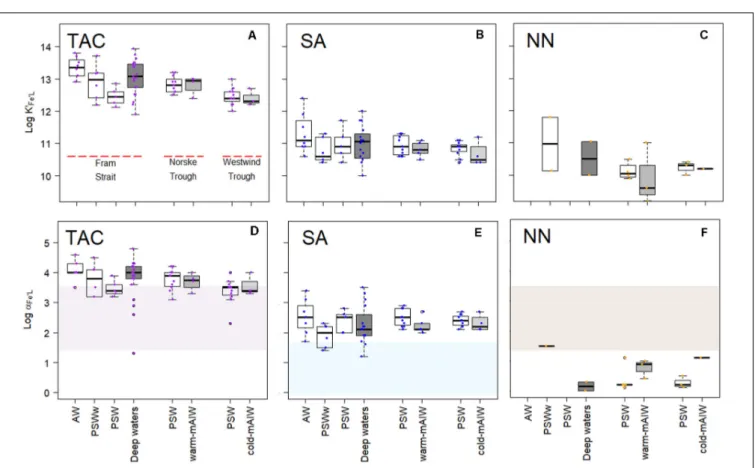
Total ligand concentration, [L_t], is calculated for each method and grouped based on the water masses existing in the different biogeochemical provinces (Figure 2). We observed similar trends for [L_t]_TAC, [L_t]_SAand [L_t]_NNin various waters (Figures 2A–C;

the number of samples for each water masses is given inTable 2), with an increase in the median [L_t] from Fram Strait to the Norske Trough and highest values at the glacier front and in Westwind Trough. The absolute values of [Lt] derived via the three different methods differed considerably. The [L_t]_SA (median = 2.82 nM eq. Fe) was highest followed by [L_t]_TAC (median = 1.79 nM eq. Fe) and [L_t]_NN(median = 0.96 nM eq.

Fe). In Fram Strait, the ratio of [L_t]_TAC /[L_t]_SAvaried between 0.6 to 1, however, on the shelf, this ratio was nearly constant

at approximately 0.6 (median,Figure 3A). The ratio of [L_t]_NN /[L_t]_SA was 0.2 – 0.5 in Fram Strait and 0.2 – 0.8 over the shelf (Figure 3B).

For individual voltammetric methods, the variation in log K⁰_Fe⁰_L values reached up to two orders of magnitude between samples (Figures 4A–C). The variation in logK⁰_Fe⁰_L values in Fram Strait was larger than on the shelf. The most constant but lowest log values were observed in Westwind Trough. The value of logK⁰_Fe⁰_Lwas highest for TAC, logK⁰_Fe⁰_L(TAC)(median = 12.8), followed by log K⁰_Fe⁰_L(SA) (median = 10.9) and log K⁰_Fe⁰_L(NN) (median = 10.1; Supplementary Figure 1a). The differences in logK⁰_Fe⁰_Lvalues between the methods are significant (p<0.05;

Supplementary Figure 1a). For NN, median logK⁰_Fe⁰_L(NN)values were significantly lower and ranged from 9.8 to 11.0 (Figure 4C andTable 2). For the determination of logK⁰_Fe⁰_L,the curved part is essential. In the non-linear transformation of the Langmuir isotherm, log K⁰_Fe⁰_L is derived by dividing the tangent of the curve at the lowest determined Fe concentration by the total ligand concentration. However, because ligand concentrations are typically ca. 1 nM eq. Fe in excess of the dissolved Fe concentration, an inability to detect the first titration point and a lower number of points in the curved part of the titration will mean that the tangent of the curve at the first detectable Fe concentration will be considerably lower than the tangent that would have been observed at the ambient DFe concentration and this will lead to an underestimation in logK⁰_Fe⁰_L(e.g., for a samples with 0.5 nM DFe and a ligand concentration of 1.5 nM eq. Fe, 66 % of the ligands are titrated already at the first titration point of DFe+0.5 nM added). Thus, this difference likely arises because the peak with 0 Fe addition was usually not detected, which compromises the estimate of logK⁰_Fe⁰_L(NN). Furthermore, for some samples the titration curves were nearly linear and the difference between the determined FeNN₃concentration and the expected Fe concentration was too low to detect so that values of logK⁰_Fe⁰_L(NN)and logαFe⁰L(NN)could not be estimated.

A relatively wide range in logα Fe⁰L for both TAC and SA methods was observed in Fram Strait, whereas on the shelf, logαFe⁰Ldecreased with depth. The median logαFe⁰L(TAC)(3.8) was highest compared to log αFe⁰L(SA) (2.3) and log αFe⁰L(NN)

(0.6) (Supplementary Figure 1b). The values of logαFe⁰L(TAC)

and log αFe⁰L(SA) fell within and on the upper limit of log Dw (Figures 4D,E), whereas the values of logαFe⁰L(NN) mostly fell below the lower limit of log Dw (Figure 4F).

Fe Speciation Using a Two-Ligand Model

For both the TAC and SA methods, two ligand groups could be resolved in some of the samples, mostly the shelf samples (Figures 5A,B). Only 10% (4 out of 39) of samples from the Fram Strait could be resolved for two ligands using the TAC

FIGURE 2 |Box plot of ligand concentrations, [Lt], in nM eq. Fe from three different applications of added ligands(A)TAC,(B)SA, and(C)NN, as fitted (non-linear) by a one-ligand model using the Langmuir isotherm. The data is grouped by the biogeochemical provinces as described byArdiningsih et al. (2020). A thick horizontal line indicates the median, the box contains the first to third quartiles, the whiskers are the range of data excluding the outliers and the circles indicate the outliers being 1.5* interquartile range from the box (Teetor, 2011). Figures were made using the software package R.

TABLE 2 |Summary of the mean and median total ligand concentrations [Lt], conditional stability constants logK⁰Fe⁰L, and the side reaction coefficients log , from the three applications of added ligands (TAC, SA and NN) according to the one-ligand model.

one-ligand model Water masses [Lt] Log KFe⁰L LogαFe⁰L

TAC SA NN TAC SA NN TAC SA NN

Fram Strait AW Mean (n) 1.17(6) 2.06(8) NA 13.3 11.4 NA 4.1 2.6 NA

Median 1.20 1.99 NA 13.2 11.2 NA 4.0 2.5 NA

PSWw Mean (n) 1.84(6) 1.91(6) 0.75(2) 12.9 10.8 11.0 3.8 1.9 1.2

median 1.77 1.70 0.75 13.0 10.6 11.0 3.8 2.0 1.2

PSW Mean (n) 1.65(5) 2.63(5) NA 12.5 11.0 NA 3.5 2.4 NA

Median 1.78 1.94 NA 12.4 10.9 NA 3.4 2.5 NA

deep waters Mean (n) 1.58(21) 2.19(16) 0.72(3) 13.0 11.0 10.5 3.6 2.2 1.2

Median 1.35 2.01 0.62 13.0 11.1 10.5 3.9 2.1 1.2

Norske Trough PSW Mean (n) 2.03(11) 3.38(11) 0.90(6) 12.8 10.9 10.1 3.8 2.5 0.6

median 1.96 3.55 0.75 12.8 10.9 10.1 3.9 2.5 0.5

mAIW warm Mean (n) 1.65(4) 2.51(5) 1.26(6) 12.8 10.9 10.2 3.7 2.3 1.0

Median 1.68 2.21 1.25 12.9 10.8 9.8 3.7 2.1 0.7

Westwind Trough PSW Mean (n) 2.19(11) 3.61(11) 1.37(3) 12.4 10.8 10.2 3.4 2.4 0.8

Median 2.17 3.76 1.05 12.4 10.9 10.3 3.5 2.4 0.5

mAIW warm Mean (n) 2.21(4) 3.71(4) 2.31(1) 12.4 10.7 10.2 3.5 2.3 1.4

Median 2.20 3.85 2.31 12.3 10.5 10.2 3.4 2.2 1.4

The data are grouped based on water masses present in the different biogeochemical provinces as described byArdiningsih et al. (2020). The bold values are the amount of samples for each category.

and SA methods, therefore, it is not possible to make a statistical comparison of the results of TAC and SA in the Fram Strait using the two-ligand model. On the shelf two ligands could be resolved for about 26% (8 out of 30) of the samples using TAC and 77%

(24 out of 31) of the samples using the SA method.

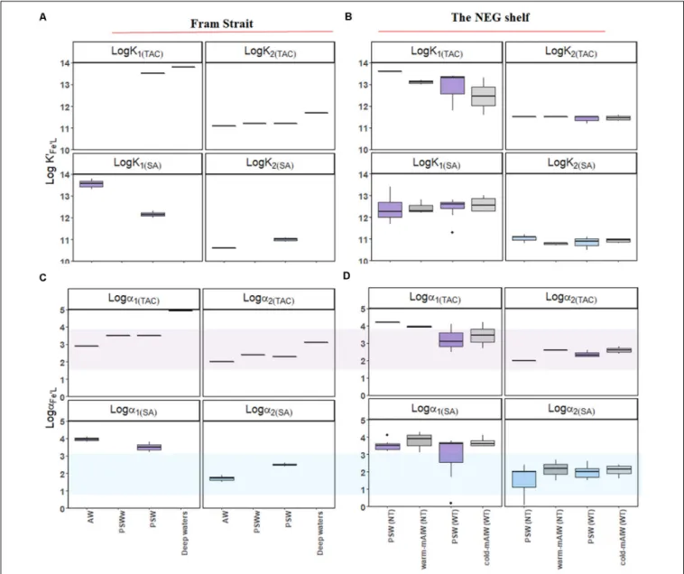
Using the TAC method, [L₁]_TAC, ranged from 0.48 to 2.66 nM eq. Fe (Figures 5A,B) with values of logK⁰_1(TAC) between 11.6 and 14 (Figures 6A,B). In comparison, [L₂]_TACvaried between 0.30 to 3.10 nM eq. Fe with logK⁰_2(TAC)between 11.1 and 11.7.

The values of logα2(TAC)and logα1(TAC)were mostly within log Dw for TAC, with an exceptions some logα1(TAC) values were higher than the upper limit of log Dw (Figures 6C,D).

Using the SA method, [L₁]_SA ranged from 0.82 to 3.87 nM eq. Fe and [L₂]_SA from 0.08 to 3.43 nM eq. Fe. The values of logK⁰_1(SA)ranged from 11.3 to 13.8 and logK⁰_2(SA)from 10.5 to 11.2. Similar values of logα1(SA)were higher than log Dw, and logα2(SA)values fell within log Dw (Figure 5B).

DISCUSSION

In the below discussion the ligand parameters (log K⁰_Fe⁰_L, log αFe⁰Land [L_t]) derived from each method are related to Dw of the three ALs. Using different Dw, the ‘target ligand pool’ shifts,

FIGURE 3 |Boxplot showing the difference in ligand concentrations obtained by TAC, SA and NN, [Lt]TAC, [Lt]SAand [Lt]_NN,respectively.(A)the absolute difference in concentrations [Lt]TAC- [Lt]SA(nM eq. Fe), the relative ratio of(B)[Lt]TAC/ [Lt]SAand(C)[Lt]NN/ [Lt]SA. The details of the boxplot are described inFigure 2caption.

FIGURE 4 |Boxplot of the conditional stability constants (logK⁰Fe⁰L,A–C) and side reaction coefficients (logαFe⁰L,d,e,f) from three different methods using TAC, SA and NN as the AL. The shades in(D–F)indicate the detection window (log Dw) for each method. The details of the boxplot are described inFigure 2.

and it is thus appealing to use the different Dw to distinguish different fractions of binding sites. However, the precision of the Dw, its value and thus the conditional stability constant of AL (K⁰_Fe⁰_AL orβFe⁰AL) with Fe must be considered. In order to properly evaluateK⁰_Fe⁰_AL orβFe⁰AL, we must therefore consider uncertainties in the determination of K⁰_Fe⁰_AL or βFe⁰AL. For example, ionic strength, the side reaction coefficients of the calibration ligand and the pH of the analysis could lead to subtle

but important differences in Dw (Gledhill et al., 2015;Laglera and Filella, 2015;Ye et al., 2020).

The calibration of the competing AL is done by comparing the well-defined logαvalue of calibrating ligand, such as EDTA and diethylenetriaminepentaacetic acid (DTPA) with D. The corrections for ionic strength, the choice of the calibrating ligand side reactions and differences in pH have consequences for the resultingK⁰_Fe⁰_AL and/orβFe⁰AL. Errors obtained during the

FIGURE 5 |Boxplot of the results from a two-ligand model: ligand concentrations of the strong ligand group [L1], and the relatively weak ligand group [L2], together with the sum of [L1] and [L2] from samples(A)from Fram Strait and(B)from the northeast Greenland shelf. The details of the boxplot are described inFigure 2.

derivation of D for the methods applied here range from<log 0.1 to log 0.9 (Gledhill and van den Berg, 1994;Rue and Bruland, 1995;Croot and Johansson, 2000;Abualhaija and van den Berg, 2014). From unpublished results of repeated calibrations, we have also found standard deviations inK⁰_Fe⁰_ALand/orβFe⁰ALbetween log 0.5 and log 1 for D.

In addition, uncertainties can emanate during the interpretation of titration data. The competition between AL and the natural ligands determines log K⁰_Fe⁰_L obtained where Fe additions filled the natural ligand sites, forming the curved part of the titration. The number of data points in the curved part hardly affects the calculation of [L_t], but a lack of data points here propagates high standard deviation in the estimation of log K⁰_Fe⁰_L. This causes a high standard deviation in log K⁰_Fe⁰_L in relatively saturated natural organic ligands. In the linear part of the titration, the number of data points affects both the values of [L_t] and log K⁰_Fe⁰_L (Gerringa et al., 2014).

Therefore, in our data we expect larger errors inK⁰_Fe⁰_Lestimated by SA and NN because these methods had fewer data points in the range of 0-1.5 nM added Fe (steps of 0.5 versus 0.2 nM Fe added). Indeed, larger error in estimation of log K⁰_Fe⁰_L(SA) and log K⁰_Fe⁰_L(NN) relative to log K⁰_Fe⁰_L(TAC) were observed¹. Moreover, the sensitivity, which transforms the peak current (nA) into Fe concentration (nM), is obtained also from the slope of the linear part of the titration (Hudson et al., 2003).

At high [Lt] it is possible that the linear part is not reached yet, and the titration curve is not truly linear, introducing an error in the estimation of S and [L_t]. The nonlinear Langmuir approach should compensate for this source of error in the

1https://doi.org/10.25850/nioz/7b.b.7

data (Turoczy and Sherwood, 1997; Hudson et al., 2003;

Gerringa et al., 2014).

The quality of the titration curves is given by the standard deviation of [L_t] and logK⁰_Fe⁰_L.The variation of duplicate scans, especially in the first few points and at the high end of the titration could have large impact on the quality of the titration curves, adding uncertainties in the [L_t] and logK⁰_Fe⁰_L, respectively. The zero Fe addition was done and measured twice to ensure that the measurement was not influenced by unconditioned cell. The variation of duplicate scans at low Fe addition could go up to 50%. The zero Fe addition was different from the blank only in a few samples containing near saturated ligands. The variation of duplicate scans at the high end of the titration affects the linear part of the titration curve, and thus the determination of [L_t], log K⁰_Fe⁰_L and S. Therefore, the highest point Fe addition was done twice and measured with duplicate scans. At the highest Fe addition, the difference between duplicate scans was sometimes quite large, i.e. outliers were more than 20% different from the linear stretch (between 2 and 6 nM additions).

Other sources of uncertainty might come from the nature of the ligands. The heterogeneity of binding sites of large humic type molecules induces uncertainty depending on the saturation of the natural ligands with Fe. In this case, DFe concentration influences the outcome of the titration together with the detection window (Gledhill and Gerringa, 2017). Overall, the following discussion is limited to the above-mentioned uncertainties and the assumptions used on the calculations.

One-Ligand Model

The different detection windows reflect the ability of the methods to detect ligands (Gledhill and Gerringa, 2017) that are

FIGURE 6 |Boxplot of the results from a two-ligand model: the conditional stability constants of the relatively strong (logK⁰1) and weak ligand groups (logK⁰2) from samples(A)from Fram Strait and(B)from the northeast Greenland shelf; side reaction coefficients of the relatively strong (logα1) and weak ligand groups (logα2) from samples(C)from Fram Strait and(D)from the northeast Greenland shelf. The application of TAC and SA are indicated in subscribed letters. The shades in(C) and(D)indicate the detection window (log Dw) for each method. The details of the boxplot are described inFigure 2.

characterized by a range of logαFe⁰L. The detection windows of the SA, NN and TAC methods overlap (log Dw_(SA)= 0 – 1.6;

log Dw_(NN) and log Dw_(TAC) = 1.4 – 3. 4). Nevertheless, the resulting median values for logαFe⁰L from the natural samples differ one order of magnitude between methods (SA: 1.2 – 3.5;

TAC: 1.3 – 4.8; NN: 0.2 - 1.9; Table 2). Having the lowest Dw, the SA method detected ligands with log αFe⁰L values in between the other two methods (Figure 4E), and always had the highest [L_t] (Figure 2B), whereas log K⁰_Fe⁰_L obtained from each method varied for SA: logK⁰_Fe⁰_L10 – 12.4, NN: logK⁰_Fe⁰_L 9.2 – 11.8 and TAC: logK⁰_Fe⁰_L 11.9 - 13.9¹. The three methods thus appear to detect different ligand pools in the same samples.

However, considering an error of±0.5 - 1 due to uncertainties in

calibration of the AL, NN and SA could have detected the same ligand group, albeit with different concentrations. With TAC we might have detected a different and stronger ligand group, compared to the results of the other two methods.

Many of the logαFe⁰Lvalues were above the upper limit of Dw for data using the TAC and SA methods (Figures 4D,E), which agrees with reported data using the same analytical procedures (Buck et al., 2015; Gerringa et al., 2015). Buck et al. (2015) reported a range of logαFe⁰Lfrom 2.5 to 3.5 (in theirFigure 4C) with log D = 1.8, whereasGerringa et al. (2015)reported logαFe⁰L

values that varied from∼3.0 to 4.0 (in theirFigure 4) with log D = 2.4. Observations of logαFe⁰L above log Dw are relatively common (Caprara et al., 2016), which can be explained by the

titration process. During a titration with Fe, [L⁰] decreases as the binding sites get filled with Fe, and consequently decreases the capacity of natural ligands to bind Fe (αFe⁰L= [L’]^∗K⁰_Fe⁰_L), whereas the capacity of AL (αFe⁰AL) is assumed to be constant (Gledhill and Gerringa, 2017). The equivalence point of the titration is the point at whichαFe⁰L= D. If during the titration, the αFe⁰L crosses Dw, then values of αFe⁰L can be estimated.

However, if the curve is not evenly weighted (i.e., more titration points lie below D_w than above as is usually the case), then the estimate may be biased. Furthermore, ifαFe⁰L is below Dw, then the data must be treated with care, since the values of log αFe⁰L became even lower with the Fe additions during the estimation. This is the case for almost all results obtained with NN and possibly arises as result of the lower sensitivity of the NN method, since this impacts both on the detection limit and the precision of the method. In practice this means that Dw for NN is likely to be narrower than that for SA and TAC and that NN could underestimate logK⁰_FeL(NN)using the CLE-AdCSV metal titration approach.

The median value ofδ[Lt]SA−TAC in PSW in western Fram Strait was 0.9 nM eq. Fe, whereasδ[Lt]SA−TAC in PSW on the shelf increased to 1.5 nM eq. Fe and 1.7 nM eq. Fe, respectively, in the Norske Trough and in the Westwind Trough (Figure 3C).

According toLaglera et al. (2011), the TAC method cannot detect part of the HS, and the NN method not sufficiently sensitive enough to elucidate stronger HS binding sites at nanomolar Fe concentrations in seawater. No consensus exists, however, on the underestimation of the HS ligands by the TAC method (Gerringa et al., 2007;Batchelli et al., 2010;Slagter et al., 2017;Dulaquais et al., 2018).Slagter et al. (2019)concluded that the TAC method can detect HS ligands when these ligands are either present at high concentrations or of a specific chemical composition. This could explain the lower [L_t] obtained with the TAC and NN methods compared to the SA method, and may even support the above reasoning using D. Since HS are heterogenous - with a distribution of ligand sites- HS does not therefore itself fit into

‘one group’ of ligands as determined by CLE-CSV. Moreover, the observable heterogeneity of ligand binding sites in samples is reduced at a higher detection window, thus a group of binding sites can be missed by an AL with a higher detection window (Gledhill and Gerringa, 2017). As such, the presence of HS as part of the ligand pool, can to some extent explain the difference in results between the methods. The PSW-flow via the TPD from the Arctic likely transfers HS ligands (Laglera et al., 2019a;Slagter et al., 2019). Approximately 62% of the Fe-binding ligands are humics in the TPD flow path in the Arctic (Sukekava et al., 2018), and thus [Lt]TAC is probably underestimated for the NN method, the influence of HS on the results obtained were only for measurements at high NN concentrations when HS possibly cannot compete with NN (Laglera et al., 2011). However, NN ([NN] = 5 µM; log D = 2.9) has successfully been used to assess DFe speciation in Antarctic sea ice (Lannuzel et al., 2015;

Genovese et al., 2018).

The [Lt]TACand [Lt]SAcapture the same trend of increasing concentrations from Fram Strait to Norske Trough and Westwind Trough (Figures 2A,BandSupplementary Figure 2a) with a fairly constant ratio of [L_t]_TACover [L_t]_SAin PSW (median

[L_t]_TAC/[L_t]_SA = 0.6; Figure 3B). The absolute differences, δ[L_t]_SA−TAC, varied in Fram Strait, where the HS influence possibly also varied, because the PSW-flow in western Fram Strait likely contains Arctic HS ligands. This suggests that HS play a role in the different results by the TAC and SA methods, however, the constant ratio ∼0.6 suggests a systematic offset between two methods, similar to the earlier studies (Buck et al., 2016;Slagter et al., 2019).Buck et al. (2016)concluded that TAC measurements fromGerringa et al. (2015) determined roughly half the ligand concentrations measured by the 25 µM SA method (Buck et al., 2012) at the BATS station in the Western Atlantic near Bermuda. Comparing the TAC and 25 µM SA methods,Slagter et al. (2019)found a ratio of 0.6 in the Arctic Ocean as well, remarkably both in and outside the influence of the HS-rich TPD. It must be noted that the 25µM SA method is different in concentration and equilibration time from the SA method used in our study, indicating the offset likely appears irrespective to the used analytical procedure. In addition, even though a ratio near 0.6 is often found, the offset is irregular in Fram Strait outside PSW as we find ratios varying between 0.6 and 1 (Figure 3B). Thus, the question remains, does the TAC method underestimate the ligand concentration because it cannot detect part of the ligands or does SA method overestimate the ligand concentration?

An offset caused by HS should result in varying ratios of [L_t]_TAC/[L_t]_SA with a varying relative amount of HS, as shown in the value of δ[L_t]_SA−TAC. However, no relationship between HS and [L_t]_TAC/[L_t]_SAwas observed in a previous study (Slagter et al., 2019) and we also did not see difference between the ratio of [Lt]TAC/[Lt]SA in HS-rich PSW compared to HS-poor AW (Figure 3B). Therefore, the difference between TAC and SA cannot solely be ascribed to their respective abilities to detect ligand groups in HS.

To conclude, the method with the highest detection window, i.e., TAC can detect a strong ligand group, and possibly misses weaker ligand groups, which were detected by the method with a lower detection window, SA. In contrast, despite having D_w similar to TAC, The use of NN results in both a lower [L] and log K⁰_Fe⁰_L. The application of multiple methods as suggested byBuck et al. (2012)thus requires careful consideration. Nevertheless, our results showed that the one ligand model captured a similar trend in [Lt] for all three AL, and [L] increased from Fram Strait to the Norske Trough to the Westwind Trough (Figure 2).

Two-Ligand Model

A one and a two-ligand model were fitted in the same dataset. The one-ligand model gives an overall bulk result of what is present to facilitate the comparison of all samples. The two-ligand model worked only in a few samples where two ligand groups were different enough to be distinguished. Even though the two-ligand model did not work in some samples, this does not mean that the diversity is less, only that the diversity obscures that two groups can be detected.

A strong and progressively weaker ligand group was distinguished (Figures 6A,B) by the methods using TAC and SA as AL. Distinguishing two ligand groups is possible when ligands are distinct enough, although this depends on data