aAtmospheric and Oceanic Sciences Program, Princeton University, Princeton, New Jersey
bDepartment of Atmospheric and Oceanic Sciences, McGill University, Montreal, Quebec, Canada
cResearch School for Earth Sciences, Australian National University, Canberra, Australian Capital Territory, Australia
dNOAA/Geophysical Fluid Dynamics Laboratory, Princeton, New Jersey
eGEOMAR Helmholtz Centre for Ocean Research Kiel, Kiel, Germany
fJoint Institute for the Study of the Atmosphere and Ocean, University of Washington, Seattle, Washington
(Manuscript received 9 August 2016, in final form 16 June 2017) ABSTRACT
The Weddell Sea polynya is a large opening in the open-ocean sea ice cover associated with intense deep convection in the ocean. A necessary condition to form and maintain a polynya is the presence of a strong subsurface heat reservoir. This study investigates the processes that control the stratification and hence the buildup of the subsurface heat reservoir in the Weddell Sea. To do so, a climate model run for 200 years under preindustrial forcing with two eddying resolutions in the ocean (0.258CM2.5 and 0.108CM2.6) is investigated.
Over the course of the simulation, CM2.6 develops two polynyas in the Weddell Sea, while CM2.5 exhibits quasi-continuous deep convection but no polynyas, exemplifying that deep convection is not a sufficient con- dition for a polynya to occur. CM2.5 features a weaker subsurface heat reservoir than CM2.6 owing to weak stratification associated with episodes of gravitational instability and enhanced vertical mixing of heat, resulting in an erosion of the reservoir. In contrast, in CM2.6, the water column is more stably stratified, allowing the subsurface heat reservoir to build up. The enhanced stratification in CM2.6 arises from its refined horizontal grid spacing and resolution of topography, which allows, in particular, a better representation of the restratifying effect by transient mesoscale eddies and of the overflows of dense waters along the continental slope.
1. Introduction
The Weddell Sea polynya refers to the immense sea ice–free area that occurred in the open-ocean region of the Weddell Sea in the winters of 1974–76 (Carsey 1980).
Because it opens a window between the atmosphere and deep ocean through intense deep convection, the Wed- dell Sea polynya is thought to have a substantial impact on the climate [seeMorales Maqueda et al. (2004)for a review], including on the regional atmospheric circula- tion (e.g., Moore et al. 2002), the global overturning circulation (e.g., Martin et al. 2013, 2015), deep and bottom water properties (e.g.,Zanowski et al. 2015), and
oceanic carbon uptake (Bernardello et al. 2014). That the Weddell Sea polynya was only observed once (Carsey 1980) makes it a feature difficult to fully un- derstand on an observational basis. On the other hand, many ocean models simulate the Weddell Sea polynya as a recurring feature (Heuzéet al. 2013;Martin et al.
2013). Modeling studies have shown that the represen- tation of stratification is key to the occurrence of the polynya. Increased stratification, as a result of strong freshwater fluxes at the surface, was found to hamper the formation of the polynya (de Lavergne et al. 2014;
Stössel et al. 2015; Kjellsson et al. 2015). In contrast, decreased stratification, resulting from weak vertical mixing and the subsequent buildup of a high salinity bias at the surface, was found to favor the occurrence of the polynya (Kjellsson et al. 2015;Heuzéet al. 2015).
The Weddell Sea polynya forms following a de- stabilization of the stratification leading to vertical mixing of warm deep waters to the surface that initially slows down the growth of sea ice and eventually prevents
Corresponding author: Carolina Dufour, carolina.dufour@
mcgill.ca
Denotes content that is immediately available upon publica- tion as open access.
DOI: 10.1175/JCLI-D-16-0586.1
Ó2017 American Meteorological Society. For information regarding reuse of this content and general copyright information, consult theAMS Copyright Policy(www.ametsoc.org/PUBSReuseLicenses).
its formation (e.g., Martinson et al. 1981; Goosse and Fichefet 2001). The heat brought to the surface originates from a reservoir of relatively warm waters [;(0.58–18C)]
in the subsurface [;(300–1500 m)];Gordon 1998). Once the polynya is formed, the surface ocean is directly ex- posed to the freezing atmosphere (;2308C) inducing a strong cooling of surface waters that eventually become dense enough to sink to the deep ocean. The sinking waters are replaced by the more buoyant subsurface waters that are cooled down and the vertical exchange continues. An intense chimney of deep convection (;3000 m;Gordon 1978) thus takes place in the polynya region. The polynya closes once the convection shuts down owing to the depletion of the subsurface heat res- ervoir (Martinson et al. 1981;Martin et al. 2013) or an excessive input of freshwater at the surface (Comiso and Gordon 1987). Hence, the buildup of a heat reservoir in the subsurface is a necessary precondition for the occur- rence and maintenance of the polynya.
Aside from the polynya events, the heat reservoir is maintained in the subsurface by a salinity-controlled stratification. In winter, a thin layer (;100 m) of rela- tively fresh and near-freezing waters caps the heat reser- voir (;34.4 psu;21.88C;Gordon 1998). The heat reservoir is established by the inflow of the warm and saline Lower Circumpolar Deep Waters (LCDW;.34.67 psu;.0.28C;
Seabrooke et al. 1971), which enter the Weddell Sea through the large-scale cyclonic gyre (Fahrbach et al.
1994). Below the heat reservoir, relatively fresh and cold waters (34.60 , salinity , 34.67 psu; ;20.48C;
Seabrooke et al. 1971) are found again. These waters comprise the Antarctic Bottom Waters (AABW) that originate from waters formed on the continental shelves (Orsi et al. 1999), which are dense enough to spill over the continental slope (e.g., Morales Maqueda et al. 2004).
The stratification of the Weddell Sea is characterized by a large-scale doming of isopycnals near the center of the Weddell Gyre, which brings the subsurface heat reservoir close to the surface and a downward sloping of isopycnals toward the continental slopes (Gordon et al. 1981). This large-scale spatial structure of isopycnals is mainly driven by the wind stress curl (Gordon et al. 1981). The char- acteristics of the subsurface heat reservoir are thus closely tied to the gyre circulation and the vertical stratification in the Weddell Sea.
The impact of the stratification on the occurrence of the Weddell Sea polynya has been investigated by sev- eral recent studies (e.g.,de Lavergne et al. 2014;Stössel et al. 2015; Kjellsson et al. 2015). These studies have demonstrated the role played by the surface forcing, in particular freshwater fluxes, on the destabilization of the stratification and subsequent triggering of the Weddell Sea polynya. In this study, we investigate which
processes help maintain the stratification in the Weddell Sea, hence allowing for the buildup of the subsurface heat reservoir. Investigating the triggering of the po- lynya is beyond the scope of our study. To do so, we compare a 0.108climate model to its 0.258counterpart and find that, in contrast to the 0.108model, the 0.258 model resolves a weaker vertical stratification in the Weddell Sea leading to the buildup of a weaker sub- surface heat reservoir. In addition, the weaker stratifi- cation makes the 0.258 model prone to simulate quasi-continuous deep convection events, in contrast to its higher-resolution counterpart, which simulates two large polynyas over the 200-yr simulation, separated by periods of relatively strong stratification. We find that the weak stratification of the 0.258model arises in par- ticular from a poor representation of the ocean meso- scale and dense water overflows, as well as from the deep convection events themselves. This paper thus demon- strates that better resolving ocean mesoscale processes and overflows has an important impact on the stratifi- cation of the Weddell Sea, and as such on the pre- conditioning of the Weddell Sea polynya.
2. Methods
a. Models and simulations
1) MODELS
We use CM2.5 and CM2.6, two models of the GFDL CM2-O climate model suite first introduced by Delworth et al. (2012)and further analyzed byGriffies et al. (2015). Both models use the same atmosphere of roughly 50-km resolution and identical sea ice and land models. The two models only differ by the horizontal resolution of the ocean component. CM2.5 has a nomi- nal ocean grid spacing of 0.258and CM2.6 of 0.108, which correspond to a grid size of 9.5 and 3.8 km, respectively, at 708S. Neither of these models fully resolves mesoscale eddies in the high latitudes of the Weddell Sea. The resolution of the first baroclinic Rossby radius of de- formation on the continental shelves requires a grid spacing on the order of 1 km (Hallberg 2013; Stewart and Thompson 2015), which corresponds to a nominal grid spacing on the order of1/388, thus remaining out of reach of the current climate models. Both models nonetheless produce energetic ocean currents in the Weddell Sea, with a gyre circulation mostly carried by the Antarctic Slope Current (ASC;Fig. 1). The ASC is stronger in CM2.6 than in CM2.5, in particular where it flows to the southwest along the Queen Maud Land (;208W) and to the north along the shelf of the Ant- arctic Peninsula (;558W). On the continental shelves,
mean along-coast currents are simulated with a similar magnitude in the two models. However, these currents show more spatial structure with finer jets in CM2.6 than in CM2.5. In CM2.6, as troughs and other bathymetric depressions are better resolved, the flow gets steered by a more complex topography.
The oceanic component of CM2.5 and CM2.6 is based on the Modular Ocean Model, version 5 (MOM5;
Griffies 2012), run with volume-conserving Boussinesq kinematics and a z* vertical coordinate. The vertical grid has 50 levels with a thickness of 10 m at the surface increasing with depth to 210 m. Both models use the K-profile parameterization (KPP) boundary layer scheme, which includes a downgradient vertical diffusion term and a nonlocal transport term (Large et al. 1994). Mixing schemes for gravitational instability, shear instability, and double diffusion (Large et al. 1994) are also used, as well as mixing schemes for internal tides (Simmons et al.
2004) and coastal tides (Lee et al. 2006). There is no static background diffusion in the models. In addition, no pa- rameterization of overflows or representation of ice-shelf cavities is used. No mesoscale eddy transport parame- terization is used in the tracer equation in either model,
so that a clear comparison of the effect of resolved me- soscale processes on the two model solutions can be made. To account for the restratification effect from submesoscale eddies in the mixed layer, the parameter- ization of Fox-Kemper et al. (2011) is used in both models. Finally, both CM2.5 and CM2.6 are coupled to a biogeochemical model called miniBLING [seeGalbraith et al. (2015)for a description of the model]. In our ana- lyses, dissolved oxygen (O2) from miniBLING is used as a tracer of ocean ventilation.
The use of fully coupled climate models run with eddy-modest to eddy-active ocean resolutions, and set up in the same configuration with minimal use of pa- rameterizations, offers a rigorous framework to assess the effects of ocean mesoscale processes and refined topography in the buildup of the subsurface heat reser- voir in the Weddell Sea.
2) SIMULATIONS
CM2.5 and CM2.6 are each run for 200 yr under 1860
‘‘preindustrial’’ atmospheric radiation based on a con- stant globally averaged CO2mixing ratio of 286 ppm by volume (ppmv). The ocean is started from rest with
FIG. 1. Depth-averaged current speed [log10(m s21); color shading] and annual sea ice extent (solid thick black line) averaged over years 106 to 125 in (left) CM2.5 and (right) CM2.6. The thin solid black line indicates the 1000-m isobath. The green box displays the region of our study, referred to as the Weddell Sea region. (right) The dashed thick black line shows the winter (September) sea ice extent for year 128 of CM2.6. The closed black-dashed contour on the northeast side of the Weddell Sea region corresponds to the first polynya that occurs in CM2.6. This polynya opens in year 126 at Maud Rise (seeFig. 2) and grows over the first 3 yr until year 128 when it reaches a shape that resembles the observed polynya of the 1970s (Carsey 1980). In year 128, the size of the modeled polynya is 113105km2(based on a sea ice concentration,75%). For comparison, the Weddell Sea polynya observed in the 1970s was around 2–33105km2(Carsey 1980). From year 129, the polynya continues growing and drifting westward while becoming an embayment rather than a hole.
temperature and salinity fields initialized toWorld Ocean Atlas 2009(WOA09;Antonov et al. 2010;Locarnini et al.
2010). A brief evaluation of the Southern Ocean state of the last 20 years of the CM2.6 preindustrial simulation can be found inDufour et al. (2015). For a global eval- uation of the two models, the reader is referred toGriffies et al. (2015), where 1990 radiatively forced simulations with CM2.5 and CM2.6 are compared.
b. Domain and period of analysis
Our study focuses on the region that extends in lon- gitude from the west of Maud Rise to the Antarctic
Peninsula (108–638W), and in latitude from the tip of the Antarctic Peninsula to the Antarctic continent (south of 638S;Fig. 1). In the following, we refer to this region as the Weddell Sea region.Figure 1shows that the Weddell Sea region encloses well the polynyas that develop in CM2.6, which is where the polynya of the 1970s was observed. In the model, polynyas start at Maud Rise and widen as they drift westward with the Weddell Gyre flow (Fig. 2), in agreement with obser- vations (Carsey 1980). Maud Rise is known as a pref- erential site for deep convection, and many small polynyas have been observed there since the 1970s
FIG. 2. (top) Topography (gray shades) of the South Atlantic sector of the Southern Ocean in CM2.6 with the green box indicating the region where the Hovmöller diagram in the bottom panels is computed. (bottom) Hovmöller diagram (time vs longitude) of annual mean age tracer averaged between 658and 708S and over the whole water column for (left) CM2.5 and (right) CM2.6. The age tracer is normalized by the maximum age in the region every year, so that blue corresponds to the youngest waters and red to the eldest waters for each year. The horizontal dashed lines indicate the two time periods analyzed, respectively, years 106 to 125 and years 181 to 184 (seesection 2b). The Weddell Gyre contains relatively old water while the continental shelves are where new water forms. In CM2.6, the two large blue regions that extend between Maud Rise and the continental shelves correspond to two open-ocean polynyas that start around years 126 and 185, respectively, and last for around 20 yr. The two polynyas are initiated around Maud Rise and widen while being advected westward by the Weddell Gyre. This kind of feature is absent in CM2.5. Note, however, the signature of episodes of deep convection in CM2.5 (light red between 508and 208W).
Weddell polynya (Comiso and Gordon 1987;Lindsay et al. 2004). However, the small polynyas that can de- velop at Maud Rise do not necessarily lead to large polynyas in the Weddell Sea, like the one observed in the 1970s, which is the focus of our study. Hence, our Weddell Sea region excludes the Maud Rise region so that our diagnostics do not capture a deep convection signal associated with a small polynya over Maud Rise yet not associated with a large polynya over the Weddell Sea.
As the focus of our study is on open-ocean polynyas rather than coastal polynyas, we further divide the Weddell Sea region into the open-ocean region and the continental shelf using the 1000-m isobath (Fig. 1).
The Antarctic Slope Front (ASF) is known to be topo- graphically constrained (Jacobs 1991) so that the ASC closely follows the 1000-m isobath. We note that the choice of 1000 m for the isobath is arbitrary and that any other isobath delimiting the continental shelf could be used as a separation between the shelf and the open ocean with only minor impacts on the results. We also divide the water column into three layers that we refer to here as follows: the surface layer (0–200 m), which cor- responds to the layer most impacted by the seasonal cycle, in particular the melting and freezing of sea ice;
the subsurface layer (200–2000 m), which corresponds to the depth range of the subsurface heat reservoir in our
model; and the deep layer (2000 m to the ocean floor), which corresponds to where deep and abyssal waters (including the AABW) that are formed mostly on the continental shelf are found. The conclusions are not sensitive to the choice of the particular depths separat- ing these three layers.
The focus of our study is on the preconditioning of the Weddell Sea polynya, that is, the phase before the ap- pearance of the polynya. We analyze the model output over two different main time periods: years 106 to 125 and years 181 to 184, which correspond to periods when no polynya occurs in the CM2.6 simulation (Fig. 2; see also Fig. 3). Years 106–125 are chosen as a 20-yr time period before the occurrence of the first polynya in CM2.6, thus allowing for an examination of the pre- conditioning phase and ensuring that no polynya-related signal has previously affected the model state. Years 181–184 correspond to the 4 yr before the occurrence of the second polynya and is the only intersection between a time period with no polynya in CM2.6 and the availability of high temporal frequency model output (i.e., 5-day averages).
3. Subsurface heat reservoir buildup
We start our investigation by looking at how the subsurface heat reservoir builds up in the models.
FIG. 3. (left) CM2.5 and (right) CM2.6: (top two panels) time series of the subsurface heat reservoir (gray lines;
108PJ) and of winter (July–September) sea ice extent (blue lines, dimensionless) and convection area (red lines;
105km2); Hovmöller diagram (depth vs time) of (middle) annual mean potential temperature (8C) and (bottom) salinity (psu) with a zoom of the top 200 m, and time series of winter mixed layer depth (black solid line; m). All fields are averaged over the Weddell Sea open-ocean region (i.e., regions deeper than 1000 m; seeFig. 1). The subsurface heat reservoir is calculated as an anomaly relative to the initial state and integrated over 200–2000 m.
The sea ice extent is defined using a 15% sea ice concentration threshold. The convection area is calculated as the area occupied by winter mixed layers deeper than 2000 m followingde Lavergne et al. (2014). The mixed layer depth is computed using a density-difference criterion of 0.03 kg m23. The vertical dashed lines indicate the two time periods analyzed, respectively, years 106 to 125 and years 181 to 184 (seesection 2b).
a. Evolution of the subsurface heat reservoir
Figure 3shows a Hovmöller diagram of annual tem- perature and salinity averaged in the open-ocean region of the Weddell Sea, as well as time series of winter (July–
September) mixed layer depth, sea ice extent, convec- tion area, and subsurface heat reservoir content. The convection area is defined as the area occupied by winter mixed layers deeper than 2000 m followingde Lavergne et al. (2014). The subsurface heat reservoir is calculated here as the excess heat that has built in the 200–2000-m depth range since the beginning of the simulation. In CM2.6, heat accumulates in the subsurface over the first 126 yr until it is released to the surface where it maintains a polynya for the next;20 yr. Salinity shows a very similar picture to temperature, with the buildup of a strong salt reservoir in the subsurface (200–2000 m), supplied by the inflow of the relatively salty LCDW. The signature of the polynya is clearly visible in the winter sea ice extent time series, which drops from an average close to 1.0 (i.e., the region is covered by sea ice at 100%) before the polynya to;0.82 during the first po- lynya. The time series of winter mixed layer depth and its associated convection area also capture the presence of the polynya. Winter mixed layers deepen from an average of ;200 m before the polynya to ;1500 m during the polynya, indicating the presence of deep convection. Consistently, the convection area rises from near-zero values before the polynya to ;7 3105km2 during the polynya. The first polynya simulated by CM2.6 is around 3 times as large as the polynya observed in the 1970s (Carsey 1980). At the end of the first po- lynya, the heat reservoir is significantly weaker and convection ceases. Heat begins accumulating again in the subsurface until a second polynya opens in year 185.
In contrast, there is no equivalent heat buildup in the subsurface in CM2.5. Rather, the subsurface heat reser- voir remains weaker than in CM2.6. Winter mixed layers remain deep, averaging around 1000 m over the 200 yr of simulation, with the deepest mixed layers being found at the center of the gyre (not shown). Deep mixed layers are the signature of continually occurring deep convection, resulting in near-constant erosion of the subsurface heat reservoir. The convection area almost always differs from zero and averages around;53105km2over the 200 yr of simulation. Interestingly, no large polynyas occur in CM2.5 so that the winter sea ice extent remains close to 1.0 over the course of the simulation. We note that a small polynya forms at the beginning of the simulation (year 10;
Fig. 3). As this polynya forms during the spinup phase of the simulation, we do not investigate its preconditioning.
From the analysis of Fig. 3, we conclude that the subsurface heat reservoir in CM2.5 is weak due to its
continual erosion by deep convection. Analyses of CM2.5 also show that deep convection does not neces- sarily result in a polynya. While open-ocean polynyas are always associated with deep convection (CM2.6; e.g., Gordon 1978), deep convection does not necessarily always support a polynya (CM2.5). This result implies that deep convection indices alone, such as the convec- tion area, are not necessarily sufficient proxies for in- vestigating the occurrence of open-ocean polynyas. We suggest that an additional criterion based on sea ice properties be always used. We now examine processes driving the erosion of the subsurface heat reservoir.
b. Processes controlling the heat reservoir
In CM2.5 and CM2.6, the heat budget is the sum of heat convergences from advection, surface fluxes, and parameterized processes, which include submesoscale eddy parameterization (Fox-Kemper et al. 2011), verti- cal mixing, nonlocal tendency arising from the KPP boundary layer parameterization, penetrative short- wave radiation, and river runoff (see section 4 ofGriffies et al. 2015).
Figure 4shows the time series of the heat budget in the interior open-ocean region of the Weddell Sea for CM2.5 and CM2.6. Below 200 m, the main processes at play are advection, vertical mixing, and submesocale eddy parameterization. In both models, heat is mainly advected into the region across the eastern boundary and advected out of the region across the northern boundary by the flow of warm LCDW around the Weddell Gyre (not shown). The balance between the inflow and outflow of LCDW results in a heat con- vergence that builds up the subsurface heat reservoir.
Heat is lost from the interior region mainly through vertical mixing, which brings the heat toward the surface. The submesoscale parameterization plays a minor role in the heat budget of the region with a contribution of one (CM2.5) to two (CM2.6) orders of magnitude smaller than that of advection and vertical mixing. Hence, the interior heat budget below 200 m mainly results from a balance between advection that replenishes the heat reservoir and vertical mixing that depletes it.
In CM2.6, aside from the polynya events, more heat is generally advected into the region than lost to the sur- face layers by vertical mixing, resulting in a buildup of the heat reservoir (total convergence;Fig. 4). In con- trast, in CM2.5, heat loss through vertical mixing strongly opposes heat gain from advection, resulting in frequent and strong depletion of the subsurface heat reservoir. The contribution of vertical mixing to the in- terior heat budget in CM2.5 is on average 2 times larger than that in CM2.6 outside of the polynya events. This
result is consistent with the presence of deep mixed layers seen inFig. 3for CM2.5.
The larger contribution of vertical mixing to the in- terior heat budget in CM2.5 than in CM2.6 translates into more heat pumped upward across 200-m depth in CM2.5 than in CM2.6.Figure 5shows the vertical heat fluxes in the models over the whole water column. Be- tween;50 and 2000 m, more heat is fluxed upward by vertical mixing in CM2.5 than in CM2.6 (see alsoFig. 6).
However, vertical mixing of heat shows similar magni- tudes in the two models in the top 50 m. In CM2.5, below 50 m, the strong upward heat flux by mixing is balanced by downward heat flux by advection (Fig. 5) and di- vergent heat flux by lateral advection (not shown). As a result, aside from the polynya events, the heat flux reaching the sea ice is of similar magnitude in the two models (not shown).
In the next section, we discuss which processes drive the enhanced vertical mixing of heat in CM2.5 and how enhanced vertical mixing is associated with weak stratification.
4. Weddell Sea stratification
a. Link between vertical mixing and stratification Here, we address the link between vertical mixing and stratification in the open-ocean region of the Weddell Sea. Vertical mixing results from the vertical diffusivity (i.e., diffusion coefficient) times the vertical gradient of temperature, providing a downgradient vertical flux.
Figure 6presents Hovmöller diagrams of vertical mixing
of heat and its associated vertical diffusivity. Outside of polynya events, the upward vertical mixing of heat found in the subsurface (200–2000 m) is stronger in CM2.5 than in CM2.6. The associated vertical diffusivity is also larger in CM2.5 than in CM2.6 over nearly the whole water column (up to 7 times in the subsurface;
Fig. 6). Since the vertical temperature gradient is weaker in CM2.5 than in CM2.6 (seeFig. 3), the strong vertical mixing of heat in the subsurface in CM2.5 can mainly be attributed to the large vertical diffusivity.
In the model, the vertical diffusivity is the sum of diffusivities associated with the KPP boundary layer scheme, gravitational instability, shear instability, dou- ble diffusion, and tidal mixing schemes. The diffusivities arising from the latter three terms are one to three or- ders of magnitude smaller than that from the sum of the KPP boundary layer scheme and gravitational instability (not shown). Hence, vertical diffusivity values mainly reflect the KPP boundary layer scheme and gravitational instability. In the subsurface of CM2.5, the vertical dif- fusivity ranges from 0.002 to 0.018 m2s21(Fig. 6, bottom right). When the vertical stratification becomes un- stable, the model allows first for the gravitational in- stability scheme to rapidly mix unstable water columns using the very large value of vertical diffusivity of 0.1 m2s21 (Large et al. 1994;Klinger et al. 1996). This diffusivity is the dominant contributor to the deep boundary layer values in CM2.5. As the boundary layer deepens, the diffusivity of the KPP boundary layer scheme increases since it is directly proportional to the boundary layer depth. Based on the above, we conclude that the high values of vertical diffusivity in CM2.5 are primarily the
FIG. 4. Time series of annual heat tendency terms (TW) integrated between 200 m and the ocean bottom in the open-ocean region of the Weddell Sea (i.e., regions deeper than 1000 m; seeFig. 1) for (left) CM2.5 and (right) CM2.6. Terms at least two orders of magnitudes smaller than the dominant terms are not displayed (seesection 3b for more details). The advection term (blue line) corresponds to advection explicitly resolved by the models, the vertical mixing term (green line) to the parameterized downgradient vertical diffusion, the submeso. param. term (greenish yellow line) to the submesoscale mixed layer eddy parameterization, and the total convergence term (red symbols) to the sum of all terms. Positive values correspond to heat gain. The vertical dashed lines indicate the two time periods analyzed, respectively, years 106 to 125 and years 181 to 184 (seesection 2b). The gray shadings correspond to the time periods of the two polynya events in CM2.6. Time averages of the different terms outside of the polynya events are shown in the legend.
signature of gravitational instability events occurring over large areas.
Gravitational instability arises from unstable vertical stratification.Figure 7illustrates the difference in ver- tical stratification between CM2.5 and CM2.6, by showing the density structure between 200-m depth and the ocean bottom. Here, the potential density refer- enced to the surface s0 is preferred to s2 or s4, as it shows a stable stratification throughout the water col- umn for both models. The observed stratification of the Weddell Sea is characterized by a large-scale doming of isopycnals near the center of the Weddell Gyre and an associated downward sloping of isopycnals toward the continental slopes. Both models capture the general domelike shape of isopycnal slopes. However, in CM2.5 the doming of isopycnals is stronger than in CM2.6;
isopycnal slopes in CM2.5 are more tilted than those in CM2.6 in the center of the Weddell Sea as well as on the continental slopes. We note that the same conclusions emerge from the analysis of the density structure from s2ands4(not shown). In CM2.5, the weak stratification
allows for intense vertical heat mixing not only above the continental slope where isopycnals are strongly til- ted but also in the center of the gyre where episodes of unstable stratification lead to intense upward mixing of heat (not shown). In the model, weak stratification fa- vors gravitational instability leading to an erosion of the subsurface heat reservoir. At the same time, gravita- tional instability weakens the stratification. Hence, in CM2.5, a positive feedback loop occurs between gravi- tational instability and weak stratification.
We identify two categories of processes that could contribute to produce a weaker stratification in CM2.5 compared to CM2.6: (i) surface processes that arise from the indirect effect of the increase in horizontal resolution of the ocean component between CM2.5 and CM2.6 and (ii) interior ocean processes that are directly related to the increase in the resolution. The first category mainly in- cludes the effect of surface fluxes and of wind stress. The second category mainly includes the effect of transient mesoscale eddies, overflows of dense waters from the continental shelf, and numerical diapycnal mixing. We first
FIG. 5. Annual depth profiles of vertical heat fluxes (PW, computed using potential temperature referenced to 08C) in (left) CM2.5 and (right) CM2.6 in the open-ocean region of the Weddell Sea (i.e., regions deeper than 1000 m; seeFig. 1) over years 106 to 125. The advection term (blue line) corresponds to advection explicitly resolved by the models, the vertical mixing term (green line) to the parameterized downgradient vertical diffusion, the nonlocal KPP term (pink line) to the nonlocal tendency arising from the KPP boundary layer parameterization, the shortwave heating term (gray line) to the penetrative shortwave radiation, and the sum term (red symbols) to the sum of all the above terms. Terms at least two orders of magnitudes smaller than the dominant terms are not displayed, as well as surface fluxes (seesection 3bfor more details). Positive values correspond to an upward flux of heat.
discuss the effect of surface forcing and then of interior ocean processes on the stratification of the open ocean.
b. Impact of surface forcing on the stratification
1) WIND STRESS
The wind stress is the main driver of the gyre circu- lation and affects the isopycnal doming (Gordon et al.
1981;Meredith et al. 2008). We note that, first, the wind stress is very similar in CM2.5 and CM2.6 (not shown).
Over years 106–125, the meridional gradient of the zonal wind stress across the Weddell Gyre is around 20%
weaker in CM2.5 than in CM2.6 and 5% weaker over years 101–120. Second, weaker winds lead to less dom- ing of isopycnals. Hence, we conclude that the winds are unlikely to be the main cause of the weaker stratification found in CM2.5 relative to CM2.6.
2) BUOYANCY FLUXES
Buoyancy fluxes are key in controlling the stratifica- tion of the upper ocean. For instance, insufficient freshwater input has been shown to induce surface sa- linity biases in many models, leading to excessive deep convection (e.g., Kjellsson et al. 2015; Stössel et al.
2015). Differences in buoyancy fluxes between CM2.5 and CM2.6 arise from interactions between the various
components of the climate system.Figure 8 shows the time series of surface freshwater, heat, and buoyancy fluxes over the open-ocean region of the Weddell Sea in the two models. The buoyancy fluxes are computed from monthly output of freshwater and heat fluxes using the ocean heat capacity, and the thermal and haline con- traction coefficients are calculated from temperature and salinity at the surface followingMcDougall (1987).
The signature of the two polynyas on surface fluxes is evident in CM2.6, with a concomitant increase in freshwater flux input to the ocean mainly due to sea ice melt and increase in heat loss due to deep warm waters being exposed to the freezing atmosphere at the surface.
During the polynyas, the anomalies in freshwater and heat fluxes tend to compensate each other. Aside from the polynya events, freshwater and heat fluxes are very similar between the two models. In particular, the con- tinuous deep convection occurring in CM2.5 does not produce significantly higher heat fluxes. As pointed out insection 3b, analyses of the heat fluxes and transport around 50 m in CM2.5 show that the large amount of heat diffused toward the surface is transported away from the surface by advection.
Overall, Fig. 8 shows that buoyancy fluxes remain quantitatively similar between the two models over the whole period (except over the second polynya). Over
FIG. 6. (top) annual vertical mixing of heat (PW) and (bottom) annual vertical diffusivity for temperature (m2s21). (left), (center) Hovmöller diagrams (depth vs time) and (right) vertical profiles averaged over years 106–125 with CM2.5 (cyan) and CM2.6 (magenta).
Positive mixing values correspond to an upward flux of heat. The vertical diffusivity corresponds to the sum of diffusivities associated with the KPP boundary layer scheme, gravitational instability, shear instability, double diffusion, and tidal mixing schemes (seesection 2a).
Results are presented for the open-ocean region of the Weddell Sea (i.e., regions deeper than 1000 m; seeFig. 1). The vertical dashed lines in (left), (center) indicate the two time periods analyzed, respectively, years 106 to 125 and years 181 to 184 (seesection 2b). Note the two polynya events in CM2.6 starting, respectively, from year 126 and year 185, during which intense vertical mixing brings heat to the surface and intense vertical diffusivities extend down to;4500 m.
years 106–125 (i.e., before the first polynya), we calcu- late that CM2.6 has around 20% greater buoyancy fluxes (i.e., more stabilizing forcing) and around 20% stronger pycnocline than CM2.5. Over years 161–180 (i.e., before the second polynya), the difference in buoyancy fluxes between the two models reduces to near zero while the difference in the pycnocline remains similar as before the first polynya. Hence, these quantitative comparisons suggest that buoyancy fluxes are not the main cause for the differences in stratification between the two models.
c. Impact of interior processes on the stratification
1) RESTRATIFICATION BY TRANSIENT EDDIES
In the open-ocean region of the Weddell Sea, salinity controls stratification from the surface down to around 2000 m (seeFig. 3). The buildup of a strong subsurface salt reservoir below the fresher surface layers stabilizes the water column. Below the salt reservoir, relatively colder and fresher waters are found, so temperature controls the stratification. Here we analyze the contri- bution from transient eddies to the subsurface salinity- dominated stratification of the open-ocean region of the Weddell Sea.
Figure 9presents the convergence of salt due to ad- vection between 200 m and the ocean bottom over years 181–184. The total convergence of salt due to advection
is computed at each grid cell from the advective fluxes across each grid cell face using Gauss’s law. To do so we used 5-day averaged output of velocities, salinity, and gridcell height. The salt convergence field was multi- plied by the area of each grid cell and summed at each depth level over the Weddell Sea region. The total convergence was then decomposed into a time-mean and a transient eddy component. The time-mean com- ponent captures the monthly climatological cycle of salt convergence, while the transient eddy component cap- tures any departure from the time-mean component.
For further details on this decomposition, the reader is referred toGriffies et al. (2015)andDufour et al. (2015).
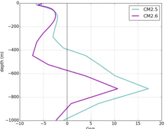
In the subsurface [;(200–2000 m)], both models show salt convergence by transient eddies peaking around 800-m depth (red lines inFig. 9). In CM2.6, eddy-driven salt convergence is around 2.5 times stronger than in CM2.5. In addition, in CM2.6, the transient eddy com- ponent opposes the time-mean component (blue lines in Fig. 9). The eddy-driven salt convergence opposing the time-mean salt divergence corresponds to a restratifying effect by eddies. Transient mesoscale eddies are known to extract the available potential energy imparted by winds from the mean flow, leading to a restratification of the upper ocean characterized by a flattening of iso- pycnal surfaces (e.g.,Gent and McWilliams 1990;Gent et al. 1995;Su et al. 2014).
FIG. 7. Current speed (m s21; color shading) ands0isopycnals (kg m23; solid black lines) for (left) CM2.5 and (right) CM2.6 between 200-m depth and the ocean bottom of the Weddell Sea region averaged over years 106 to 125. The solid red lines correspond tos0isopycnals averaged over years 1 to 20 of the simulations and are only shown at the eastern and northern boundaries of the domain for clarity. Isopycnals range from 27.72 to 27.85 kg m23 with a 0.01 kg m23contour interval and are masked on the continental shelf (i.e., regions shallower than 1000 m).
The thick green line indicates the 1000-m isobath that separates the open-ocean from the continental shelf.
Between 200 and;1000 m, the sum of the time-mean and eddy components results in salt advection di- vergence for CM2.6 and convergence for CM2.5 (black lines in Fig. 9). Similarly to heat advection, salt
advection is mainly balanced by vertical mixing below 200 m with a small contribution from the submesoscale parameterization (seeFig. 4). Depending on the years analyzed, the resulting total salt tendency is positive or
FIG. 9. Salt convergence [Gg s21;1023Sv (1 Sv[106m3s21)] due to advection in the open-ocean region of the Weddell Sea (i.e., regions deeper than 1000 m; seeFig. 1) for years 181–184 in (left) CM2.5 and (right) CM2.6 below 200 m. The total advection (black dashed line) is decomposed into a time-mean component (blue plain line) and a transient eddy component (red plain line). For details on the decomposition, the reader is referred tosection 4c(1).
Positive values indicate salt convergence.
FIG. 8. Time series of yearly (a) surface heat fluxes, (b) freshwater fluxes, and (c) buoyancy fluxes in the open-ocean region of the Weddell Sea (i.e., regions deeper than 1000 m; seeFig. 1) for CM2.5 (cyan) and CM2.6 (magenta). Positive values indicate a flux into the ocean. The vertical dashed lines indicate the two time periods discussed insection 4b(2), respectively, years 106 to 125 and years 161 to 180. The gray shadings correspond to the time periods of the two polynya events in CM2.6.
negative, as reflected by the inflation and deflation of the salt reservoir over the course of the simulation (Fig. 3).
In contrast to CM2.6, the time-mean component of CM2.5 converges salt between 200 and 2000 m, hence conspiring with the eddy component. The resulting total advective component is balanced by a strong vertical mixing that acts to erode the salt reservoir (not shown), thus weakening the stratification.
Salt is advected into the open-ocean region of the Weddell Sea through the gyre circulation and the off- shore transport across the shelf break. The maximum of salt transport across the eastern and northern bound- aries of the Weddell Sea is found to be consistently shallower by ;300 m in CM2.5 than in CM2.6 (not shown), leading to a shallow convergence of salt in CM2.5. This shallower salt transport in CM2.5 might arise from a weaker gyre circulation, illustrated by a weaker and shallower ASC in CM2.5 (Fig. 7). In addi- tion, salt from the continental shelf is found to be transported offshore at shallower depth in CM2.5 than in CM2.6, also contributing to a shallower convergence of salt in the open-ocean region in CM2.5. Figure 10 shows the time-mean component of salt transport across the continental shelf boundary in the two models. Off- shore salt transport is found as shallow as 400-m depth in CM2.5, while it is found to occur below;580-m depth in CM2.6. In addition, offshore salt transport is stronger in CM2.5 than in CM2.6, most likely due to higher sa- linity on the shelf in CM2.5 (10.11 psu). In the follow- ing, we argue that the shallow offshore salt transport in CM2.5 is related to a drastic lack of dense water over- flows. Rather than cascading down the continental slope to the deep Weddell Sea, the dense, saline waters
formed on the continental shelf tend to mix at shallow depths due to CM2.5’s coarser horizontal resolution.
2) EFFECT OF OVERFLOWS ON STRATIFICATION
Figure 7compares the density structure between years 1–20 and years 106–125 in CM2.5 and CM2.6. Both models are initialized from the same fields (see section 2a).
However, as each model has its own dynamical adjust- ments from the beginning of the simulations, the density structure of years 1–20 of CM2.5 and CM2.6 show signif- icant differences. Over time, CM2.5 shows a large down- ward displacement of isopycnals along the continental slopes compared to CM2.6, corresponding to a dramatic collapse of the density structure. For instance, the in- tersection of the 27.83 isopycnal height with the conti- nental slope at the eastern boundary of the Weddell Sea drops by around 1100 m over 105 years in CM2.5 (Fig. 7).
This drift in isopycnals over the continental slopes is re- duced by a factor of 2 in CM2.6. The volume of densest waters inFig. 7, which is contoured by the 27.85 isopycnal and encompasses the AABW, shrinks in both models. By years 106–125, it has almost disappeared in CM2.5.
Using the ocean model OCCAM at the same resolu- tion as CM2.5,Lee et al. (2002)found a similar large downward displacement of dense isopycnals in the Southern Ocean sector of their simulations (see their Fig. 3). The rate of isopycnal displacement in their model is on the order of 35 m yr21, greater than that found in CM2.5 (order of 10 m yr21). Attributing the difference in the rates of displacement between CM2.5 andLee et al.’s (2002) model is difficult owing to the numerous differences between the two models. Simi- larly,Dufour (2011)reported a downward displacement of dense isopycnals in the Southern Ocean in the ocean model NEMO, run at the same resolution as CM2.5.
This displacement of isopycnals was associated with a doming of isopycnals as seen in CM2.5 (see Dufour 2011, p. 54, Fig. 2.1) and with a volume loss of AABW of 25% in 46 yr of simulation.Lee et al. (2002)andDufour (2011) interpreted the vertical displacement of iso- pycnals as a consequence of both a lack of resupply of AABW to the abyssal ocean and an enhanced con- sumption of AABW by spurious mixing processes.
Similarly, in CM2.5, we attribute the collapse of strati- fication over the continental slopes of the Weddell Sea to weak overflows of dense waters off the continental shelf and intense erosion of AABW properties. Though also present in CM2.6, the collapse of stratification over the continental slopes is clearly weaker than in CM2.5.
The role of spurious mixing processes in eroding AABW will be briefly discussed insection 5.
Figures 11a–dshows4and oxygen (O2) at the ocean floor in the two models. Here,s4is preferred tos0ors2 FIG. 10. Time-mean component of salt transport [Gg s21;1023Sv
(1 Sv[106m3s21)] across the 1000-m isobath for years 181–184 in CM2.5 (cyan) and CM2.6 (magenta). Positive values indicate offshore transport.
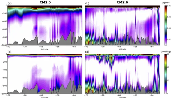
FIG. 11. (left) CM2.5 and (right) CM2.6: (a),(b)s4(kg m23) and (c),(d) O2(mmol kg21) at the ocean floor averaged over years 106–125 (color shading), 500-, 600-, and 700-m isobaths (thin gray lines), and 1000-m isobath (thick black line). The dashed black box in (a),(b) shows the western side of the Weddell Sea, on whichFig. 12 focuses. The 1000-m isobath shows the separation between the open ocean and the continental shelf. (e),(f) Cross-shelf section of O2(color shading;mmol kg21) and vertical velocity (white contours; m s21) at 66.58S averaged over years 106–125. White contours indicate velocities ranging from2531024to2231024m s21with a 131024m s21contour interval. Black boxes show close-up views of the topographic sill (dashed contoured region).
Note that the longitude range is different in (e),(f) and that depth only extends to 2000 m.
to assess the dense shelf waters’ ability to overflow to the deep ocean. In the models, dense ventilated waters are mostly formed on the southwestern corner of the con- tinental shelf of the Weddell Sea. From there, they spread to the northeast, as well as along the Antarctic Peninsula, while mixing with ambient waters. In contrast to high-s4waters, high-O2waters are also found in the Filchner Depression [;(308–458W)] in CM2.5. Other locations of high-O2waters are found east of 308W in both models. Possible causes of insufficient overflow transport are a lack of formation of dense waters on the continental shelf and/or a lack of representation of processes associated with downslope flows of dense waters in the model. In both models, dense waters formed in the southwestern corner of the continental shelf are of similar density as waters in the abyssal open- ocean region ($46.1 kg m23;Figs. 11a,b), thus showing they are dense enough to overflow to the deep ocean. In addition, CM2.5 simulates greater sea ice formation on the continental shelf (110%) as well as denser waters (10.092 kg m23) than CM2.6, suggesting that the density of shelf waters is not the main cause of weaker overflows in CM2.5 relative to CM2.6. Hence, shelf water density is unlikely the main cause of weak overflows in the models, nor is it the main cause of the differences in overflows between the two models. In the following, we
will focus on the difference in the representation of downslope flows of dense waters between the two models.
To visualize how dense ventilated waters outflow from the continental shelf, we present a cross-shelf section of O2 concentration and vertical velocity contours at 66.58S, averaged over years 106–125, inFigs. 11e,f. O2 concentration is the highest between the surface and
;200-m depth. Below 200-m depth, O2concentration is low in the open ocean and medium to high on the shelf.
At the shelf break, CM2.5 shows high O2concentrations but weak vertical O2 gradients and no downslope ve- locity on the offshore side of the shelf break (close-up view ofFig. 11e). In contrast, CM2.6 shows a tongue of high-O2 waters flowing over the topographic sill and downslope down to;1100 m (close-up view ofFig. 11f).
Figure 11fand analyses of the horizontal velocity com- ponents (not shown) suggest that the high-O2 slope current observed in CM2.6 corresponds to overflows that spill out of the shelf and flow along the continental slope while progressively crossing isobaths. In CM2.5, the same analysis suggests the absence of overflows;
rather, high-O2waters flow along the shelf break and get mixed across the ASF.
Figure 12 completes this view by presenting the standard deviation over years 181–184 for s0 and O2
FIG. 12. (left) CM2.5 and (right) CM2.6: zoom on the western side of the Weddell Sea indicated inFig. 11.
Standard deviation of (a),(b)s0(kg m23) and (c),(d) O2concentration (mmol kg21) along the 1000-m isobath.
Standard deviations are calculated from 5-day averages over years 181–184. Because topography is discrete in the model and topographic slopes are steep in many locations at the continental shelf, the algorithm that computes the 1000-m isobath from the model captures the ocean depth equal to 1000 m or the closest ocean depth shallower than 1000 m. Hence, the resulting topography (in gray) does not perfectly follow the 1000-m isobath; rather it is an approximation.
presence of pulses of dense, highly ventilated waters across the shelf break. We note that the locations of these hot spots are in agreement with locations of overflows reported from hydrographic data (e.g.,Baines and Condie 1998;Ivanov et al. 2004;McKee et al. 2011).
The finer horizontal resolution of CM2.6 relative to CM2.5 results in a better representation of topographic features (Figs. 11a–d and Fig. 12) and of the overflow process itself. In CM2.6, the edge of the continental shelf running along the Antarctic Peninsula displays small seamounts that show up as low-density and O2-poor water patches and deep narrow channels that show up as high- density and O2-rich water patches (658–728S;Fig. 11d). In between the seamounts, small channels can steer dense ventilated waters toward the edge of the shelf. Topo- graphic features such as canyons, troughs, and seamounts are known to play an important role in steering and channeling dense waters downslope, thus enhancing the overflows (e.g.,Wåhlin 2002). In CM2.5, a preferred route for dense high-O2waters out of the continental shelf is northward along the Antarctic Peninsula (Fig. 11c). In addition, CM2.6’s finer horizontal resolution reduces nu- merical entrainment in overflows that leads to excessive spurious mixing impeding the downslope flow of dense waters (Winton et al. 1998;Legg et al. 2006).
In this section, we showed that CM2.6 better repre- sents overflows than CM2.5. In the real world, dense waters that spill off the continental shelf cascade down the continental slope while undergoing some mixing with ambient water and eventually fill the abyssal ocean (e.g.,Foster and Carmack 1976). In CM2.5 and CM2.6, however, we find that dense waters that form on the continental shelf are unable to flow down to the abyssal ocean (Figs. 7and11). No evidence of dense water flows reaching depths greater than ;1500 m was found in either model. Rather, dense waters formed on the con- tinental shelf almost entirely mix with ambient open- ocean waters at intermediate depths across the ASF (see Fig. 10). Though this mechanism occurs in both models, the saline shelf waters from CM2.5 are injected signifi- cantly shallower in the water column than in CM2.6.
As a result, in CM2.5, the shallow mixing of the saline shelf waters contributes to a salinity bias in the upper
5. Discussion
a. Role of ocean mesoscale and overflows in the stratification of the Weddell Sea
The buildup of the subsurface heat reservoir in the Weddell Sea is a necessary condition for the formation and maintenance of a polynya in the open ocean. Using two climate models with oceans at different eddying resolutions, we found that the stratification in the open- ocean region of the Weddell Sea is key to the buildup of the subsurface heat reservoir. This study identifies two major drivers of the stratification in this region. First, the transient mesoscale eddies act to restratify the water column, thus reducing the doming of isopycnals in the Weddell Sea (Fig. 13a). The literature on the stratifica- tion control effected by mesoscale eddies in the ocean is abundant (for a review, seeMarshall and Schott 1999;
McWilliams 2008). Several studies have discussed more particularly the role of such eddies in the circulation of the Weddell Sea (e.g.,Newsom et al. 2016;Stewart and Thompson 2015;Su et al. 2014;Thompson et al. 2014).
But to our knowledge, none of these studies have re- ported on the contribution of mesoscale eddies to the stratification of the open-ocean region in the Weddell Sea. We note that our results are consistent with what is found in other regions, in particular in the Antarctic Circumpolar Current where the role of eddies in flat- tening isopycnal surfaces has been well documented (e.g., Gent and McWilliams 1990; Gent et al. 1995;
Marshall and Speer 2012). Second, the dense overflows that spill off the continental shelf of the Weddell Sea help support the stratification in the open ocean (Fig. 13b). Analogous results were found in the Labra- dor Sea where Yeager and Danabasoglu (2012)com- pared two versions of the CCSM4 model with and without an overflow parameterization [Snow et al.
(2015) looked at similar questions in the Southern Ocean]. They noted an enhancement in stratification when overflows are parameterized, with this enhance- ment in stratification inhibiting winter deep convection.
Fully resolving the ocean mesoscale spectrum in the open-ocean region of the Weddell Sea requires a
resolution as fine as1/258(e.g.,Hallberg 2013), as the first baroclinic deformation radius decreases with latitude.
Hence, CM2.6 (0.18 ocean) only partially resolves the ocean mesoscale spectrum in the Weddell Sea. Likewise, CM2.6 only partially resolves dense water overflows.
Winton et al. (1998)showed that resolution on the order of 3–5 km in the horizontal and 30–50 m in the vertical are needed to represent overflows inz-coordinate models. At the continental shelf break, CM2.6’s resolution is on the order of 5 km in the horizontal and 100 m in the vertical, which makes it too coarse to adequately resolve over- flows. Nonetheless, the comparison between CM2.5 and CM2.6 elucidates the role of transient mesoscale eddies and overflows in the stratification of the open-ocean re- gion of the Weddell Sea. Though a weakening in strati- fication occurs in both CM2.5 and CM2.6 from the initial state (Fig. 7), the stratification remains much stronger in CM2.6 than in CM2.5 because both mesoscale eddies and overflows are better resolved in CM2.6 (section 4c). As a result, the stratification remains strong enough in CM2.6 to allow the buildup of the subsurface heat reservoir, in contrast to CM2.5.
b. Other contributors to the stratification
Other processes may significantly influence the strat- ification of the Weddell Sea. In the following, we briefly discuss two other possible contributors to the difference in stratification between CM2.5 and CM2.6, namely spurious diapycnal mixing in the ocean interior and dense shelf water formation.
High rates of diapycnal mixing can arise from spurious diffusion associated with tracer advection schemes (e.g.,
Griffies et al. 2000). Such spurious diapycnal mixing is typical ofz-coordinate models where truncation errors can be large depending on the advection scheme used (e.g.,Griffies et al. 2000;Ilıcak et al. 2012). CM2.5 and CM2.6 use the multidimensional piecewise parabolic method (MDPPM; Griffies 2012), with flux limiters based onSuresh and Huynh (1997), for advecting ocean tracers. The MDPPM is one of the advection schemes based on higher-order approximations, thus limiting implicit diffusion. However, despite the use of higher- order advection schemes and the decreasing rate of spurious diapycnal mixing with increasing resolution, significant spurious diapycnal mixing can still persist in eddying models (Urakawa and Hasumi 2014).Lee et al.
(2002)reported a rapid drift of AABW properties from the model initial state due to spurious diapycnal mixing in 0.258ocean simulations. In our models, the volume of AABW properties is found to significantly shrink over the course of the simulation, with a reduced shrinking in CM2.6 compared to CM2.5 (Fig. 7). This shrinking suggests some spurious diapycnal mixing with overlying waters, thus eroding AABW thermohaline properties.
As the finer resolution of CM2.6’s ocean component should lead to reduced truncation errors, we infer higher rates of spurious diapycnal mixing in CM2.5 than in CM2.6. These higher rates of spurious diapycnal mixing are likely to be one of the contributors to the weaker stratification of the open-ocean region of the Weddell Sea simulated in CM2.5.
The formation of dense waters on the continental shelf mainly occurs within coastal polynyas that strongly depend on atmospheric conditions, in particular on
FIG. 13. Summary schematics of the contributions of transient mesoscale eddies and dense water overflows to the open-ocean stratification. (a) Transient mesoscale eddies induce a flattening of isopycnals and thus act to restratify the water column. (b) In the real world, dense waters formed on the continental shelf spill off the shelf through overflows and descend along the continental slope while mixing with ambient water. In our models, dense shelf waters are unable to reach the abyssal ocean. Rather, these waters mostly mix with ambient waters at middepth. In CM2.5, this mixing occurs at a significantly shallower depth than in CM2.6, thus causing an increase in salinity in the upper ocean that eventually weakens the stratification.
suffer from a lack of dense shelf water formation. We note that CM2.5 shows greater sea ice formation and forms denser waters on the continental shelf than CM2.6 [see section 4c(2)]. These results are in contrast with that from Newsom et al. (2016), who found dense shelf water forming at higher density in a 0.108climate model than in its 18counterpart. However, their 18climate model pa- rameterizes mesoscale eddy transport contrary to our 0.258CM2.5 model, thus precluding the interpretation of the differences between our results. In contrast to our model, the 0.108 model used by Newsom et al. (2016) shows high formation rates and export of dense shelf waters that could possibly explain the absence of large Weddell Sea polynyas in their model (Martinson 1991).
6. Summary
A necessary condition for the formation and mainte- nance of open-ocean polynyas in the Weddell Sea is the buildup of the subsurface heat reservoir, which is tied to the stratification. In this study, we investigate which processes help maintain the stratification in the Weddell Sea, hence allowing for the buildup of the subsurface heat reservoir. To do so, we use two climate models of different eddying resolutions in the ocean. We find the following:
d The higher-resolution model (CM2.6; 0.18in the ocean) simulates two large polynyas over the course of the simulation. In contrast, the coarser-resolution model (CM2.5; 0.258in the ocean) does not simulate any large polynyas; rather, it features quasi-continuous deep convection that erodes the subsurface heat reservoir.
Deep convection is thus found to be an insufficient condition for the occurrence of a polynya.
d In CM2.5, the quasi-continuous deep convection is due to enhanced vertical mixing between the surface and subsurface. Enhanced vertical mixing is triggered by episodes of gravitational instabilities associated with weak stratification. The stratification is in turn weakened by the deep convection. The weak stratifi- cation shows up as an increased doming of isopycnals in the open-ocean region of the Weddell Sea. In
stratification of the open ocean (Fig. 13b). The stron- ger stratification of CM2.6 compared to CM2.5 is due to a better representation of both processes. The finer ocean grid of CM2.6 leads to enhanced resolution of transient mesoscale eddies and to reduced spurious numerical entrainment of dense waters and better resolution of topographic features (such as canyons, troughs, and seamounts) that are both key to the representation of overflows.
While the role of surface forcing on stratification has attracted the most attention so far, our results reveal that interior ocean processes, such as transient meso- scale eddies and deep overflows, are important for the Weddell Sea stratification. However, to quantify their respective roles in the Weddell Sea stratification, dedi- cated sensitivity experiments would be required. If not explicitly resolved in climate models, these processes should be parameterized.
Acknowledgments.C. O. Dufour was supported by the National Aeronautics and Space Administration (NASA) under Award NNX14AL40G and by the Princeton Envi- ronmental Institute (PEI) Grand Challenge initiative.
A. K. Morrison was supported by the U.S. Department of Energy under Award DE-SC0012457, by the PEI Grand Challenge initiative, and by the Australian Research Council DECRA Fellowship DE170100184. I. Frenger was supported by the Swiss National Science Foundation Early Postdoc Mobility Fellowship P2EZP2-152133 and NASA under Award NNX14AL40G. This work was performed in J. L. Sarmiento’s team at Princeton Uni- versity. The Southern Ocean Carbon and Climate Obser- vations and Modeling (SOCCOM) project, supported under the National Science Foundation Award PLR- 1425989 and led by Sarmiento, provided a favorable en- vironment and some travel support for this work. We thank Robert Hallberg, Sonya Legg, and Gustavo Mastrorocco Marques for helpful comments and in- sightful discussions on this manuscript. We also thank Miguel Morales Maqueda and two anonymous reviewers for providing sound and constructive comments that greatly improved this manuscript.