2.Study area

(1)

Bachelorarbeit

Zur Erlangung des akademischen Grades Bachelor of Science Thema der Arbeit:

Thermokarst lake dynamics on the Alaska North Slope and their influence on organic matter deposition

eingereicht von: Linda Siegert Matrikelnummer: 582443

E-Mail: siegertl@hu-berlin.de

Gutachter/innen: Prof. Dr. Christoph Schneider Dr. Josefine Lenz

Eingereicht am Geographischen Institut der Humboldt-Universität zu Berlin am 30.07.2019

(2)

Bachelor´s thesis

To earn the academic degree Bachelor of Science

Topic of the thesis:

Thermokarst lake dynamics on the Alaska North Slope and their influence on organic matter deposition

Photo: J.Lenz

Submitted by: Linda Siegert Matrikelnummer: 582443

E-Mail: siegertl@hu-berlin.de

Internal Supervisor: Prof. Dr. Christoph Schneider External Supervisor: Dr. Josefine Lenz

rd

(3)

Outline

Abstract 5

1. Introduction 6

1.1 Thermokarst lake development 7

1.2 Research hypotheses 8

2.Study area 9

2.1 Permafrost 11

2.2 Geology 12

2.3 Climate and vegetation 13

3.Methods 14

3.1 Field work 14

3.2 Laboratory work 15

3.2.1 Sample preparation 15

3.2.2 Total carbon and total nitrogen 16

3.2.3 Total organic carbon 16

3.2.4 Stable carbon isotopes 17

3.3 GIS analytics 18

3.3.1 Lake size 18

3.3.2 Grounded ice lakes and floating ice lakes 18

4.Results 19

4.1 Field work 19

4.2 Laboratory work 19

4.2.1 Core descriptions 19

4.2.2 Total carbon and total nitrogen 21

4.2.3 Total organic carbon 22

4.2.4 Stable carbon isotopes 22

4.3.1 Lake size 23

4.3.2 Grounded and floating ice lakes 24

5. Discussion 25

5.1 Interpretation of organic matter characteristics 25

5.3 Work Hypotheses 27

5.3.1 First work hypothesis 27

5.3.2 Second work hypothesis 28

5.3.3 Third work hypothesis 30

6. Outlook 31

7. Conclusion 31

8. Attachment 32

9.Appendix 35

Tables of data 35

(4)

List of Figures

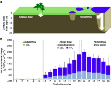
Figure 1: Difference of gradual and abrupt thawing (Walter Anthony et al. 2018) 6 Figure 2: Thermokarst lake development in five stages (Grosse et al., 2013) 7

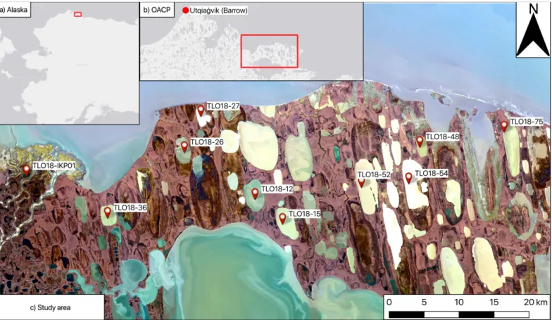
Figure 3: Spatial classifying of the study area 9

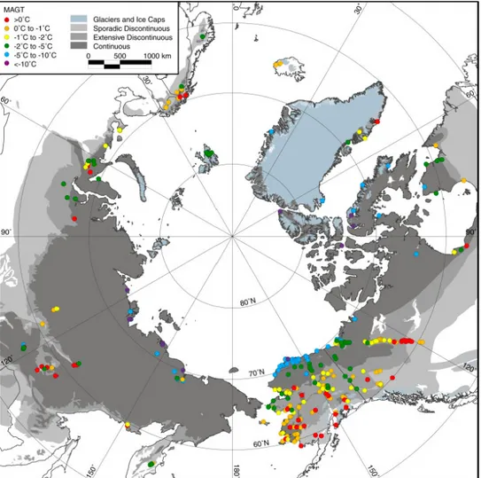
Figure 4: Permafrost classifications and permafrost temperatures (Romanovsky et al. 2010) 11

Figure 5: Bedrock geology – Alaska (Woodward et al., 2011) 12

Figure 6: Climate chart of Barrow, Alaska from 1987 to 2016 (NOAA) 13

Figure 7: Core taking on a float boat with a piston corer 14

Figure 8: Electrical Conductivity of lakes 19

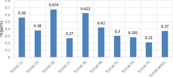
Figure 9: Total nitrogen of all cores 21

Figure 10: Total carbon of all cores 21

Figure 11: Total organic carbon in all cores 22

Figure 12: Stable carbon isotopes ratio of all cores 22

Figure 13: Lake size dynamics of Lakes 26, 27, IKPO1 and 75 23

Figure 14: Lake size dynamics of lake 52, 54, 48, 36, 12 and 15 24

Figure 15: Study area with grounded and floating ice lakes 24

Figure 16: C/N ratio of all cores 25

Figure 17: C/N ratio and δ13C values of all cores 26

List of Tables

Table 1: Core and lake conditions during field work 10

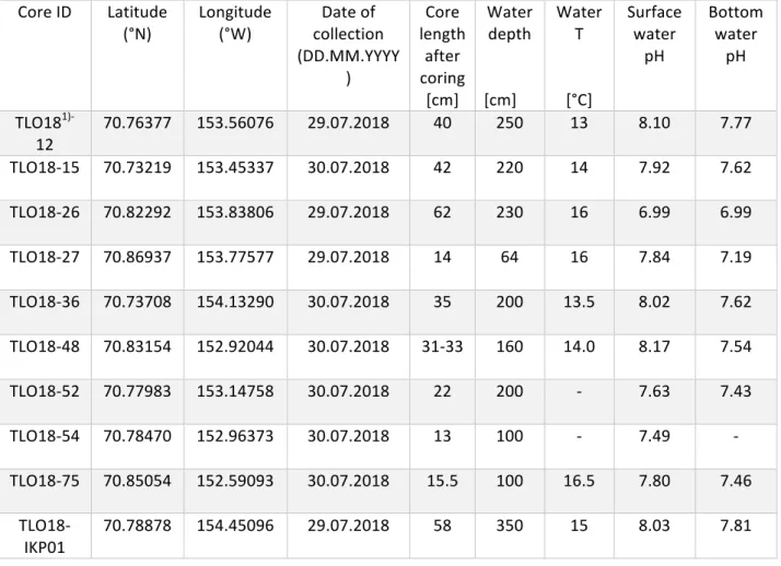
Table 2: Core descriptions 20

Table 3: Lake dynamics (size changes) from 1986 to 2018 23

Table 4: Summarised results for the first work hypothesis 28

Table 5: Summarised results for the second work hypothesis 29

Table 6: Summarised results for the third work hypothesis 30

(5)

Abstract

Arctic regions are affected by the warming twice times faster than the global mean. (Overland et al., 2017) Within the last years permafrost has rapidly thawed which is a significant issue in relation to climate change and landscape structures in arctic regions.

The biggest issue of rapidly thawing permafrost are the stored carbon sources in the ground which contain a lot of methane and carbon dioxide. Thus climate change is a lot influenced by self-enforcing feedback effects which have a very high impact (Pithan et al., 2014).

This study is based on 10 short sediment cores taken from thermokarst lakes on the Alaska North Slope in July and August 2018 by researchers of the Alfred Wegener Institute for Polar and Marine Research and the University of Alaska Fairbanks.

The main focus of this thesis is the understanding of the dynamics of thermokarst lakes based on geochemical analyses, physical parameters and remote sensing imageries.

Within this study the dynamics of thermokarst lakes were discussed and researched in relation to their decomposed organic matter content.

The relation between the lake size, water depth, lake ice type and organic matter input was discussed as well.

Lastly this thesis canvased the influence of salinity of organic matter input.

The method of these classifications is qualitative and is handled by data tables without statistical classifiers.

(6)

1. Introduction

The northern part of Alaska, namely the Alaskan North Slope, is characterized by arctic conditions in all categories. It is especially influenced by continuous permafrost. Permafrost is vulnerable to climate change and as a consequence of increasing air temperatures thawing processes create visible changes in the landscape because of the resulting increased ground temperatures as well (Romanovsky et al. 2010).

An obvious evidence for thawing processes and the resulting degradation of permafrost are thermokarst lakes.

These types of lakes are very complex in their development and very relevant on a global level since they act as carbon sinks or carbon sources and even provide information about the global greenhouse gas emissions according to their state of development. (Walter et al. 2007) The velocity of thawing is very significant according to the release of greenhouse gases. Abrupt thawing causes more degassing of carbon dioxide (CO2) and especially methane (CH4) than gradual thawing over years (Figure 1).

It is also necessary to realize that the lakes start to freeze every autumn and thaw every spring.

In relation to the cycle of the seasons the albedo changes as well. If the thawing processes are advantaged more through increasing temperatures, the annual albedo is higher which means a self-enforcing feedback effect. So it is very important to study the dynamics of the lakes to provide information about the impacts of the climate change in relation to permafrost thawing processes. Deposited sediments of the lake ground can also give a view on the variability of the environment during the Holocene. (Lenz et al. 2016)

Figure 1: Difference of gradual and abrupt thawing. a schematic, b Net ecosystem exchange in Greenland (1,2), Healy, Alaska (3-5), western Alaska (6-9), interior Alaska (10, 11, 14-19), northeast Siberia (12, 13), (Walter Anthony et al. 2018)

(7)

1.1 Thermokarst lake development

The periglacial landscape is characterized by ice-rich permafrost and ice wedges.

Thermokarst lakes develop by ground ice loss, ground subsidence and pooling of water. That is why the natural rhythm of summer and winter is important by the development of thermokarst lakes, too. The active layer of the permafrost starts to thaw at the beginning of summer and starts to freeze at the end of the late summer.

The abrupt thawing causes visible bulges in the landscape (Figure 2 (b)). The thawing causes a depression which gets filled by thawing waters and precipitation waters (Figure 2(c)). Ice wedges accelerate these processes because of the ice-richness which indicates more thawing waters. (Figure 2 (d)). Ice wedges also cause degrading in a much more intense way at the places where they developed. As ice wedges develop in a high amount in arctic tundra, the occurrence of them is very significant. The non-frozen Talik also causes thawing around the lake because of the heat flux in direction to the surrounding permafrost (Figure 2 (e)), Grosse et al., 2013).

(8)

1.2 Research hypotheses

The main focus of this bachelor´s thesis project will be the analyses of the relationship between the lake type characteristics and organic matter deposition of lake sediments based on 10 short sediment cores with references to their dynamics.

One category of the lake classification will be dynamic and stable lakes. For this category comparison of remote sensing imageries will be used to get an idea of the lake size changes over the past 32 years. It is also expected that the stable lakes consist of more decomposed organic matter than the more dynamic lakes because they tend to change in size more often which is a reason for a higher rate of terrestrial plants than aquatic plants. It is expected as well that larger and deeper grounded ice lakes contain less organic matter input and rather feature aquatic plants than smaller and shallower floating ice lakes.

Marine influenced and freshwater lakes will be studied to get an idea of the organic matter in relation to their salinity.

Consequently, the three main research hypotheses are:

1. Sediments of stable lakes comprise more organic matter decomposed and rather aquatic plants than dynamic lakes which may contain less organic matter decomposed and rather terrestrial plants.

2. Sediments of smaller, shallower, grounded ice lakes have a lower organic matter input than larger, deeper, floating ice lakes.

3. Lakes with higher salinity provide a lower organic content than lakes with lower salinity.

(9)

2.Study area

The study area extends from 70.4° to 70.9° N latitude and from -152.2 to -154.5° W longitude (Figure 3).

The region is in the North of Alaska on the Alaska North Slope and is also partly located on the Outer Arctic Coastal Plain (OACP). Thus, this area is influenced by marine waters.

Especially the north coast of Alaska is influenced by a very fast coastal erosion which

influences the salinity and drainage of thermokarst lakes as well. In a span of 1955-2005 the coast has eroded up to 0.9 km at some points in the north of Teshekpuk lake (Mars et al, 2007).

22.5 % of the OACP are covered up with thermokarst lakes and 61.8 % of the landscape are drained thermokarst lake basins. (Jones et al., 2015)

Figure 3: Spatial classifying of the study area, a) Study area (red) marked at the North of Alaska, b) Study area (red) marked on OACP, c) Concrete study area with taken cores, (Backmap a) and b) from Esri (Copyright © Esri), c) Landsat 8 satellite imagery provided by USGS Data Center)

(10)

Ten cores were taken on 29^th and 30^th of July in 2018. Every core was taken from a different lake. The core length was measured right after coring.

Water depths and water temperatures were measured as well. The water depths reach up from 67 cm to 350 cm which shows a variability of lake depths.

Water temperatures are very similar from 13 °C to 16.5 °C.

Surface water pH values and bottom water pH values were measured to analyse the water quality of the lakes. They reach from a minimum of 6.99 to a maximum of 8.17. (Table 1) Pure water has a pH value of 7 which means that the lakes have no acidic properties. They rather tend to be more basic which means the lake waters contain more free hydroxyl ions.

Basic pH values in lake waters can be found because of a higher biotic productivity. (Institut Dr. Flad)

1) TLO18 denote Teshekpuk Lake Observatory 2018

Table 1: Core and lake conditions during field work

Core ID Latitude

(°N) Longitude

(°W) Date of collection (DD.MM.YYYY

)

Core length

after coring

[cm]

Water depth

[cm]

Water T

[°C]

Surface water

pH

Bottom water

pH

TLO18^1)-

12 70.76377 153.56076 29.07.2018 40 250 13 8.10 7.77

TLO18-15 70.73219 153.45337 30.07.2018 42 220 14 7.92 7.62 TLO18-26 70.82292 153.83806 29.07.2018 62 230 16 6.99 6.99 TLO18-27 70.86937 153.77577 29.07.2018 14 64 16 7.84 7.19 TLO18-36 70.73708 154.13290 30.07.2018 35 200 13.5 8.02 7.62 TLO18-48 70.83154 152.92044 30.07.2018 31-33 160 14.0 8.17 7.54 TLO18-52 70.77983 153.14758 30.07.2018 22 200 - 7.63 7.43

TLO18-54 70.78470 152.96373 30.07.2018 13 100 - 7.49 -

TLO18-75 70.85054 152.59093 30.07.2018 15.5 100 16.5 7.80 7.46 TLO18-

IKP01 70.78878 154.45096 29.07.2018 58 350 15 8.03 7.81

(11)

2.1 Permafrost

Permafrost is classified as a

The landscape is marked by the influence of the continuous ice-rich permafrost up to thicknesses of minimum 410 m (Jorgenson et al. 2008).

The temperatures of the permafrost are cold with mean annual values of -6 to -10 °C (Figure 4, Romanovsky et al. 2010). Hence this region consists of a lot of thermokarst lakes because of the thawing processes caused by summertime temperatures and because of the intensified feedback effect by the climate change (Pithan et al., 2014).

Figure 4: Permafrost classifications and permafrost temperatures (Romanovsky et al. 2010)

(12)

2.2 Geology

The geology of the surface is composed of Late Quaternary marine and terrestrial deposits (Jorgenson et al. 2008).

The ice-rich marine clay, silt deposits, beach and deltaic sands are overlain by younger Pleistocene and Holocene terrestrial sediments in the parts of the OACP.

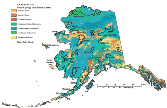
The bedrock geology of the study area is characterized by volcanic rocks around the Teshekpuk Lake area. The east part of the OACP consists of ancient marine sedimentary and the west part of continental sedimentary (Figure 5).

Figure 5: Bedrock geology – Alaska (Woodward et al., 2011)

(13)

2.3 Climate and vegetation

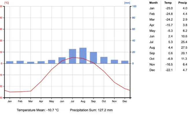
Figure 6: Climate chart of Barrow, Alaska from 1987 to 2016 (NOAA)

The study area is influenced by the arctic climate which is why there are annual mean air temperatures of -10.7 °C. The summer months are cool with a mean July air temperature of 5.3 °C in Barrow and winter months can get very cold with mean January air temperatures of -25 °C. There are very low precipitation rates in this study area of about 127.2 mm/a in average which indicates semi-arid conditions of the study area (Figure 6, Shulski and Wendler 2007).

The vegetation is mainly wetland vegetation with wet graminoids and moss. Because of the permafrost influence the landscape is dominated by high- and low-centered polygonal tundra (Nowacki et al. 2002). Especially because of the high amount of lakes in this area there is a high occurrence of lacustrine algae and marine algae in littoral parts as well.

(14)

3.Methods

3.1 Field work

The field work was conducted during an expedition of Alfred Wegener Institute for Polar and Marine Research (AWI) and also of the University of Fairbanks Alaska (UAF). It took place in July and August of 2018. This expedition was a part of the PETA-CARB project and was led by Prof. Dr. Guido Grosse (AWI, University Potsdam) and Dr. Benjamin Jones (UAF) based out of Teshekpuk Lake Observatory.

The main focus of the expedition was the submarine permafrost, the vegetation types in arctic tundra regions and also dynamics of thermokarst lakes.

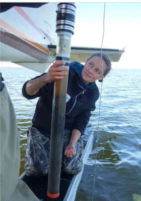
Dr. Josefine Lenz (AWI, UAF) drilled 10 cores from thermokarst lakes using a piston corer while standing on a float boat. (Figure 7) The lengths of the cores reach from 12 cm to 61.5 cm. It was cored until the frozen ground was reached which is why there was no ice contained in the cores. Every core was drilled from a different lake in order to assess spatial variability. The cores were almost always taken from the central of the lakes.

Lake depth, surface water temperature and electric conductivity were measured by Dr.

Josefine Lenz as well.

The cores were transported to AWI and were stored by 4 °C until November 2018 when they got opened.

Figure 7: Core taking on a float boat with a piston corer (Photo: Juliane Wolter)

(15)

3.2 Laboratory work

To ascertain the characteristics of the deposits of the lake ground in relation to carbon content, sediment compounds and vegetation classes the samples got analysed on a geochemical base. The cores were subsampled to determine the total carbon (TC), total organic carbon (TOC), total nitrogen (TN) and isotope ratio of total organic carbon (δ13C).

Besides the geochemical analyses the cores were described by their visual characteristics (amount of visible organic), their colour, their grain size and their size.

3.2.1 Sample preparation

The cores were cut in halves with an electronic saw. One half was used to archive each core and was stored isolated. The other half was used to get subsamples taken from it. The samples got taken with a syringe. This tool helped against a contamination of the samples under each other. The taken subsample was split in two 12.5 ml plastic jars (A and B sample) thus every sample was archived as well and the other part could be used for the geochemical analyses.

The studied core half was described visually before sample extraction. Every core was classified by its length, colour, grain size, organic matter content and structure. The colour was defined with the Munsell colour system by Albert H. Munsell. The grain size was conducted qualitatively with roll validations. The organic matter content was classified visually, as well as the structure of the cores.

The wet samples got weighted and were freeze-dried afterwards to extract the water.

The dried samples got milled with a Fritsch pulverisette 5 planetary mill to create a homogenous powdered sample. Each sample was milled in agate jars and agate marbles for 5 minutes at 360 rotations per minute and was transferred into plastic jars with a spatula and a brush.

For this study it was relevant to use the sample data of the first 10 cm averaged of each core.

This decision was made because there is no relation to a specific point of time since there was no radiocarbon dating measurement made. This is why there is a discussion about the lake classification at the end besides all other named work hypotheses.

(16)

3.2.2 Total carbon and total nitrogen

Every sample was measured twice for the analyses of TC and TN, which both could be determinate within one measurement. The amount of each sample weighted between 5 to 5.8 mg. The samples were weighted with a Sartorius micro M2P laboratory scale which has an accuracy of ± 0.001 mg. The samples were put in tin capsules and also Tungsten(VI)Oxide was added to catalyse the combustion process.

The vario EL III Elementar Analyzer (Elementar Analysensysteme GmbH) accomplished the measurement process. It heats the samples up to 950 °C with a helium atmosphere which is oxygen-saturated. At 850 °C the CO2, N2, NO and NO2 are formed and are reduced in a reduction tube.

The actual measurement begins at 50 °C which causes a mobilisation of nitrogen and a transfer to the measuring chamber. The nitrogen is getting detected by a heat conductivity sensor which appears as a peak in heat conductivity.

Afterwards, the vario EL III heats up to 130 °C again to begin the carbon dioxide transfer to the measuring chamber as well which causes another peak of heat conductivity. To prove the extent of the peaks it was important to put these into context with the sample weight.

Resulting values of TC and TN were given in wt% with an accuracy of 99.95 % for carbon and 99.9% for nitrogen.

It was necessary to prove these accuracies with calibration standards. Acetanilide, sucrose and 30 % EDTA were measured at the beginning of the set to control the set of standards used in between the sample measurements after every 30 measurements consisting of 20 % EDTA, 12 % calcium carbonate and two soil standards. Even the standards were measured twice and could have only a measurement difference maximum of 10 %.

3.2.3 Total organic carbon

It is important to distinguish total organic carbon from the total carbon content of the samples because the total carbon content also contains the inorganic carbon like little shell remains.

The total organic carbon was measured with the elementary analysis device varioMAX C Element Analyzer (Elementar Analysensysteme GmbH). It functions with catalytic tube pyrolysis while pure Nitrogen (99.996 %) is the carrier gas. The amount of the measured sample is based on its total carbon content. The samples were weighted with a Mettler Toledo XS105 dual range analysis scale with an accuracy of ± 0.1 mg) in steel crucibles.

(17)

At the beginning of the analysis, a set of calibration standards composed of pure glutamate, 30 % glutamate and 2:3 glutamate were used. After every 15 samples 2:3 glutamate, 10:40 glutamate, 5:45 glutamate and 1:19 glutamate were used to control the measurements.

The samples were heated up to 580 °C in a helium atmosphere which is oxygen-saturated to form them in carbon dioxide formation. To assure the complete carbon dioxide formation the gases were heated up to 930 °C. The device exhibits a detectable carbon content minimum of 0.1 %. The carbon dioxide peak during integration is determined by the cut off value which is calculated by sample mass and anticipated carbon amount. The total organic carbon content is defined by the value and arising of the peak. The accuracy of this method amounts to 99.9

%. Within the values of TOC and N there was calculated a ratio which implies the state of decomposition of the organic matter in the samples. The organic matter qualifies a better conserved state, if the values are higher.

3.2.4 Stable carbon isotopes

Carbon ions needed to be removed for stable isotope analysis. For this, a little amount of each sample was filled in Erlenmeyer glass flasks. Every sample was enriched with 20 ml 1.3 molar hydrochloride acid (HCl). The solution was heated up to 97.7 °C on a hot plate for three hours.

They were filled up with purified water afterwards. The samples were decanted every day for three days in a row to remove the Cl^- ions. It was necessary to reduce the Cl^-content of under 500 ppm. The elimination of these ions was needed to avoid disorders in the electromagnetic field of the mass spectrometry which is used for the measurements. Divergent ionization reacts could be avoid with this process as well. The samples were tested with Quatofix Chloride test stripes to ensure the amount of Cl^- ions in every sample.

The samples were vacuum-filtered, dried at 50 °C and hand-grinded afterwards to get the samples decarbonised and pulverised again.

The following equation shows the reaction while decarbonising the samples:

1.) "#_$^%&+ 2)"* → "#_% + 2"*^&+ )_%

To prepare the samples for the measurement it was necessary to weigh in a targeted amount of the samples with the following equitation:

2.),-./0, 102/ℎ, 4/ = ²⁰

(18)

The analysis was accomplished by Delta V Advantage Isotope Ratio MS supplement (Thermo Fisher Scientific) with a Flash 2000 Organic Elementar Analyzer (Thermo Fisher Scientific).

Both devices use helium as carrier gas.

The first step oft he analysis is the sample combustion and oxidationat 1020 °C with chrome dioxide as an oxidant which causes the formation of carbon dioxide (CO2) and pure nitrogen formations.

Elemental copper causes a reduction to pure nitrogen (N2) at 650 °C and leaves the CO2

unmodified. The gas chromatography tube separates the gases. Nitrogen comes into the mass spectrometry faster because its lighter than CO2. Inside the tubes, external nitrogen and external CO2 passes through the mass spectrometry to measure reference value. The measuring in general works by ionising the samples within electron impulses which are caused by energy inducing. The ions get separated by detection in the analysis unit where they get categorised by their mass and charge ratio and their energy intensity. The raw measured data has been calibrated to standards using a linear correction. The 1 σ standard error is better than ±0.15 ‰.

3.3 GIS analytics 3.3.1 Lake size

For lake size dynamics it was necessary to compare older stadiums with the latest situation of the lakes. Therefore, remote sensing images were used to compare the lakes size visually.

To find suitable images Google Earth Engine was utilised to find satellite images due the summer month. The cloud cover was filtered, too. As a result of this method, a Landsat 5 image from 12^th August 1986 and a Landsat 8 image of 19^th September 2018 were used to digitalise the lake outlines. The digitalisation was produced with QGIS3.6 and its polygon tool. Afterwards the lake size could have been ascertained with field calculator. For Lake IKPO1 there was only one suitable image from 25^th July 2006 available to show the dynamics of the lake properly.

3.3.2 Grounded ice lakes and floating ice lakes

The categorisation of grounded ice lakes and floating ice lakes was made with the assistance of scientific papers by Dr. Christopher D. Arp et al. from 2011 and 2012, hence these studies show already ascertained classifications for this study area.

(19)

4.Results

4.1 Field work

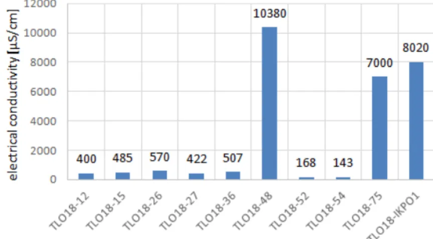
First results were made while field work. Important results of field work were the core taking and the measurement of electrical conductivity of the surface water.

The measured electrical conductivity of the surface water had a wide range of values between 143 µS/cm and 10380 µS/cm. (Fig.) The lakes 48, 75 and IKPO1 have the highest values with values between 7000 and 10380 µS/cm. The lowest values with 143 to 168 µS/cm were measured in the lakes 54 and 52. The remaining lakes have very similar values from 400 to 570 µS/cm.

4.2 Laboratory work 4.2.1 Core descriptions

The cores were described by their length, colour, grain size, organic matter content and structure (Table). The cores TLO18-27, -52, -54, -75 are the shorter cores of this study, they have a length of 12 cm to 22 cm. The longer cores TLO18-12, -15, -26, 36, -48 and -IKPO1 reach up from 32 cm to 61.5 cm. The cores spread from yellowish tones to reddish and brownish tones and also from lighter to black tones. The grain sizes reach from clay to sandy material.

Every core contains silt from fine to coarse. The cores TLO18-15, -36 and -48 contain coarser grain sizes up to fine sand and coarse silt. The other cores are more clayish and contained fine to middle silt.

TLO18-26, -36, -48 and -IKPO1 are organic dominated with visible organic remains, the others

Figure 8: Electrical Conductivity of lakes

(20)

Table 2: Core descriptions

Core ID Length

[cm] Colour

[Munsell, 1994]

Grain

size Organic matter

content Structure

TLO18-12 40 ^2.5Y

4/2, ->

2.5Y 3/1

fU to T fine organics at the end, lighter layers contain coarser organic

layering visible,

minerogenic dominated

TLO18-15 42 ^2.5Y

4/3 ->

5Y 3/2 ->

5Y 3/1

fS ->

gU->T visible organics at

the bottom minerogenic dominated

TLO18-26 61.5 ^5y

2.5/2 fU well decomposed,

coarser remains organic dominated, well layered

TLO18-27 13 ^5y

4/2 mU ->

T/fU no organic visible very minerogenic dominated, very dense

TLO18-36 36 ^5y

3/2 ->

5y 3/1

fU ->

gU well decomposed organic dominated, coarser minerogenic compounds at the bottom

TLO18-48 32 ^5Y

3/2 ->

black ->

5Y 3/1 ->

5Y 4/1

T/fU -

>

fU ->

gU ->

T

no organic visible at the top, macro organics visible in the middle

organic dominated, fine layered,

minerogenic at the bottom

TLO18-52 22 ^5Y

3/1 mU no organic visible very minerogenic dominated (silty), clay laminae

TLO18-54 12 ^2.5Y

4/2 ->

5Y 4/1

fU ->

T no organic visible very minerogenic dominated (clay), very dense

TLO18-75 16 ^2.5Y

2.5/1 ->

2.5Y 4/1

T to fU poorly

decomposed living vegetation at the top

minerogenic dominated, very dense

TLO18-IKPO1 57 ^2.5Y

3/3 ->

black ->

2.5Y 3/2 ->

2.5Y 2.5/1 ->

2.5Y 3/2 ->

black

mU larger remains, possibly aquatic, less-moderately decomposed

organic dominated

*-> = colour and grain size changes during core

(21)

4.2.2 Total carbon and total nitrogen

TC and TN values were measured in one measurement. The TN values are significant lower than the measured TC values. The values of TN and TC correspond with each other which shows a relation between total carbon and total nitrogen content. The TN values range between 0.21 wt% to 0.674 wt%. TLO18-12, -26 and 36 have the highest values with 0.56 wt%

to 0.674 wt%. The lowest values have been measured in TLO18-27, -54 and -75 with 0.27wt%, 0.281 wt% and 0.21 wt% (Figure).

The TC content is significantly higher and reach from 3.89 wt% to 11.487 wt%. The highest values were measured in TLO18-12, -26, -36 and -48. These values range from 7.04 wt% to 11.487 wt%. The lowest were measured in TLO18-27, -52, -54 and -75 with 4.35 wt%, 4.82 wt% , 4.5705 wt% and 3.89 wt% which is barely a third of the maximum (Figure).

Figure 9: Total nitrogen of all cores

(22)

4.2.3 Total organic carbon

The TOC values are in a very similar range (from 3.67 wt% to 11.337 wt %) as the TC values and correspond very well. The highest values were also measured in TLO18-12, -26 and -36.

Otherwise the lowest were measured in TLO18-27, -54 and -75 with 4.35 wt%, 4.5705 wt%

and 3.89 wt% again. TLO18-IKPO1 contains more TOC (5.23 wt%) than TC (5.11 wt%) (Figure 11).

4.2.4 Stable carbon isotopes

The δ13C values reach from -27.16 %VPDB to -29.52 %VPDB. The lowest values were measured in TLO18-IKPO1, -26, -36 and -12 which also describe the highest ratios. They spread between -28.68 %VPDB to -29.52 %VPDB. The highest values were measured in TLO18-27 and -75 with -28.3 %VPDB and -27.16 &VPDB which is a lower ratio of stable carbon isotopes (Figure 12).

Figure 11: Total organic carbon in all cores

Figure 12: Stable carbon isotopes ratio of all cores

(23)

4.3 GIS analytics 4.3.1 Lake size

The digitalisations of lake sizes show spatial variabilities over the years 1986 to 2018. (Table 3, Figure 13, 14) The most dynamics were visible on the lakes 27, 12 and 36. They register a size change of 7.18% to 5.82 %. The lowest changes were calculated on lake 75 with 0.25 % and lake 54 with 3.89 %. Every lake, except lake 27, register a positive lake size growth. The lake 27 shows a negative lake growth and implies a drainage.

Table 3: Lake dynamics (size changes) from 1986 to 2018

Lake ID Lake size 1986

[km²] Lake size 2018

[km²] Dynamic

[%]

12 ^9,844 ^10,485 ^0,641 ^6,11

15 ^9,572 ^10,018 ^0,446 ^4,45

26 ^6,449 ^6,723 ^0,274 ^4,08

27 ^4,028 ^3,758 ^-0,270 ^-7,18

36 ^5,535 ^5,877 ^0,342 ^5,82

48 ^3,809 ^3,987 ^0,178 ^4,46

52 ^18,524 ^19,505 ^0,981 ^5,03

54 ^16,727 ^17,404 ^0,677 ^3,89

75 ^13,035 ^13,068 ^0,033 ^0,25

IKPO1 ^0,652* ^0,689 ^0,037 ^5,37

*Lake size was digitalised with Landsat 5 image from 25th July 2006

(24)

Figure 14: Lake size dynamics of lake 52, 54, 48, 36, 12 and 15 (Backmap from Landsat 8 satellite imagery provided by USGS Data Center)

4.3.2 Grounded and floating ice lakes

There are several papers by Arp published which allow to classify the ice of the lakes in this study area. For most of the studied lakes there is used a classification of the lake ice regime classes from mid-April. It shows an Advanced Synthetic Aperture Radar imagery in the OACP from 2003 to 2011.

The lakes 27, 48, 54 and 75 are classified as grounded ice lakes. The lakes 12, 15, 26, and 52 (2007) were categorised as floating ice lakes. (Arp et al., 2012) Lake 36 is a floating ice lake as well. (Arp et al., 2011) For lake IKPO1 was no classification available. (Figure 15)

Figure 15: Study area with grounded and floating ice lakes (Data from Arp et al., 2011, Arp et al., 2012, Backmap from Landsat 8

(25)

5. Discussion

5.1 Interpretation of organic matter characteristics

Most of the made visual characterisation corresponds with the measured TOC content as well.

As TLO18-26, -36, -48 and –IKPO1 were classified as organic dominated, they also show the highest TOC contents. On the other hand, it is shown that TLO18-12 contains even more total organic carbon than TLO18-IKPO1 which was not suspected while describing the core because it was characterised as minerogenic dominated (Table 2).

As the results show, the carbon content of TC and TOC measurements are corresponding. The TOC in TLO18-IKPO1 is higher than the measured TC values. This represents that there is barely any inorganic carbon in this core. Higher inorganic carbon content would be shown as remains of shells or crustacean which is not a significant result of this study.

As TN values provide the bio productivity of each core. The cores TLO18-12, -26, -36 and -48 show values >0.4 wt% and >8.2 wt% TOC which indicates a higher bioproductivity (Lenz et al., 2013).

The C/N ratio shows shows the degree of decomposition (Figure 16), while the ratio of C/N and δ13C provide the discrimination of organic sources or vegetation origin (Figure 17, Lenz et al., 2016).

Figure 16: C/N ratio of all cores

(26)

Figure 17: C/N ratio and δ13C values of all cores

5.2 GIS analytics

The measured dynamic of the lakes was expected to occur mostly as a positive growth, which also happened as expected, because of the increasing ground temperatures. (Romanovski et al., 2010) On the other side, a lot of thermokarst lakes in this area lean to drain, thus there is resulting a high thermo-erosion in the ground (Jones et al., 2015).

It is also interesting to have a look on the growth direction because there is no growth in all directions. Lakes 12, 15, 26, 36, 48, 52, 54 and 75 all tend to expand in northern directions, thus they stretch to the coastal area. (Figure 13 and 14, Arp et al., 2011)

While studying the grounded and floating ice lakes, there showed a spatial distribution of every lake type. Grounded ice lakes seems rather to appear in the east part of the study area, while floating ice lakes seems to be rather in the centre and west of the study area.

(27)

5.3 Work Hypotheses 5.3.1 First work hypothesis

The analytical results were used to show how different lake parameter relate to each other.

First work hypotheses express an assumed relation between stable lakes, more decomposed organic and rather aquatic plant remains in comparison to dynamic lakes which contain less decomposed organics and rather terrestrial plants. To prove this hypotheses, it is necessary to prove if there are lake which show these assumed parameters at the same time. While Lakes 26, 48, 54 and 75 are classified as stable lakes. The lakes 12, 15, 27, 36, 52 and IKPO1 are categorised as dynamic lakes. To examine the rate of decomposed organics it is necessary to use the C/N ratio. It classifies the stable lakes 48, 54 and 75 as the most containing decomposed organic. However, the fourth stable lake 26 is classified containing the lowest decomposed organic material which does not fit to the assumed hypotheses and which is not suitable for the further proving. To verify the vegetation origin, it is necessary to show a relation between d13C values and C/N ratio. It shows that the stable lakes 48, 54 and 75 contain more decomposed organic and do not contain aquatic plants. The cores TLO18-48 and -75 contain terrestrial plants which shows clearly the opposite of the assumed hypothesis.

Even core TLO18-54 contains rather terrestrial plants. Otherwise, the other stable lake with less decomposed organic contains lacustrine algae. As a result of this, it could be said that stable lakes contain rather decomposed organic but it can not be proved that they also contain rather aquatic material which seems to depend on its decomposing level as well.

The dynamic lakes 12, 15, 27, 36, 52 and IKPO1 are assumed to contain less decomposed organic. This is accurate for lakes 12, 36 and IKPO1. Otherwise, TLO18-15, -27 and -52 show higher decomposition values which is then not suitable for further analytics in relation to first hypothesis. TLO18-12 contains rather lacustrine algae which is the opposite of the supposed hypotheses. TLO12-36 and IKPO1 contain rather terrestrial plants which is accurate in relation to the first hypotheses. The other dynamic lakes, which contain rather decomposed organics, contain rather terrestrial plants as well. All in all, the first hypotheses can not be confirmed because there are some contradictions and only two lakes are accurate.

(28)

Table 4: Summarised results for the first work hypothesis, Dynamic, C/N ratio and Vegetation origin

Core ID Dynamic – Lake size change

[%] C/N ratio (TOC/TN) Vegetation origin

TLO18-12 6,11349547 12,19 rather lacustrine

algae

TLO18-15 4,451986424 14,87 rather terrestrial

TLO18-26 4,075561505 11,337 rather lacustrine

algae

TLO18-27 -7,184672698 15,64 rather terrestrial

TLO18-48 4,464509656 16,61 terrestrial

TLO18-75 0,252525253 16,82 terrestrial

TLO18-

IKPO1 5,370101597 14,37 rather terrestrial

Classification

Stable (±0.1-±2.9) Low (11,3-12,5) Rather stable (±3-±4.4)

Rather low (12,51- 14,5)

Rather dynamic (±4.5-±5,9)

Rather high (14,51- 15,5)

Dynamic (±6-±7.2) High (15,51-17)

5.3.2 Second work hypothesis

The second work hypotheses stated a relation between smaller, shallower and grounded ice lakes and their lower organic matter input in comparison to larger, deeper and floating ice lakes with higher organic matter input. Once again it was necessary to prove, if the parameters would correspond with each other. As small lakes were classified lake 26, 27, 36, 48 and IKPO1.

Lake 12 15 52, 54 and 75 were categorised as larger lakes. The smaller lakes are assumed to be shallower which is accurate for lake 27, 36 and 48. Nevertheless, lake 26 and IKPO1 are categorised as deeper lakes which causes a discrimination of these lakes for further analytics in relation to the ice lake type and their organic matter input. The smaller lakes with shallower water depths that also are classified as grounded ice lakes are lake 27 and lake 48, hence lake 36 is a floating ice lake which makes it not accurate in relation to the organic matter input rate. Lake 27 exhibits a lower organic matter input. However, lake 48 shows a higher organic matter input which contradicts the second work hypothesis. So one of five possible lakes is accurate in relation to the second work hypothesis so far.

(29)

To the larger lakes with deeper water depths belong lake 12 and 15. Lake 52, 54 and 75 are larger lakes with shallower water depths which makes them not suitable for the second work hypothesis either. If lake 12 and 15 are proved in relation to their ice lake type, they show assumed results because they are classified as floating ice lakes. All in all, the second hypothesis is accurate for three out of ten expected lakes which shows that the opposite of the hypothesis is more accurate. So according to the results, it could be expected that grounded ice lakes still exhibit less organic matter input and floating ice lakes rather more organic matter input. The issue with this hypothesis the missing relation between lakes sizes and water depths because there is no clear declaration as there are two large and deep lakes, three small and shallow lakes, two small and deep lakes and three large and shallow lakes.

Table 5: Summarised results for the second work hypothesis, lake size, lake, depth, ice lake type, TOC

core ID

Lake size 2018

[km²] Lake Depth [cm]

Ice lake type [Arp et al., 2012]

TOC [wt %]

TLO18-12 10.485 250 floating 6.8

TLO18-15 10.018 220 floating 5.72

TLO18-26 6.723 230 floating 11.337

TLO18-27 3.758 64 grounded 4.28

TLO18-36 5.877 200 floating* 8.527

TLO18-48 3.987 160 grounded 6.94

TLO18-52 19.505 200 floating 4.66

TLO18-54 17.404 100 grounded 4.438

TLO18-75 13.068 100 grounded 3.67

TLO18-

IKPO1 0.689 350 - 5.23

Classification

Low 0-4 0-100 0-4

Rather low 4.1-8 101-200 4.1-5.0

Rather high 8.1-12 201-250 5.1-8.0

High 12.1-18 251-400 8.1-12

*obtained from Arp et al., 2011

(30)

5.3.3 Third work hypothesis

The third work hypothesis is assuming that lakes with higher salinity contain less organic matter than lakes with lower salinity. Lakes with a higher salinity are lake 48, 75 and IKPO1.

They are influenced by marine waters a lot regarding to their degree of salinity because marine waters indicate an electrical conductivity of >2000 µS/cm. (Clean Water Team, 2004) Regarding to their salinity and the less organic matter input is only lake 75 consisting, hence lake 48 and IKPO1 contain high amounts of TOC which shows that only one of three lakes verify the one side of the third hypothesis. Lakes with low salinity and high organic matter input are lake 12, 15, 26 and 36. This shows that the third work hypothesis is suitable for five out of ten lakes.

According to this hypothesis, it could be also expected that higher salinity means also a higher organic input and a lower salinity means also a lower organic matter input. Because of the 50

% of accuracy this thesis can not be proved correctly.

Table 6: Summarised results for the third work hypothesis, electric conductivity, TOC

Core ID Electrical conductivity

[µS/cm] TOC

[wt%]

TLO18-12 400 6.8

TLO18-15 485 5.72

TLO18-26 570 11.337

TLO18-27 422 4.28

TLO18-36 507 8.527

TLO18-48 10380 6.94

TLO18-52 168 4.66

TLO18-54 143 4.438

TLO18-75 7000 3.67

TLO18-

IKPO1 8020 5.23

Classification

Low 0-300 0-4

Rather low 301-1000 4.1-5.0

Rather high 1001-4500 5.1-8.0

High 4501-11000 8.1-12

*thick black lines mark consisting lakes

(31)

6. Outlook

As the classification and relation between each parameter was made qualitatively, there is also the possibility of validating the work hypotheses with a Principal Component Analysis which can statistically show the relation of every parameter with each other.

This study is not based on specific radiocarbon dating which makes it difficult to show when the dynamics specifically happened. On the other side, the time parameter was not

necessary for this study because of using the average of the first 10 cm of the top of each core which caused a discrimination of the time parameter.

The bio productivity could have been compared with pH values to see if these parameters relate to each other to create a more biological focus.

7. Conclusion

Within this study the following results could have been conducted:

• Thermokarst lakes are very sensitive to climate change which shows in positive growth rates because of abrupt thawing. (Table 3)

• According to stable and dynamic lakes, degree of decomposition and aquatic and terrestrial there could no relation be proved.

• Grounded and floating ice lakes seems to have a relation with the organic input matter. Otherwise, there is no relation with lake depths and lake sizes.

• Five of ten lakes seem to have a relation of organic matter input and salinity.

(32)

8. Attachment

Arp, C. D., B. M. Jones, F. E. Urban, G. Grosse3(2011): Hydrogeomorphic processes of thermokarst lakes with grounded-ice and floating-ice regimes on the Arctic coastal plain, Alaska, HYDROLOGICAL PROCESSES, DOI: 10.1002/hyp.8019

Arp, Ch. D., Jones, B. M., Lu, Z., Whitman, M. S. (2012): Shifting balance of thermokarst lake ice regimes across the Arctic Coastal Plain of northern Alaska,Geophysical research letters, DOI:10.1029/2012GL052518

Clean Water Team (CWT) (2004): Electrical conductivity/salinity Fact Sheet, FS- 3.1.3.0(EC).

in: The Clean Water Team Guidance Compendium for Watershed Monitoring and Assessment, Version 2.0. Division of Water Quality, California State Water Resources Control Board (SWRCB), Sacramento, CA

Grosse, G., Jones B., and Arp C. (2013): Thermokarst Lakes, Drainage, and Drained Basins. In:

John F. Shroder (Editor-inchief), Giardino, R., and Harbor, J. (Volume Editors), Treatise on Geomorphology, Vol 8, Glacial and Periglacial Geomorphology, San Diego:

Academic Press; 2013. p. 325-353.

Institut Dr. Fled (): Die Bestimmung eines Chemischen Indexes zur Ermittlung der Gewässergüteklasse von Fließgewässern, available at:

https://www.chf.de/eduthek/chemischer-index/Chemischer_Index.pdf

Jones, B. M., Arp, C. D. (2015): Observing a catastrophical thermokarst lake drainage in Northern Alaska, Permafrost and Periglacial Processes, DOI: 10.1002/ppp.1842

Jorgenson, J., Yoshikaw, T., Kanevskiy, K., Shur, M., Romanovsky, V. E., Marchenko, V., Grosse, G. Brown ,B. M. Jones (2008): Permafrost characteristics of Alaska, Institute of Northern Engineering, University of Alaska, Fairbanks, AK, Map and text

(33)

Lenz, J., Fritz, M., Schirrmeister, L., Lantuit, H., Wooller, M. J., Pollard, W. H., Wetterich, S.

(2013): Periglacial landscape ynamics in the western Canadian Arctic : Results from a thermokarst lake record on a push moraine (Herschel Island, Yukon Territory),

ELSEVIER

Lenz, J., Jones, B. M., Wetterich, S., Tjallingii, R., Fritz, M., Arp, C. D., Grosse, G. (2016):

Impacts of shore expansion and catchment characteristics on lacustrine thermokarst recordsin permafrost lowlands, Alaska Arctic Coastal Plain, Arktos 2:25.

Mars, J. C., Houseknecht, D. W., (2007): Quantitative remote sensing study indicates doubling of coastal erosion rate in past 50 yr along a segment of the Arctic coast of Alaska, GeoScienceWorld, https://doi.org/10.1130/G23672A.1

Munsell, (1994): Soil, color charts, revised edition, Nova York, MacBeth Division of Kollmorgan Instruments Corporation

NOAA: Weather data from Barrow, Alaska(w.Pos. United States of America) 1987-2016 via http://climatecharts.net

Nowacki, G., Spencer, P., Fleming, M., Brock, T., Jorgenson, J. (2002): Unified ecoregions of Alaska, U.S. Geological Survey Open File Report

Overland, J., Hanna, E., Hanssen-Bauer, I., Kim, S.-J., Walsh, J., Wang, M., Bhatt, U. S., Thomann, R. L. (2017): Surface air temperature, available on:

http://www.arctic.noaa.gov/Report-Card/Report-Card-2017

Pithan, F., Mauritsen, T. (2014): Arctic amplification dominated by temperature feedback in

(34)

Romanovsky, V. E., Smith, S. L., Christiansen H. H. (2010): Permafrost Thermal

State in the Polar Northern Hemisphere during the International Polar Year 2007 2009: a Synthesis, Permafrost and Periglacial Processes, DOI: 10.1002/ppp.689 .

Shulski, M, Wendler, G. (2007): The climate of Alaska, University of Alaska Press

Walter Anthony, K. M. (2014): A shift of thermokarst lakes from carbon sources to sinks during the Holocene epoch, Nature511.7510 (2014): 452.

Walter Anthony, K. M., Schneider von Deimling, T., Nitze, I., Frolking, S., Emond, A., Daanen, R., Anthony, P., Lindgren, P., Jones, B., Grosse, G. (2018): 21^st-century modeled permafrostcarbon emissions accelerated by abrupt thaw beneath lakes, nature communications, DOI: 10.1038/s41467-018-05738-9

Walter, K. M., E. Edwards. G. Grosse, S. A. Zimov, F. S. Chapin III (2007): Thermokarst Lakes as a Source of Atmospheric CH4 During the Last Deglaciation, Science

Woodward, A., Beever, E. A. (2011): Conceptual ecological to support detection of ecological change on AlaskaNational Wildlife Refuges, U.S. Geological Survey Open-File Report 2011

Satellite imageries used in this study:

Satellite Imagery ID Date

(DD.MM.YYYY)

Cloud cover [%]

Source

Landsat 5 LANDSAT/LT05/C01/T1_SR/

LT05_076010_19860812 (11 bands)

12.08.1986 31 U.S. Geological Survey Data Center

Landsat 5 LANDSAT/LT05/C01/T1_SR/

LT05_077010_20060725 (11 bands)

25.07.2006 19 U.S. Geological Survey Data Center

Landsat 8 LANDSAT/LC08/C01/T1_SR/

LC08_078010_20180919 (12 bands)

19.09.2018 10.44 U.S. Geological Survey Data Center

(35)

9.Appendix

Tables of data TLO18-12

Sample Depth

[cm] Short description Water content

[%] TN [wt%] TC [wt%] ^{TOC [wt%]} TOC/N δ 13C

2.0 fU to T, minberogenic 62.36 0.549 7.734 6.730 12.2533634 ^-28.78 5.0 fU to T, minberogenic 66.38 0.619 9.232 7.432 12.00320911 ^-28.79 9.0 fU to T, minberogenic 49.08 0.508 7.364 6.250 12.3059831 ^-28.47 12.0 fU to T, minberogenic 52.91 0.521 7.500 5.547 10.65516955 ^-28.52 15.0 fU to T, organic rich 50.15 0.526 8.191 7.551 14.36941754 ^-28.52 19.0 fU to T, organic rich 50.61 0.501 8.059 7.406 14.7920533 ^-28.59 24.0 fU to T, organic rich 56.85 0.604 10.317 8.574 14.18707863 ^-28.49 28.0 fU to T, organic rich 49.39 0.429 7.351 6.234 14.5242568 ^-28.43 32.0 fU to T, organic rich 50.33 0.491 8.394 6.776 13.79993878 ^-28.30 36.0 fU to T, organic rich 38.58 0.240 4.245 4.125 17.19313274 ^-28.12 39.0 fU to T, organic rich 43.88 0.328 5.828 5.524 16.83924283 ^-28.08

Used for study

Sample Depth

[cm] Short description Water content

[%] TN [wt%] TC [wt%] ^{TOC [wt%]} TOC/N δ 13C

2.0 fU to T, minberogenic 62.36 0.549 7.734 6.730 12.2533634 ^-28.78 5.0 fU to T, minberogenic 66.38 0.619 9.232 7.432 12.00320911 ^-28.79

(36)

TLO18-15

Sample Depth

[cm] Short description Water content [%] TN [wt%] TC [wt%] ^{TOC [wt%]} TOC/N δ 13C

1.0 fS, minerogenic 43.30 0.215 3.405 2.955 13.74323534 ^-28.15

4.0 gU to fS, minerogenic 61.25 0.458 7.333 6.954 15.1842489 ^-28.62

33.0 gU to fS, minerogenic but organic remains visible 50.21 0.304 5.59 5.307 17.45833378 ^-28.22 36.0 gU to fS, minerogenic but organic remains visible 58.77 0.427 7.717 7.332 17.17006127 ^-28.38 38.5 gU to fS, minerogenic but organic remains visible 30.60 0.2 3.268 2.936 14.6798259 ^-28.19

41.0 T to fU 28.71 0.276 4.538 4.289 15.54085293 ^-28.16

Used for study

Sample Depth

[cm] Short description Water content [%] TN [wt%] TC [wt%] ^{TOC [wt%]} TOC/N δ 13C

1.0 fS, minerogenic 43.30 0.215 3.405 2.955 13.74323534 ^-28.15

AVERAGE 54.63 0.38 6.11 5.72 14.87 -28.45

(37)

TLO18-26 6

Sample Depth [cm] Short description Water content [%] TN [wt%] TC [wt%] ^{TOC [wt%]} TOC/N δ 13C 1.0 fU, well decomposed organic mud