Duality in fuzzy linear programming: A survey

(will be inserted by the editor)

Duality in fuzzy linear programming: A survey

Guido Schryen · Diana Hristova

Received: date / Accepted: date

Abstract The concepts of both duality and fuzzy uncertainty in linear program- ming have been theoretically analyzed, comprehensively and practically applied in an abundance of cases. Consequently, their joint application is highly appealing for both scholars and practitioners. However, the literature contributions on duality in fuzzy linear programming (FLP) are neither complete nor consistent. For example, there are no consistent concepts of weak duality and strong duality. The contribu- tions of this survey are (1) to provide the first comprehensive overview of literature results on duality in FLP, (2) to analyze these results in terms of research gaps in FLP duality theory, and (3) to show avenues for further research. We systematically analyze duality in fuzzy linear programming along potential fuzzifications of linear programs (fuzzy classes) and along fuzzy order operators. Our results show that re- search on FLP duality is fragmented along both dimensions, more specifically duality approaches and related results vary in terms of homogeneity, completeness, consis- tency with crisp duality, and complexity. Fuzzy linear programming is still far away from a unifying theory as we know it from crisp linear programming. We suggest fur-

Guido Schryen

Department of Management Information Systems University of Regensburg

Universit¨atsstraße 31 93053 Regensburg Germany

Tel.: +49-941-9435634 Fax: +49-941-9435635

E-mail: guido.schryen@wiwi.uni-regensburg.de Diana Hristova

Department of Management Information Systems University of Regensburg

Universit¨atsstraße 31 93053 Regensburg Germany

Tel.: +49-941-9436104 Fax: +49-941-9436120

E-mail: diana.hristova@wiwi.uni-regensburg.de

ther research directions, including the suggestion of comprehensive duality theories for specific fuzzy classes while dispensing with restrictive mathematical assumptions, the development of consistent duality theories for specific fuzzy order operators, and the proposition of a unifying fuzzy duality theory.

Keywords Fuzzy linear programming, Fuzzy decision making, Fuzzy duality, Duality theory, Weak duality, Strong duality, Complementary slackness condition, Fundamental theorem of duality

1 Introduction

Linear Programming (LP) is one of the most frequently applied OR techniques in real-world problems [64]. Traditional LP requires the decision maker to have deter- ministic and precise data available but this assumption is not realistic in many cases for several reasons [94, 2]: a) Many real life problems and models contain linguistic and/or vague variables and constraints. b) Collecting precise data is often challenging because the environment of the system is unstable or collecting precise data results in high information cost. c) Decision makers might not be able to express goals or constraints precisely because their utility functions are not defined precisely, or phe- nomena of the decision problem might only be described in a “fuzzy” way. Thus, being able to deal with vague and imprecise data may greatly contribute to the dif- fusion and application of LP. It should be noticed that the mentioned imprecision is not rooted in randomness but often in subjectivity of preferences and assessments.

As a consequence, the use of probability distributions has not proved very successful in solving problems that show this type of uncertainty. Since Zadeh [92] introduced

“Fuzzy sets”, there exists a useful way of modeling vagueness in real life systems without having recourse to stochastic concepts.

Based on fuzzy sets, fuzzy decision making [4] and fuzzy mathematical program- ming, in particular Fuzzy Linear Programming (FLP), have been developed to tackle problems encountered in many different real-world applications [2, 64]. For example, FLP is used to solve problems in agricultural economics [55, 38, 16, 41, 48, 71, 70], network location [17], banking and finance [53, 54, 38, 27, 84, 37, 40], environment management [72, 52, 42], inventory management [49, 66, 65], manufacturing and production [78, 76, 80, 59, 30, 75, 81, 82, 32, 56], resource allocation [1, 36], supply chain management [14, 57, 58, 6, 85], personnel management [73], media selection [83], trade balance [9], management of the reservoir watershed [12], dimension de- sign [13], transportation management [78, 94, 10, 11, 22, 43, 68, 69, 79], product mix [33] and marketing [74].

The power of (crisp) LP includes valuable insights that are based on duality the- ory (see, for example, [29, 5]). The particular usefulness of duality theory is not only given through its algorithmic (e.g., dual simplex algorithm) and mathematical ben- efits (e.g., weak/strong duality theorems), but it also includes explanatory power in economic interpretation [29, p. 203ff]. Together with the benefits of fuzzy mathe- matical programming, the joint application of fuzzy linear programming and duality theory is highly appealing for both scholars and practitioners but literature contribu- tions on duality in FLP are neither complete nor consistent. For example, there are no

consistent concepts of weak duality and strong duality. Striving for a comprehensive and consistent understanding of duality in FLP is an essential step towards jointly exploiting the power of duality and FLP, which are usually applied only separately.

The contributions of this survey are (1) to provide the first comprehensive overview of literature results on duality in FLP, (2) to analyze these results in terms of research gaps in FLP duality theory, and (3) to show avenues for further research. We system- atically analyze duality in fuzzy linear programming along potential fuzzifications of linear programs and along fuzzy order operators.

The remainder of this paper is structured as follows: Section 2 presents the the- oretical background regarding crisp linear duality theory, fuzzy sets and fuzzy arith- metic. In Section 3, we present the literature findings on duality in FLP. Section 4 analyzes our findings, identifies research gaps and suggests paths for further research, before Section 5 concludes the paper.

2 Theoretical background

In this section, we provide a brief overview of duality theory in linear programming, including key theorems and economic interpretations. We also provide a concise overview of fuzzy sets and fuzzy arithmetic.

2.1 A brief overview of duality theory

Linear programming and duality theory belong to the best understood fields in math- ematical programming. We briefly present the most important findings of duality in linear programming (see, for example, [29, 5]), and we later draw on these findings to assess the level of maturity of research on duality in fuzzy linear programming.

Given the primal (linear) problem¹ max Z=c^Tx subject to Ax≤b

x≥0 c,x∈Rⁿ b∈R^m A∈R^mxn,

(1)

the dual problem²is defined by min W=b^Ty subject to A^Ty≥c

y≥0.

(2) From a structural perspective, the dual problem is derived by a) transforming a maximization problem into a minimization problem, b) making the dimension of

1 Note that each linear problem can be easily transformed into the form given below.

2 Here, we define the dual problem by means of mathematical properties. An alternative, economic interpretation is given by Hillier and Lieberman [29, p. 203ff].

the solution space (number of decision variables) the number of constraints and vice versa, c) substituting≤constraints with≥constraints, and d) switching the coeffi- cients in the objective function with the right hand side values. We can also formulate more sloppy that variables become constraints and vice versa.

The key (structural) primal-dual relationships are as follows (proofs are included in many OR textbooks, including [29]):

Weak duality theorem: Ifxis a feasible solution for the primal problem andyis a feasible solution for the dual problem, thenc^Tx≤b^Ty.

Strong duality theorem: Ifx^∗is an optimal solution for the primal problem andy^∗ is an optimal solution for the dual problem, thenc^Tx^∗=b^Ty^∗.

Complementary slackness condition: Reformulating the functional constraints in the primal problem (1) and in the dual problem (2) by introducing “slack” vari- ables, we yieldAx+x_s=bandA^Ty−y_s=c, respectively. Let(x,xs)and(y,y_s)be feasible solutions of the primal and the dual problem, respectively. Then,(x,xs) and(y,ys)are optimal solutions of the problems if and only ifx^Tys+x^T_sy=0.

Fundamental theorem of duality: The following relationships are the only possi- ble ones between the primal and the dual problems:

1. If one problem has feasible solutions and a bounded objective function (and so an optimal solution), then so does the other problem.

2. If one problems has feasible solutions and an unbounded objective function (and so no optimal solution), then the other problem has no feasible solutions.

3. If one problem has no feasible solutions, then the other problem has either no feasible solutions or an unbounded objective function.

Due to the strong duality theorem, it is sufficient to solve the dual problem in order to get the optimal solution value of the primal problem. This property can also be proved when we draw on Lagrangian relaxation. For example, Gordon [23] uses the Lagrangian multiplier theorem to show that the problem (minc^tx s.t.Ax≤b)has the same optimal solution as the problem (max−b^ty s.t.A^ty=−c^t,y≥0), assumed that both problems have bounded optimal solutions. We can easily apply this result on our primal-dual problems by transforming the non-negativity constraints (x≥0) into (−x≤0) and using the transformation (maxf(x) =−min−f(x)). R¨odder and Zimmermann [63] use an economic interpretation³ of the Lagrangian function for the primal problem (1) and show that the saddle point(x^∗,y^∗) of the Lagrangian function represents the optimal solutionsx^∗andy^∗of the primal and the dual problem, respectively.

The usefulness of duality theory is manifold. First, it is of algorithmic value as (1) it is sufficient to solve the easier problem of the primal-dual problem pair in order to obtain the optimal solutions for both problems, (2) if the primal problem has an optimal solution, then the objective value of any feasible solution of the dual problem is an upper bound of the optimal objective value of the primal problem (due to the

3 The researchers interpretxas production units andyas resource prices on the market.

weak duality theorem), and (3) it is the root of the dual Simplex algorithm. A second major benefit of duality theory lies in its economic interpretation: in economic con- texts, the objective function often corresponds to profit and the functional constraints often represent constraints of resources, such as machine hours or financial budgets.

For each basic feasible solution of the primal problem, the corresponding objective value of the dual problem is given byW =∑^m_i=1b_iy_i. Consequently, eachb_iy_i can be interpreted as the contribution to profit by havingb_i units of resourceiavailable for the primal problem. In other words, the dual variableyican be interpreted as the contribution to profit per unit of resourcei, when the current set of basic variables is used to obtain the primal solution. This property is particularly useful for the optimal basic solution in the primal problem because eachy^∗_i value in the optimal solution in the dual problem gives the marginal increase of profit if the corresponding resource is increased by 1 (“shadow prices”). Also the complementary slackness condition can be interpreted in this economic context: if a constraint in the primal problem is not binding (the corresponding slack variable is positive), then the shadow price must equal zero. If the shadow price is positive, then the corresponding constraint must be binding (the slack variable equals zero). This holds for the dual problem, too, due to the symmetry property (the dual problem of the dual problem is the primal prob- lem). For a more comprehensive interpretation of the economic meaning of the dual problem see [29, p. 203ff].

2.2 A concise overview of fuzzy sets and fuzzy arithmetic

Fuzzy set theory goes back to Zadeh [92], who proposed fuzzy sets as means for dealing with non-probabilistic uncertainty. The key idea of fuzzy set theory is the extension of the (crisp) membership concept in traditional set theory by providing for a degree with which an element belongs to a set. The degrees are specified by a membership function.

Among the many introductory books on fuzzy sets and fuzzy optimization, we mainly draw on references [96, 97, 19, 64] to briefly present the very basics. We present only those subfields of fuzzy set theory and fuzzy arithmetic that are relevant for (duality theory in) FLP.

Definition 1 (Fuzzy set)LetXbe a crisp set. Then we define a fuzzy setAinXas a set of ordered pairs

A:={(x,µA(x))|x∈X}. (3)

µA:X→Ris called the membership function. Important concepts of fuzzy sets are:

– Normality:If sup_xµA(x) =1, then the fuzzy setAis called normal.

– Support:The support (0-level set) of a fuzzy setAis the set S(A) ={x∈X|µ_A(x)>0}.

– Core:The core of a fuzzy setAis the setC(A) ={x∈X|µ_A(x) =1}.

– α-cuts: Theα-level set (orα-cut)A[α]of a fuzzy setAinXis defined byA[α] = {x∈X|µ_A(x)≥α},0<α≤1. ForX=R, the 0-level setA[α]is defined as the closure of the set{x∈R|µ_A(x)>0}.

– Convexity: A fuzzy setAis convex if

µ_A(λx₁+ (1−λ)x₂)≥min{µ_A(x₁},µ_A(x₂)},x₁,x₂∈X,λ∈[0; 1]

i.e. if its membership function is quasi-concave.

Apparently, a key difference between crisp and fuzzy sets is their membership function; a crisp set is conceptually a specific fuzzy set with the membership function µ_A(x) =1, ifx∈A,µ_A(x) =0 else.

While set-theoretic operations on crisp fuzzy sets are defined consistently, various implementations of set-theoretic operations on fuzzy sets have been proposed: For example, Zadeh [92] defines the intersectionA∩Band the unionA∪Bof two fuzzy setsAandBinXas

A∩B={(x,µA∩B(x))},µA∩B(x) =min{µ_A(x),µB(x)}

and

A∪B={(x,µA∪B(x))},µA∪B(x) =max{µ_A(x),µ_B(x)},

respectively. As the max and the min operators usually do not correspond to what is meant by “and/intersection” and “or/union”, other operator implementations have been proposed, including the Hamacher operators, the Yager operators and the Dubois and Prade operators [97, p. 29ff].

A general class of intersection/union operators for fuzzy sets has been defined as t-norms/t-conorms (s-norms) [19, 20, p. 17, p. 90].

Definition 2 (t-norm/t-conorm)t-norms (t-conorm) are two-valued functionstthat map from[0,1]×[0,1]into[0,1]and that satisfy the following conditions:

1. t(0,0) =0;t(µ_A(x),1) =t(1,µA(x)) =µA(x),x∈X(t-norm) t(1,1) =1;t(µ_A(x),0) =t(0,µ_A(x)) =µ_A(x),x∈X(t-conorm) 2. t(µ_A(x),µ_B(x))≤t(µ_C(x),µ_D(x))

ifµ_A(x)≤µ_C(x)andµ_B(x)≤µ_D(x)(monotonicity) 3. t(µ_A(x),µ_B(x)) =t(µ_B(x),µ_A(x))(commutativity)

4. t(µ_A(x),t(µ_B(x),µ_C(x))) =t(t(µ_A(x),t(µ_B(x)),µ_C(x))(associativity)

In the field of fuzzy optimization, a particular type of fuzzy sets, fuzzy numbers F(R), are used. They are defined by Dubois and Prade [19] as a special case of a fuzzy interval.

Definition 3 (Fuzzy interval and fuzzy number)A fuzzy intervaleyis a fuzzy set inX=Rwhose membership functionµ

ey(c≤a≤b≤d,a,b,c,d∈R)⁴is 1. a continuous mapping fromRto[0,1],

2. constant on(−∞,c]: µ

ye(x) =0∀x∈[−∞,c], 3. strictly increasing on[c,a],

4. constant on[a,b]: µ

ey(x) =1∀x∈[a,b], 5. strictly decreasing on[b,d],

4 Eventually, we can also havec=−∞, ora=b, orc=a, orb=d, ord=∞.

6. constant on[d,∞]: µ

ey(x) =0∀x∈[d,∞].

A fuzzy number is the special case of a fuzzy interval, wherea=b.

Unfortunately, there is some terminological confusion in the literature regarding the definition of fuzzy numbers as many authors, e.g., [7, 15, 18, 34, 46, 50] allow in their definitions of fuzzy numbers a core of more than one element and refer to Dubois and Prade [19] fuzzy intervals as fuzzy numbers, which is not in accordance with Definition 3. In order to remain consistent with this widely used terminology and to avoid confusion, we adopt this (broader) understanding of fuzzy numbers in the remainder of this paper. This approach is consistent with Zimmermann [97].⁵We also mark in Table 1 those papers which use an understanding different from Dubois and Prade [19].

Definition 4 (Spread)The left spread of a fuzzy numbereywith a membership func- tionµ

ey(c≤a≤b≤d,a,b,c,d∈R)is defined as(a−c). The right spread ofeyis defined as(d−b).

Definition 5 (Specific types of fuzzy numbers)A fuzzy numbery= (c,a,b,d)with membership functionµ_eyis called

– trapezoidal ifµ_yeis piecewise linear anda<b, – triangular ifµ

eyis piecewise linear anda=b, – symmetric ifµ

ey(a−h) =µ

ye(b+h)∀h≥0, – an LR type fuzzy number if

µey(x) =

L(^m−x

α )forx≤m,α>0 R(^x−m

β )forx≥m,β >0

withL(x) =L(−x),L(0) =1,R(x) =R(−x),R(0) =1,L,Rcontinuous and non- increasing on[0,∞).

LetXbe a nonempty subset ofR. The membership functionµ

eyis called (see, for example, [61])

– quasi-concave onXif

µey(λx+ (1−λ)y)≥min{µ

ey(x),µ

ey(y)}

for everyx,y∈Xand everyλ∈(0,1)withλx+ (1−λ)y∈X, – strictly quasi-concave onXif

µey(λx+ (1−λ)y)>min{µ

ey(x),µ

ey(y)}

for everyx,y∈X,x6=y,and everyλ ∈(0,1)withλx+ (1−λ)y∈X,

5 “Nowadays, definition 5-3[defining a fuzzy number with a core of one element]is very often modified.

For the sake of computational efficiency and ease of data acquisition, trapezoidal membership functions are often used.[. . .]Strictly speaking, it [the fuzzy set with trapezoidal membership functions] is a fuzzy interval[. . .]” (p. 59)

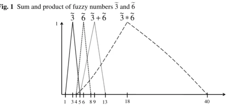
Fig. 1 Sum and product of fuzzy numberse3 ande6

1

3~ 6~

~6 3~

+ 6~

~3

∗

1 3 4 5 6 8 9 13 18 40

Note: is not a triangular fuzzy number.~6 3

~∗

– semistrictly quasi-concave on X if µ

yeis quasi-concave onX and (4) holds for everyx,y∈Xand everyλ∈(0,1)withλx+ (1−λ)y∈X,µ_ye(λx+ (1−λ)y)∈ (0,1)andµ

ey(x)6=µ

ey(y).

Fuzzy arithmetic operations are defined by Dubois and Prade [18] based on the extension principle proposed by Zadeh [89, 90, 91]:

Definition 6 (Fuzzy arithmetic)Letaeandebbe two fuzzy numbers with member- ship functions µ

aeand µ

eb. The membership function µ

ec of the fuzzy number that results from the operationec=ea◦eb,◦ ∈ {+,−,∗, /}, is defined as

µec(z) = sup

x◦y=z

min{µ

ea(x),µ

eb(y)}.

An equivalent definition draws onα-cuts and interval arithmetic [35, chapter 4].

Figure 1 demonstrates arithmetic on triangular fuzzy numbers in a sample case.

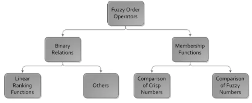
While there is a consensus in the literature on how to perform arithmetic oper- ations on fuzzy numbers, there is no universally accepted way to order fuzzy num- bers. A key concept of ordering fuzzy numbers is the usage of a ranking function R:F(R)→R, with aeeb if and only if R(a)e ≤R(eb) and ea≈eb if and only if R(a) =e R(eb)(see, for example, [50]).Ris called linear if and only ifR(ae+λeb) = R(a) +e λR(eb),λ ∈R. A second option is to draw on a (lexicographic) ranking func- tionR⁰:F(R)→R×R[28] based on the concepts of possibilistic mean value and variance of a fuzzy number [8]. Third, ranking fuzzy numbers can also draw on in- dices based on possibility theory [21].

While ranking functions support a crisp decision of whether a fuzzy number ea is smaller than or equal to a fuzzy numbereb, a different approach based on fuzzy relations assigns a value with whichaeis smaller than or equal toeb[61]. The relation onF(R)×F(R)is valued such thatµ:F(R)×F(R)→[0,1].µ(ea,eb)can be regarded as the degree with whichaeis smaller than or equal toeb.

While fuzzy relations, which enable the comparison of fuzzy numbers, are ap- plied to fuzzy subsets ofF(R)×F(R), Zimmermann [95] proposes an extension of comparison operators of crisp numbers in order to compare crisp numbers in a fuzzy

sense. Here, relations are fuzzy subsets ofR×R, i.e. the relationon R×Ris valued such thatµ:R×R→[0,1].

In the literature a fuzzification of the max and min operations has been proposed.

One of the key concepts was proposed by Dubois and Prade [18]:

Definition 7 (Fuzzy max/min)Letaeandebbe two fuzzy numbers with membership functionsµ

aeandµ

eb. The “fuzzy max” ofeaandeb, which we denote byec=max(g a,eeb), has a membership functionµ

ecsuch that µec(z) = max

max{x,y}=zmin{µ

ea(x),µ

eb(y)}.

In the same way,de=gmin(a,eeb)has a membership functionµ

desuch that µde(z) = max

min{x,y}=zmin{µ

ae(x),µ

eb(y)}.

In the next section we present the results of our literature review.

3 Duality in fuzzy linear programming

In order to structure the findings of the literature, FLP models are classified according to the components that can be fuzzified. In a FLP, the maximization of the objective function (max), the order operator of constraints (≤), the limit values of constraints (b), the coefficients of the objective function (c), the coefficients of constraints (A), and the decision variables can be fuzzified. Each of the model components can be either crisp or fuzzy. Because of the limited practical usefulness of fuzzy decision variables (cf. succeeding paragraph) and in order to keep the number of classes man- ageable, we do not explicitly provide a dimension for the type of decision variables.

When decision variables are fuzzy, the optimal solutions of such problems are also fuzzy. However, in most real-world applications decision makers require crisp solutions to make a decision. For example, Nasseri et al. [51] consider a FLP profit maximization problem, where the produced units of products are represented as fuzzy sets. This implies that the optimal number of units to be produced is also a fuzzy num- ber. However, companies can produce only a crisp number of units, which needs to be considered in the setup of production machines. On the other hand, fuzzy solutions can have practical benefits in situations where crisp decisions are not derived directly from fuzzy solutions, but fuzzy solutions represent the input for further optimization problems. For example, fuzzy solutions might be the result of an optimization prob- lem that looks for optimal market prices of a good. These fuzzy prices can then be used as (fuzzy) coefficients in a further optimization problem that looks for (crisp) solutions of a production plan. However, we still admit that the practical applicability of fuzzy solutions is limited. For the sake of completeness of theoretical approaches, we discuss LP models with fuzzy variables in Subsection 3.5.

Overall, our classification results in a number of 2⁵−1=31 potential classes of fuzzy linear programs if we require a model to have at least one fuzzy component. A similar classification is proposed by Baykasoglu and Goecken [2], but the researchers

do not distinguish between fuzzifying the order operator and the limit values of the constraints. However, since a fuzzy order operator can also be used to compare crisp numbers (see section 2.2) and fuzzy numbers can only be compared by a fuzzy order operator, we consider this separation necessary.

Table 1 shows the resulting classes and the references that contribute to the dual- ity theory of the respective class. While columns represent (five) model components, which can be fuzzified, rows correspond to (31) classes of fuzzy linear programs. The symbolXin row no.iand column no. jindicates that classiis fuzzified with regard to model componentj; otherwise the table entry is empty. Table 1 shows that some of the 31 potential classes of fuzzy linear programs are impossible and are thus excluded from further consideration: a) When coefficients in the objective function are fuzzy then the objective value is fuzzy, too, and underlies a fuzzy maximization operator.

Consequently, classes 2–3,6–7,10–11, and 14–15 are excluded. b) Constraint opera- tors (≤) must be fuzzy ifb,A, or both are fuzzy. Thus, classes 1,3,4-7,17, and 19-23 are excluded. To sum up, among the 31 potential classes of fuzzy linear programs only 14 classes remain feasible. We found that among these 14 classes, only seven classes (classes 8,16,18,24,28,30,31) have been addressed in the literature. The last column lists references for each of these classes; blank entries indicate that we have not found any reference for the respective class.

Some of the existing papers work with arbitrary symmetric trapezoidal fuzzy numbers as a definition of the right-hand side of a constraint, which is not in ac- cordance with the idea behind the constraints in FLP. In particular, they allow a fuzzy right-hand side to be modeled as a fuzzy number with a non-zero left/right spread, which implies that there does not exist a level under/over which the left-hand satis- fies the constraint with certainty. This contradicts the interpretation of the constraints of FLP program, where a tolerance level above/below the certainty level is given.

However, since most of the trapezoidal fuzzy numbers discussed in the presented works can be additionally restricted to have a zero left/right spread, we discuss the approaches further under the condition that they are only applicable with this addi- tional restriction. An exception here is Nasseri et al. [51] where the authors require the use of fuzzy numbers with positive left and right spread. As a result, we believe that the paper does not provide a useful contribution to duality in FLP and exclude it from further discussion.

Table 1 shows that with regard to fuzzy models of class 28 we found two papers in the literature. These approaches use fuzzy decision variables in the primal problem and crisp decision variables in the dual problem. However, the authors do not provide a sound justification for simply mapping fuzzy numbers onto crisp numbers. We thus argue that the presented approaches do not provide any additional value to the field of fuzzy duality theory and thus exclude these from further discussions. As a result, the number of considered classes reduces to six.Finally, as discussed in the previous section, we mark those papers which define fuzzy numbers different from Definition 3.

We now present literature results for those feasible classes where we found refer- ences (classes 8,16,18,24,30,31). The order of presentation is in the order of ascend- ing numbers of classes with two exceptions. The first one is due to the fact that many papers draw on the early ideas of Hamacher et al. [26] and R¨odder and Zimmermann

Table 1 Classification of fuzzy linear programs.

Class Objective Constraints Limit values Coefficients of Coefficients of References of constraints objective function constraints

(max) (≤) (b) (c) (A)

(1) X impossible

(2) X impossible

(3) X X impossible

(4) X impossible

(5) X X impossible

(6) X X impossible

(7) X X X impossible

(8) X [77]

(9) X X

(10) X X impossible

(11) X X X impossible

(12) X X

(13) X X X

(14) X X X impossible

(15) X X X X impossible

(16) X [44]

(17) X X impossible

(18) X X [77],[7]⁽⁴⁾

(19) X X X impossible

(20) X X impossible

(21) X X X impossible

(22) X X X impossible

(23) X X X X impossible

(24) X X [3, 63, 26, 93, 25]

(25) X X X

(26) X X X

(27) X X X X

(28) X X X [45, 47](1),(2),(3),(4)

(29) X X X X

(30) X X X X [50](1),(2),(4),[51](1),(2),(3),(4)

(31) X X X X X [87, 31, 61, 60, 62, 25],

[28]⁽¹⁾,[46]^(2),(4)

(1)fuzzy decision variables

(2)duality results are meaningful only when the left (right) spread of trapezoidal fuzzy numbers on right-hand side of≤(≥) constraints equals zero

(3)excluded from further discussion due to theoretical weaknesses

(4)the definition of fuzzy numbers differs from Definition 3

[63], which are used for deriving duality results in class 24. Thus, this class is pre- sented first. The second exception is due to the separate discussion in Subsection 3.5 of approaches, which consider fuzzy decision variables.

In labeling the optimization problems we generally used the following conven- tion: primal problems in subsectioniare labeled(Pi); dual problems in subsectioni are labeled(Di). In case of more than one approach in a given subsection and differ- ence between the primal or dual problems, we use lower case letters to differentiate between the approaches, i.e. the first primal problem in subsectioniis labeled(Pia).

Derived problems are labeled using additional prime marks. Important auxiliary prob-

lems are labeled(Ai), whereiis initialized at one and increased with the number of labeled problems.

In the following subsections, we present the duality results of the literature re- garding the various classes of fuzzy linear problems with a particular focus on du- ality theorems as they are known from duality theory of crisp linear programming.

We want to note that (1) while we checked the literature for included proofs of dual- ity theorems, we did not investigate whether further duality theorems can be derived from the findings of the respective researchers as we believe that such an investigation is beyond the scope of a literature review, and (2) some of the papers draw on formu- lations of “strong duality” and “complementary slackness” that are slightly different from the common definitions presented in Subsection 2.1.

3.1 Class 24: Fuzzy maximization and fuzzy constraints The primal optimization problem of this class looks as follows:

max]_xc^tx s.t. Axb

x≥0

(P1) In this case, there is only uncertainty regarding the maximization and comparison operators so “max” and “” need to be specified. We found four papers [63, 3, 25,g 26] which deal with(P1)as its primal problem and present them in the following subsections. At the end of this section we provide a brief overview of the discussed approaches.

3.1.1 Approach of R¨odder and Zimmermann (1980)

The paper by R¨odder and Zimmermann [63] does not directly consider problem(P1) as its primal problem. However, as it deals with uncertainty regarding the optimal value of the objective as well as the degree of satisfaction of the constraints of the crisp equivalent of(P1), we present it here. R¨odder and Zimmermann [63] define their approach based on the idea that the solution of(P1)in the crisp case is the one that maximizes the Lagrangian function:

L(x,y) = c^tx

|{z}

primary

+y^t(b−Ax)

| {z }

secondary

. (4)

The researchers interpretL(x,y)as the total profit for a producer (primary plus sec- ondary), who producesx, whereyrepresents the price of production resources on the market,ccontains the prices for the production on the market,Ais the technology matrix andbare the available resource capacities of the producer.

In a fuzzy setting the producer does not maximize his profit, but rather has a certain aspiration levelc^tx⁰for the primary profit that s/he aims to reach, i.e. the maximiza- tion operator in the primal problem is fuzzy. Moreover, the producer is said to have a degree of satisfaction from his secondary profity^t(b−Ax)as a function of the prices

on the markety. Let the membership functions of the primary and the secondary profit beµ(c^tx,c^tx⁰)andµ(Ax,b,y), respectively. To solve(P1), the researchers follow the symmetrical approach of [4] so that in such an optimization problem the objective is treated as a constraint and the solution is the one that maximizes the intersection of the membership functions of the objective and the constraints. Thus, the solution of(P1)is, for given price of the resources on the markety, the one that satisfies

x=argmaxx≥0(min{µ(c^tx,c^tx⁰),µ(Ax,b,y)}). (5) The primal problem(P1)can then be rewritten as

maxx,αα

s.t.µ(c^tx,c^tx⁰)≥α µ(Ax,b,y)≥α x≥0

α∈R

(P1a)

Note that the primal problem is defined as a parametric problem for a givenyand its optimal solution is a pair(α(y),x^∗(y)).

The dual problem is defined analogously to the primal problem, however, in this case the decision-maker is not the producer, but the market with an analogous interpre- tation. The membership functions of the objective of the dual problem and the con- straints areµ(b^ty,b^ty⁰)andµ(A^ty,c,x)respectively. The dual problem can then be rewritten as a parametric problem ofxwith an optimal solution(κ(x),y^∗(x)):

min_y,κκ

s.t.−µ(b^ty,b^ty⁰)≤κ

−µ(A^ty,c,x)≤κ y≥0

κ∈R

(D1a)

The researchers define:

X⁰={x≥0|∀y≥0 :y^tb<0⇒y^tAx≤0}

Y⁰={y≥0|∀x≥0 :c^tx>0⇒y^tAx≥0}

as the set of solutions of(P1a)and(D1a)respectively, where the two problems are bounded. To prove duality, the researchers restrict the setsX⁰andY⁰to the setsX andY respectively:

X={x≥0|∀y≥0 :y^tb≤0⇒y^tAx≤0}

Y ={y≥0|∀x≥0 :c^tx≥0⇒y^tAx≥0}

and by applying Farkas’ lemma show that they are equivalent to:

X={x≥0|∃β ∈R,β≥0,βb≥Ax}

Y={y≥0|∃γ∈R,γ≥0,γc^t≤y^tA} (6)

The researchers then restrict the solution set of (P1a)and(D1a)toX andY as follows:

max_x,α,βα s.t.µ(c^tx,c^tx⁰)≥α

µ(Ax,b,y)≥α x≥0

α∈R βb≥Ax γc^t≤y^tA β ≥0 γ≥0

(P1a’)

miny,κ,γκ

s.t.−µ(b^ty,b^ty⁰)≤κ

−µ(A^ty,c,x)≤κ y≥0

κ∈R βb≥Ax γc^t≤y^tA β≥0 γ≥0

(D1a’)

Note that in(P1a⁰)γandyare given as parameters, while in(D1a⁰)βandxare given as parameters.

Weak duality For any two optimal solutions(α(y),x^∗(y),β(y))and(κ(x),y^∗(x),γ(x)) of(P1a⁰)and(D1a⁰)respectively the following holds:

γ

β(y)c^tx^∗(y)≤b^ty ∀y∈Y

c^tx≤_γ(x)^β b^ty^∗(x) ∀x∈X (7) Note that the presented weak duality theorem is a relation of the elements ofXandY and would hold regardless of the formulation of(P1a)and(D1a)and regardless of whetherxandyare optimal.

3.1.2 Approach of Bector and Chandra (2002)

The paper by Bector and Chandra [3] also addresses(P1)as the primal problem and modifies the approach by R¨odder and Zimmermann [63]. To compare crisp numbers in a fuzzy sense, given two real numbersAandB,ABis defined in the paper using a linear, monotone membership functionµ:R×R→[0,1]as follows:

µ(A,B) =







0 A>B+f₀ 1−^A−B_f

0 B<A≤B+f0

1 A≤B

(8)

where f₀>0 is the tolerance interval describing the extent to which the constraint can be violated.µis defined analogously.

Bector and Chandra [3] define “max” following also the approach of Bellman andg Zadeh [4]. The researchers transform the objective into a constraint using the aspira- tion levelc^tx⁰.(P1)can then be rewritten as:

c^txc^tx⁰ Axb x≥0.

(P1b)

The solution of(P1b)is the pair(x,α)such that max_x,αα

s.t.µ(c^tx,c^tx⁰)≥α µ(Ax,b)≥α x≥0

α∈[0,1].

(P1b’)

Note thatµ(Ax,b)is not a single number, but rather a vector containing, for each constrainti, the valueµ(i)(A_ix,b_i), whereµ(i)stands for the corresponding mem- bership function. Let the tolerance interval of the membership functionµ(i) be p_i (see (8)) and p= (p₁, ...,p_m). Let, in addition p₀ be the tolerance interval of the membership functionµ(c^tx,c^tx⁰). The researchers define the dual problem as fol- lows:

ming_yb^ty s.t. A^tyc

y≥0

(9)

After transforming the objective to a constraint with aspiration levelb^ty⁰, this prob- lem becomes

b^tyb^ty⁰ A^tyc y≥0.

(D1b) The crisp linear problem analog to(P1b⁰)is then

miny,κ−κ s.t.µ(b^ty,b^ty⁰)≥κ

µ(A^ty,c)≥κ κ∈[0,1]

y≥0

(D1b’)

with a solution(y,κ).

Note thatµ(A^ty,c)is not a single number, but rather a vector containing, for each constraint j, the value µ(j)((A^t)_jy,c_j), whereµ(j) stands for the corresponding membership function. Let the tolerance interval of the membership functionµ(j)be q_j (see (8)) andq= (q₁, ...,q_n). Let, in additionq₀be the tolerance interval of the membership functionµ(b^ty,b^ty⁰).

Weak duality For each feasible solution(x,α)of(P1b⁰)and each feasible solution (y,κ)of(D1b⁰)the following inequality holds:

(α−1)p^ty−(κ−1)q^tx≤(b^ty−c^tx), (10) The theorem is equivalent to the crisp weak duality theorem in caseα=κ=1.

Bector and Chandra [3] additionally show that, given two feasible solutions(x,α) and(y,κ)of(P1b⁰)and(D1b⁰), respectively, the following implication holds:

If the subsequent conditions hold – (α−1)p^ty+ (κ−1)q^tx= (b^ty−c^tx)

– (α−1)p₀+ (κ−1)q₀= (c^tx−b^ty) + (b^ty⁰−c^tx⁰) – c^tx⁰−b^ty⁰≤0,

then(x,α)and(y,κ)are optimal solutions.

In this subsection, we would also like to mention the paper by Gupta and Mehlawat [25]. It follows an approach that is very similar to that of Bector and Chandra [3] and that differs in the type of the membership functions (exponential membership func- tions) for the constraints and objectives of(P1b)and(D1b). The researchers provide the same duality results with a modification for the particular membership functions.

In addition, Gupta and Mehlawat [25] show how their approach can be applied to problems of class 31 by using ranking functions for the comparison of fuzzy num- bers and transforming the fuzzy problems of class 31 to the problems (P1b⁰) and (D1b⁰). Due to the similarities of the ideas in the papers by Bector and Chandra [3]

and Gupta and Mehlawat [25], we omit a detailed presentation of the results of Gupta and Mehlawat [25].

3.1.3 Approach of Hamacher et al. (1978)

The paper by Hamacher et al. [26] considers a primal problem with fuzzy maximiza- tion and a mixture of fuzzy and crisp constraints. Since crisp contraints can be seen as a special case of fuzzy constraints, we consider the paper in this class. The primal problem is defined as follows:

max]_xc^tx s.t. Axb

Dx≤f x≥0

(P1c)

Similar to the other two approaches presented in this section,max is defined by theg membership function µ(c^tx,c^tx⁰), wherec^tx⁰ is the aspiration level of the deci- sion maker. is defined by the membership function µ(Ax,b)representing soft constraints. Following the symmetrical approach of Bellman and Zadeh [4] and the assumption of linear membership functions, the researchers rewrite(P1c)as the fol-

lowing crisp linear optimization problem:

max_x,αα

s.t.µ(c^tx,c^tx⁰)≥α µ(Ax,b)≥α Dx≤f x≥0

µ(c^tx,c^tx⁰)∈[0,1]

µ(Ax,b)∈[0,1]

(P1c’)

The dual problem is defined as the crisp dual of(P1c⁰), which is also a crisp linear problem and strongly depends on the membership functions chosen. The researchers provide an economic interpretation of the variables of the dual problem and admit that as opposed to the crisp case not all of them can be interpreted as shadow prices. Thus, they perform sensitivity analysis on the primal problem to“... derive the functional relationships between changes of components of the right-hand-side and changes of the optimal value of the primal objective functions ...”(p. 270). The researchers do not prove any duality results.

3.1.4 Summary

To sum up, the paper by R¨odder and Zimmermann [63] aims to define fuzzy dual- ity in a very intuitive way, using a clear economic interpretation. However, the ap- proach suffers from some disadvantages, such as the particular form of the member- ship functions, which allow values higher than one and lower than zero. In addition, the researchers show only weak duality, which they prove in a mathematically very restricted setting.

The paper by Bector and Chandra [3] modifies the ideas in R¨odder and Zimmer- mann [63] to address most of the above mentioned disadvantages. In addition, here the optimization problems are easier to solve than in [63]. However, there are also a few disadvantages. First, the approach is restricted to the use of linear monotone membership functions. Secondly, they prove only weak duality and provide a cri- terion to test solutions for optimality. However, Bector and Chandra [3] admit that strong duality would generally not hold.

Finally, the paper by Hamacher et al. [26] extends the literature on duality theory in fuzzy linear optimization by performing sensitivity analysis on the primal problem.

3.2 Class 8: Fuzzy constraints

The primal optimization problem in this class is max_xc^tx s.t. Axb

x≥0.

(P2)

Note that here only the fuzzy order operator must be defined. We found only one paper [77] that addresses duality of this problem type. The researcher definessimi- larly to Bector and Chandra [3] through the use of a continuous and strictly monotone membership functionµ. An example of such a function is shown in(8).

The difference to problems of class 24 (fuzzy maximization and fuzzy constraints) is that here the symmetric principle of Bellman and Zadeh [4] cannot be applied as max is a crisp operator and not a fuzzy one and thus the objective and the constraints cannot be treated symmetrically. Therefore, Verdegay [77] suggests a parametric ap- proach where the degree to which the constraints of(P2)are satisfied is represented by an exogenously given parameterα.(P2)can then be transformed into:

max_x c^tx

s.t. µ(Ax,b)≥α α∈[0,1]

x≥0.

(P2’)

This results in a fuzzy set as an optimal value because, for each degree of certainty α, we obtain a different solutionx.

The dual problem in reference [77] is defined as ming_yeb^ty s.t. A^ty≥c

y≥0,

(D2) which has the same fuzzy components as the problems of class 18. (D2)is trans- formed into a parametric problem with an exogeneously given parameterβ as fol- lows:

min_yb^ty

s.t. µ_j(b_j)≥1−β,j∈1, ..,m A^ty≥c

y≥0 β∈[0,1].

(D2’)

where,µ_jare membership functions for the coefficients of the objective. However, it is not clear from the paper why the equivalence between(D2)and(D2⁰)holds. The interested reader should turn to [24, pp. 231ff] for more information. For continuous and strictly monotone membership functions,(D2⁰)can be transformed to

min_y∑_jµ⁻¹_j (1−β)y_j s.t. A^ty≥c

y≥0 β∈[0,1].

(11)

Here, in contrast to(P2⁰), the parameterβ does not affect the feasible region, but only the value of the objective function.

Strong duality GivenP2⁰(resp.D2⁰) with continuous and strictly monotone mem- bership functionsµ(resp.µj∀j) and the corresponding dual problem problem D2⁰(resp.P2⁰), the optimal objective values are the same fuzzy sets. The proof is based on crisp duality theory.

An advantage of this approach is that it applies very elegantly the main reason for the popularity of duality theory, namely that by solving one of the primal or dual problems we can find the solution of the other. In this case, the primal problem is very difficult to solve as it contains the parameterαin each of its constraints, i.e. the parameterα determines the feasible region. The problem(D2)on the other hand can be transformed into a crisp linear problem, where the parameterβ is only part of the objective function. This makes(D2)much easier to solve. Note that the paper can just as well be classified in class 18 since all the results hold also when the primal problem is(D2). Then the dual problem would be(P2).

3.3 Class 18: Fuzzy maximization, fuzzy coefficients of objective function The primal problem in this section is

max]_xec^tx s.t. Ax≤b

x≥0.

(P3)

We found only one paper that deals with this type of primal problem [7]. The re- searchers work with general fuzzy numbers. Note that this problem is equivalent (in terms of parts that are fuzzified) to the problem(D2)presented in subsection 3.2.

Cadenas Figueredo and Jim´enez Barrionuevo [7] follow the approach in Subsection 3.2 and rewrite(P3)as a parametric problem with an exogeneously given parameter α:

max_x c^tx

s.t. µ_j(c_j)≥α,j∈1, ...,n Ax≤b

x≥0 α∈[0,1],

(P3’)

where the membership functionµ_j(c_j)is non-negative on the interval[c_j−d¹_j,c_j+ d²_j]∀jand equals to one in the interval[c_j,c_j]. Problem(P3⁰)is then equivalent to the following interval parameter linear programming problem:

maxx [c−d¹α,c+d²α]x s.t. Ax≤b

x≥0 α∈[0,1],

(P3”)

wherec= (c₁, ...,c_n),c= (c₁, ...,c_n),d¹= (d₁¹, ...,d_n¹),d²= (d₁², ...,d_n²).

In the next step the researchers derive the crisp dual problem of(P3⁰⁰)as follows:

min_yb^ty

s.t. A^ty≥[c−d¹α,c+d²α] y≥0

α∈[0,1]

(12)

Let

Kmin={y≥0|A^ty≥c−d¹α}

K={y≥0|A^ty≥c^∗,c^∗∈[c−d¹α,c+d²α]}

K_max={y≥0|A^ty≥c+d²α}

ThenK_max⊂K⊂K_min. The researchers use these relationships to show that the op- timal value of problem(12)is bounded from above and below by the optimal values of the following two auxiliary crisp linear parametric problems:

min_yb^ty

s.t. A^ty≥c−d¹α y≥0

α∈[0,1]

(A1)

min_yb^ty

s.t. A^ty≥c+d²α y≥0

α∈[0,1]

(A2)

Based on the duality between(P3⁰⁰)and(12), the researchers show that, ify_min(α) is the optimal solution of(A1)andy_max(α)the optimal solution of(A2), then the optimal value of the objective function of(P3⁰⁰)for a givenα∈[0,1]is included in the interval:

[b^ty_min(α),b^ty_max(α)]

The dual problem in this subsection is defined as:

min_yb^ty s.t. A^tyc

y≥0.

(D3) Note that by choosing suitable membership functions, both(A1)and(A2)can be rewritten in the form of (D3). Thus, it can be shown that the optimal value of the objective function of(P3)is bounded by the optimal values of the objective functions of two fuzzy linear optimization problems of type(D3). Similarly, the researchers prove that the optimal value of the objective function of an optimization problem of type(D3)is bounded by the optimal value of the objective functions of two fuzzy optimization problems of type(P3).

Strong duality Given a problem(P3), there always exist two problems of type(D3) so that the optimal value of the objective function of(P3)is both lower and upper bounded by the optimal values of the objective functions of the problems of type (D3). Analogously, given a problem of type(D3), there always exist two prob- lems of type(P3)so that the the optimal value of the objective function of(D3) is both lower and upper bounded by the optimal values of the objective functions of the problems of type(P3).

To sum up, the paper by Cadenas Figueredo and Jim´enez Barrionuevo [7] uses linear interval programming to define the concept of duality. The approach is very intuitive and quite innovative. Moreover, the results in this paper extend and systematize the work of Verdegay [77]. However, the researchers do not present any other duality theorems except strong duality.

3.4 Class 31: Fuzzy maximization, fuzzy constraints, fuzzy coefficients of constraints, fuzzy limit values of constraints and fuzzy coefficients of objective function

The primal fuzzy linear optimization problem in this class is defined as follows:

max]_xec^tx s.t. Axe eb

x≥0

(P4)

In order to properly define problem (P4), we need to define which fuzzy numbers are used and how the operators “” and “max” are specified. The literature [60,g 31, 61, 87, 46, 62] is not homogeneous in this regard, which results in syntactically similar, but semantically different duality theorems. Thus, for each of the papers we explicitly present the respective results of the researchers and finally provide a brief overview of the approaches at the end of this subsection.

3.4.1 Approach of Inuiguchi et al. (2003)

The works by Ram´ık [60] and Inuiguchi et al. [31] follow a very similar approach, therefore we discuss only the second one here. Inuiguchi et al. [31] use compact, strictly convex, normal fuzzy subsets of the real numbers. They defineas a fuzzy relation with a membership functionµ:F(R)×F(R)→[0,1], which is based on t-norms, t-conorms and valued relations. Inuiguchi et al. [31] define max using ang exogenously given aspiration levelde∈F(R)and the fuzzy relation, in which their approach differs from the approaches in the other papers presented in this subsection.

The researchers rewrite(P4)as follows:

ec^txde Axe eb x≥0

(P4a)

Inuiguchi et al. [31] define the set ofα-feasible solutions⁶, 0≤α≤1, as thosex≥0 which satisfy the constraints of(P4)(i.e.Axe eb,x≥0 in(P4a)) at least with degree α. Anα-satisficing solution is anα-feasible solutionxthat additionally satisfies the objective of(P4)(i.e. the constraintec^txdein(P4a)) at least with degreeα. This concept is based on the symmetric approach of Bellman and Zadeh [4].

The dual problem in [31] is defined as follows:

eb^tyeh Ae^tyec y≥0

(D4a)

6 Note that we define the concepts ofα-feasible andα-satisficing solution here for the particular case to which the researchers apply duality theory. Their definition is much broader.

Weak duality Under some assumptions (p. 171), for eachα-feasible solutionxof (P4a)and eachα-feasible solutionyof(D4a)the following inequality holds:

∑

ce_j^R(1−α)x_j≤

∑

i

be_i^R(1−α)y_iforα∈[0.5,1) (13) They call property (13) “a weak form of the duality theory”. Here,ce_j^R(1−α)and be_i^R(1−α)are the upper bounds of the “(1−α)−cuts” ofce_jandbe_i, respectively, i.e.ce_j^R(1−α) =supce_j[1−α]andbe_i^R(1−α) =supbe_i[1−α].

Strong duality If there exists an α-satisficing solution for (P4a) and a (1−α)- satisficing solution for(D4a), then and under some additional assumptions (p.

172) there exist anα-satisficing solutionx^∗for(P4a)and a(1−α)-satisficing solutiony^∗for(D4a)such that

∑

cejR(α)x_j=

∑

i

bei

R(α)y_i. (14)

3.4.2 Approach of Ram´ık (2005)

The approach of Ram´ık [61] modifies the approach of Inuiguchi et al. [31]⁷. More- over, the ideas of Ram´ık [62] can be seen as an extension of the ideas of Ram´ık [61].

While Ram´ık [61] proves duality results only for the case, where the comparison op- erators in the primal problem are based on t-norms and those in the dual are based on t-conorms, Ram´ık [62] proves also weak and strong duality for the opposite case. We thus believe that presenting the ideas of Ram´ık [61] in detail is enough to understand both papers.

Ram´ık [61] similarly to Inuiguchi et al. [31] definesas a fuzzy relation, which is based on t-norms, t-conorms and valued relations. In contrast to Inuiguchi et al. [31], in order to determinemax, [61] does not transform the objective into a constraint.g Instead he uses the following relation on the set of fuzzy numbers, which is a binary relation for a givenα∈(0,1]and fuzzy numbersaeandeb:

ae≺_αeb⇔

µ(ea,eb)≥α∧µ(eb,ea)<α

(15) An α-efficient solution for (P4) (i.e. definition of max) is then defined as ang α- feasible solutionxsuch that there does not exist anα-feasible solutionx⁰withce^tx≺_α ec^tx⁰.

Ram´ık [61] defines the dual problem as follows:

ming_yeb^ty s.t. Ae^tyec

y≥0

(D4b) where the comparison operatoris the dual operator ofRam´ık [61, p. 26f.], as used in the primal problem (P4).

7 The researcher, too, works with the same type of fuzzy numbers as Inuiguchi et al. [31] with the difference that the membership functions of Ram´ık [61] are semistrictly quasi-concave.

Weak duality Ram´ık [61] defines two weak duality theorems. The first one states that under some assumptions (p. 33f) for anα-feasible solutionxof(P4)and a (1−α)-feasible solutionyof(D4b)the following inequality holds:

∑

ce_j^R(α)x_j≤

∑

i

be_i^R(α)y_i (16)

wherece_j^R(α)andbe_i^R(α)are defined as in subsection 3.4.1.

Regarding the second weak duality theorem, the researcher proves that if

∑

ce_j^R(α)x_j=

∑

i

be_i^R(α)y_i

thenxisα-efficient for(P4)andyis(1−α)-efficient for (D4b). This theorem can be used as a test criterion for optimality.

Strong duality Under some assumptions (p. 35) (P4) has anα-efficient solutionx^∗ and(D4b)has a(1−α)-efficient solutiony^∗and the following equation holds:

∑

j

ce_j^R(α)x_j=

∑

i

be_i^R(α)y_i (17)

3.4.3 Approach of Wu (2003)

The researcher [87] works with normal, convex fuzzy subsets of the real numbers with upper-semicontinuous membership functions and compactα-cut forα =0. He definesfor two fuzzy numberseaandebas follows:

aeeb:⇔

ea(α)^L≥eb(α)^L∧a(α)e ^R≥eb(α)^R∀α∈[0,1]

(18) Hereea(α)^Lis the lower bound of the “α−cut” ofa. Note thate is a binary relation on the set of fuzzy numbers, as it is not parametrized byα.

In contrast to the approaches of Inuiguchi et al. [31] and Ram´ık [61], this paper defines the primal problem as a minimization problem and the dual problem as a maximization problem:

ming_xce^tx s.t. Axe eb

x≥0

(P4c)

max]_yeb^ty s.t. Ae^tyce

y≥0

(D4c) The researchers define the optimal solution of(P4c)as the feasible solutionx^∗that minimizesce^txover all feasible solutions according to the definition of. The optimal solution of(D4c)is defined analogously.