Computational and Cognitive Neuroscience
D I S S E R T A T I O N
zur Erlangung des akademischen Grades Doctor rerum naturalium
(Dr. Rer. Nat.) im Fach Physik
Spezialisierung: Theoretische Physik eingereicht an der
Mathematisch-Naturwissenschaftlichen Fakultät Humboldt-Universität zu Berlin
von
M. Sc. Sebastian Vellmer
Präsidentin der Humboldt-Universität zu Berlin:
Prof. Dr.-Ing. Dr. Sabine Kunst
Dekan der Mathematisch-Naturwissenschaftlichen Fakultät:
Prof. Dr. Elmar Kulke Gutachter:
1. Prof. Dr. Benjamin Lindner (HU Berlin) 2. Prof. Dr. Igor M. Sokolov (HU Berlin)
3. Prof. Dr. Magnus J.E. Richardson (University of Warwick)
Tag der mündlichen Prüfung: 02. Juli 2020
This thesis is concerned with the calculation of statistics, in particular the power spectra, of point processes generated by stochastic multidimensional integrate-and-fire (IF) neurons, networks of IF neurons and decision-making models from the corresponding Fokker-Planck equations.
In the brain, information is encoded by sequences of action potentials, the spike trains that are emitted by its most important elements, the neurons. In studies that focus on spike timing and not on the detailed shape of action potentials, IF neurons that drastically simplify the spike gen- eration have become the standard model since they are easy to use and even provide analytical insights. Stochastic IF neurons are particularly advantageous when studying the influence of noise on the firing variability and information transmission. One-dimensional IF neurons do not suffice to accurately model neural dynamics in many situations. However, the extension towards multiple dimensions yields realistic subthreshold and spiking behavior at the price of growing complexity.
The first part of this work develops a theory of spike-train power spectra for stochastic, multidi- mensional IF neurons. From the corresponding Fokker-Planck equation, a set of partial differential equations is derived that describes the stationary probability density, the firing rate and the spike- train power spectrum. The equations are solved numerically by a finite-difference method for three special cases. The effect of temporally correlated input fluctuations, so-called colored noise, is stud- ied by means of a one-dimensional Markovian embedding that generates either high-pass-filtered (cyan or white-minus-red) or low-pass-filtered (white-plus-red) noise as input for a leaky IF (LIF) neuron. The theory is also applied to white-noise-driven exponential IF neurons with adaptation and, as a three-dimensional example, to a LIF neuron driven by narrow-band noise. Many exam- ples of solutions are presented and compared to simulations in order to test the theory, to display the variety of spectra and to gain a better understanding of the influence of neural features on the spike-train statistics. Furthermore, a set of equations is derived and tested to calculate the Padé approximation of the spectrum at zero frequency yielding an analytical function that is accurate at low frequencies and also matches the high-frequency limit.
In the second part of this work, a mean-field theory of large and sparsely connected homogeneous networks of LIF neurons is developed that takes into account the self-consistent temporal correla- tions of spike trains. Neural input, as the sum of many independent spike trains, is approximated by colored Gaussian noise that is generated by a multidimensional Ornstein-Uhlenbeck process (OUP) yielding a multidimensional IF neuron. In contrast to the first part, the coefficients of the OUP are initially unknown but determined by the self-consistency condition and define the solution of the theory. Since finite-dimensional OUPs cannot exhibit arbitrary power spectra, approximations are introduced and solved up to two-dimensional OUPs for one network. An alternative approach is used to explore heterogeneous networks in which the distribution of power spectra is self consistent.
An iterative scheme, initially introduced for homogeneous networks, is extended to determine the distribution of spectra for networks with only distributed numbers of presynaptic neurons and, additionally, distributed synaptic weights.
In the third part, the theoretical framework of the Fokker-Planck equation is applied to the prob- lem of binary decisions from diffusion-decision models (DDM). The theory considers the temporal statistics of decisions in situations in which a subject performs consecutive trials of a decision- making experiment. The decision trains are introduced in which spikes at the decision times capture the experimental results and encode correct and incorrect decisions by their signs. For the analytically tractable DDM, a Wiener process within two boundaries, the statistics of the deci- sion trains including the decision rates, the distributions of inter-decision intervals and the power spectra are calculated from the corresponding Fokker-Planck equation. Nonlinear DDMs arise as the approximation of decision-making processes implemented in competing populations of spiking neurons. For these models, the threshold-integration method, an efficient numerical procedure that was originally introduced for IF neurons, is generalized to solve the corresponding Fokker-Planck equations and determine the decision-train statistics and the linear response of the decision rates.
In dieser Arbeit werden mithilfe der Fokker-Planck-Gleichung die Statistiken, vor allem die Leis- tungsspektren, von Punktprozessen berechnet, die von mehrdimensionalen Integratorneuronen [Engl.
integrate-and-fire (IF) neuron], Netzwerken von IF Neuronen und Entscheidungsfindungsmodellen erzeugt werden.
Im Gehirn werden Informationen durch Pulszüge von Aktionspotentialen kodiert, die von den wichtigsten Komponenten, den Neuronen, ausgesandt werden. In Fällen, in denen das Hauptau- genmerk auf neuronale Pulszeiten gerichtet ist und die genaue Form der Aktionspotentiale eine untergeordnete Rolle spielt, haben sich IF Neurone als Standardmodelle etabliert, in denen der Mechanismus der zur Erzeugung von Aktionspotentialen dient, radikal vereinfacht wird. Die Mo- delle sind leicht anzuwenden und ermöglichen sogar analytische Lösungen, wodurch insbesondere ihre stochastischen Versionen geeignet sind, um den Einfluss neuralen Rauschens auf die Varia- bilität der Pulszeiten und auf die Transmission von Information zu untersuchen. Allerdings sind eindimensionale IF Modelle in vielen Situationen zu einfach und können beobachtetes Pulsverhal- ten nicht beschreiben. Abhilfe kann durch die Erweiterung hinzu mehrdimensionalen IF Neuro- nen geschafft werden, die realistische Modelle bezüglich der unterschwelligen Spannungsdynamik und auch des Pulsverhaltens hervorbringen kann. Im ersten Teil dieser Arbeit wird eine Theorie zur Berechnung der Pulszugleistungsspektren von stochastischen, multidimensionalen IF Neuronen entwickelt. Ausgehend von der zugehörigen Fokker-Planck-Gleichung wird hierzu ein System von partiellen Differentialgleichung abgeleitet, deren Lösung sowohl die stationäre Wahrscheinlichkeits- verteilung und Feuerrate, als auch das Pulszugleistungsspektrum beschreibt. Da keine analytische Lösung bekannt ist, werden die Lösungen für drei spezielle Neuronmodelle numerisch mit einer finite-Differenzen-Methode bestimmt. Mithilfe einer eindimensionalen Markovschen Einbettung, die entweder hochpassgefiltertes (zyanes oder weiß-minus-rotes) oder tiefpassgefiltertes (weiß-plus- rotes) Rauschen generiert, wird der Effekt von Eingangströmen mit zeitlich korrelierten Fluktua- tionen, auch als farbiges Rauschen bekannt, auf das Pulsverhalten eines leaky IF (LIF) Neurons untersucht. Die Theorie wird auch auf ein exponentielles IF Neuron mit Adaptationsstrom, das von weißem Rauschen getrieben wird, und, als ein dreidimensionales Beispiel, auf ein LIF Neuron, das von Schmalbandrauschen getrieben wird, angewandt. Viele Beispiele von Lösungen werden gezeigt und mit direkten numerischen Simulationen verglichen, einerseits um die Theorie zu testen, ande- rerseits um die Vielfältigkeit der Spektren aufzuzeigen und ein Verständnis zu entwickeln, wie sich neuronale Eigenschaften auf die Pulszugstatistiken auswirken. Zuletzt werden Gleichungen herge- leitet und getestet, mit denen eine Padé Approximation berechnet werden kann. Das Resultat der Annäherung ist eine analytische Funktion, die das Leistungsspektrum bei niedrigen Frequenzen präzise beschreibt und auch im Hochfrequenzlimit exakt ist.
Im zweiten Kapitel wird eine Molekularfeldtheorie für große, spärlich verbundene und homogene Netzwerke aus LIF Neuronen entwickelt, in der berücksichtigt wird, dass die zeitlichen Korrela- tionen von Pulszügen selbstkonsistent sind. Neuronale Eingangströme, die sich aus der Summe vieler unabhängiger Pulszüge ergeben, werden durch farbiges Gaußsches Rauschen modelliert, das von einem mehrdimensionalen Ornstein-Uhlenbeck Prozess (OUP) erzeugt wird, sodass sich ein mehrdimensionales IF Neuron ergibt. Die Koeffizienten des OUP sind vorerst unbekannt und sind als Lösung der Theorie über die Selbstkonsistenz der Leistungsspektren des Eingangsstroms und des Pulszuges definiert. Allerdings kann durch endlichdimensionale OUPs kein Rauschen mit be- liebigem Leistungsspektrum erzeugt werden. Daher werden Annäherungen zu der Theorie mit end- lichdimensionalen OUPs eingeführt und für ein Beispielnetzwerk mit ein- und zweidimensionalen OUPs gelöst. Um heterogene Netzwerke zu untersuchen, in denen die Verteilung von Pulszugleis- tungsspektren selbstkonsistent ist, wird ein anderer Ansatz gewählt. Eine iterative Methode, die ursprünglich für homogene Netzwerke eingeführt wurde, wird erweitert um die selbstkonsistente Verteilung zu ermitteln. Zwei Beispielnetzwerke, die einerseits mit einer verteilten Anzahl von prä- synaptischen Verbindungen und, im zweiten Fall, mit zusätzlich verteilten synaptischen Gewischten
scheidungsmodellen [Engl. diffusion-decision models (DDM)] angewendet. Die Theorie ist für Si- tuationen entworfen, in denen ein Subject in einem Experiment sequentielle Entscheidungen in auf- einander folgenden Durchläufen fällt. Zur Beschreibung der experimentellen Resultate werden die Entscheidungszüge eingeführt, in denen Pulse zu den Entscheidungszeiten korrekte und inkorrekte Entscheidungen mit ihrem Vorzeichen kodieren. Explizite Gleichungen für die Entscheidungszug- statistiken, genauer die Entscheidungsraten, Intervallverteilungen zwischen Entscheidungen und Leistungsspektren, werden für den einfachsten und analytisch lösbaren Fall von DDMs, einem Wiener Prozess innerhalb zweier Grenzen, von der Fokker-Planck-Gleichung hergeleitet. Aus der Implementierung von Entscheidungsprozessen in neuronalen Netzwerken gehen nichtlineare DDMs hervor. Für diese Modelle wird die Schwellwertintegrationsmethode [Engl. threshold-integration method] erweitert, die ursprünglich zur Bestimmung der Pulszugstatistiken von nichtlinearen IF Neuronen eingeführt wurde. Diese Methode wird auf Modelle mit zwei Schwellen verallgemeinert, um effizient Lösungen der Fokker-Planck-Gleichung zu bestimmen und damit die Statistiken von Entscheidungszügen und die Suszeptibilitäten der Entscheidungsraten zu berechnen.
Mathematical notation Meaning
δ(x) Dirac delta function
δi,j Kronecker symbol
δ¯i,j = 1−δi,j ’Anti’-Kronecker symbol
hxi ensemble average
ξ(t) Gaussian white noise of unit intensity
∂xf(x) derivative off(x) with respect tox
f(x)
x=a=f(a) value of f ata
f˜(ω) =
∞
R
0
dt eiωtf(t) Fourier transformed over positive half space (f ∗g)(t) =
∞
R
0
dt0f(t0)g(t−t0) convolution off and g
exp(x) exponential function
sinh[x] = [exp(x)−exp(−x)]/2 hyperbolic sine
Θ(x) Heaviside function
Re(x) real part of the complex argument
Da(x) parabolic cylinder function
erf(x) = √2π
x
R
0
du e−u2 error function
arg minxf(x) argument that minimizesf(x)
x mod y modulo operation
A matrix
A−1 inverse matrix
A| transposed matrix
det(A) determinant of matrixA
adj(A) adjoint matrix ofA
Abstract i
Zusammenfassung ii
List of symbols iv
1. Introduction 1
1.1. Fundamentals of probability theory and stochastic processes . . . 3
1.2. Physiological basics of neural networks . . . 6
1.3. Models of stochastic spiking neurons . . . 9
2. Theory of spike-train power spectra for stochastic multidimensional integrate- and-fire neurons 13 2.1. The generalized two-dimensional integrate-and-fire neuron . . . 16
2.1.1. Spike-train statistics of first and second order . . . 17
2.1.2. Fokker-Planck equation and spike-train power spectrum . . . 18
2.1.3. Leaky integrate-and-fire neuron driven by cyan and white-plus-red noise 26 2.1.4. Stochastic exponential integrate-and-fire neuron with adaptation . . . 33
2.2. Generalization to d-dimensional models . . . 39
2.2.1. Harmonic noise driven LIF neuron . . . 41
2.3. Derivatives of the power spectrum and Padé approximation . . . 43
2.4. Summary and discussion . . . 47
3. Mean-field theory of large and sparse recurrent networks including self-consistent temporal correlations of spike trains 49 3.1. Homogeneous network . . . 52
3.1.1. Network dynamics and topology . . . 52
3.1.2. Mean-field conditions and approximations . . . 53
3.1.3. Multidimensional Ornstein-Uhlenbeck process as general source of col- ored Gaussian noise may model neural input . . . 57
3.1.4. Mean-field theory . . . 60
3.1.5. Approximative solutions with finite-dimensional input processes . . . . 62
3.2. Iterative scheme for heterogeneous networks . . . 68
3.3. Summary and discussion . . . 74
4. Statistics of binary-decision sequences 77
4.1. Decision-train statistics for renewal processes . . . 80
4.2. Diffusion-decision model and decision-train statistics . . . 83
4.3. Threshold-integration method . . . 89
4.3.1. Stationary solution . . . 89
4.3.2. Time-dependent solutions: reaction-time densities, interdecision- inter- val distributions and decision-train power spectra . . . 91
4.3.3. Linear response to modulation of input . . . 97
4.4. Summary and discussion . . . 100
5. Summary and conclusion 103 A. Spike-train power spectra of multidimensional integrate-and-fire neurons 105 A.1. Additional condition for Fourier transformed probability density ˜Q forω→0 and ω = 0 . . . 105
A.2. Numerical solution for two-dimensional IF neurons . . . 107
A.2.1. Discretization and boundary conditions . . . 108
A.2.2. Subthreshold dynamics . . . 108
A.2.3. Fire-and-reset operation . . . 109
A.2.4. Stationary density and firing rate . . . 112
A.2.5. Solution in Fourier domain and spike-train power spectrum . . . 113
A.2.6. Convergence and accuracy of the numerical solution . . . 114
A.3. Power spectrum of white-noise-driven LIF neuron . . . 115
A.4. Numerical solution for three-dimensional IF neurons . . . 115
A.5. Derivatives of the spike-train power spectrum at ω= 0 . . . 119
B. Mean-field theory that considers temporal correlations of spike trains 121 B.1. Two-dimensional Ornstein-Uhlenbeck process . . . 121
B.2. Probability transition due to refractory period ford >1 . . . 124
C. Parameters 127 C.1. Theory of spike-train power spectra . . . 127
C.2. Mean-field theory . . . 129
C.3. Diffusion-decision model . . . 130
Bibliography 131
Created by billions of years of evolution, the human brain is a sophisticated machine equipped with the desire and possibly even the capacity to comprehend its own mechanisms. Compared to other measurement difficulties overcome by modern physics, the spatial and temporal scales at which processes happen in the brain can be captured relatively easily (Kandel et al., 2000). The challenging problems arise when one attempts to reverse engineer the brain due to its complexity at different length scales, the lack of symmetry, the uncertainty around which dynamical details are vital for specific tasks and the fact that sensitive living tissue is examined. While microscopic ion channels and single synapses may be studied by the detailed dynamics of the underlying ions and molecules, single nerve cells, neural networks and macroscopic brain regions are much to complex and have to be described by abstract mathematical models that are accompanied by a certain degree of simplification (Koch, 1999;
Dayan and Abbott, 2001; Gerstner et al., 2014). When linking the dynamics of the brain at different scales with macroscopic behavior, it is impossible to establisha priori which details are essential and which might be neglected in a simplified model in order to capture a certain function. For a comprehensive description of the brain, various models must be adapted to fit specific problems and then be assembled like puzzle pieces into a bigger picture. Hence, it is a crucial task for scientists working in the fields of computational neuroscience and neurophysics to create models that reproduce and predict experimental findings and then study them by developing and applying mathematical methods.
It is widely accepted that information in the brain is encoded by sequences of electric pulses, the spike trains, that are emitted by the neurons. Attempts to decipher these neural codes by using approaches from information theory are work in progress and remain a challenging task. Since in vivo neurons are subject to many sources of noise [see for instance Holden (1976); Tuckwell (1989)], the timing of single spikes is unreliable and its relevance regarding information transmission and processing can be questioned. For the description of neural systems, stochastic models are required that can be studied by methods of statistical physics in order to understand, for example, how fluctuations influence the statistics of neural spike trains. An appropriate approach to gain insights in the dynamics of stochastic systems is given by the application of the Fokker-Planck equation, i.e. a partial differential equation describing the temporal evolution of the probability density (Risken, 1984). By the determination of the solution of the Fokker-Planck equation corresponding to stochastic neuron models, analytical formulas have been derived for the spike-train statistics [see for instance Ricciardi (1977);
Brunel and Sergi (1998); Schwalger et al. (2015)] and the dynamics of spiking neural networks
have been investigated by mean-field approaches [see for instance (Brunel, 2000)]. Recorded neural spike-trains are characterized by non-trivial temporal statistics that depend on the single-neuron properties, on the dynamics of the surrounding network that generates neural input, and on the connection between them. Experimentally measured correlations might be useful to gain insights in the underlying mechanisms of a neural network. Furthermore, it cannot be excluded that the temporal correlations of spike trains serve a purpose regarding the computations in the brain, hence, they are worth to be studied in detail. In this work, equations are derived that determine the temporal correlations represented by the spike-train power spectra of stochastic neuron models and networks of spiking neurons by the application of the Fokker-Planck equation.
Linking the dynamics of neural populations to the solution of cognitive tasks is a crucial goal of neuroscience. For perceptual decision making, being one example of a cognitive task, the underlying mechanisms might be implemented by the interaction of neural populations.
In order to study the decision-making process, it has been described by means of abstract and simplified models, for instance, the diffusion-decision model that, in turn, has been linked to the dynamics of neural networks. To account for noisy perception and fluctuations in the neural networks, the models of the decision making process are stochastic. Also in the case of the diffusion-decision model, the Fokker-Planck equation can be applied to determine its statistics.
This thesis is organized as follows: in the remainder of this chapter, I briefly introduce fundamentals of probability theory and stochastic processes used in this work to treat the stochastic neuron and decision models in order to calculate the statistics of the resulting pulse trains. Furthermore, I give a short presentation of the fundamental findings of neurobiology that are relevant for this work and briefly discuss common mathematical modeling approaches regarding nerve cells with the main focus on so-called integrate-and-fire (IF) neurons. I discuss how fluctuations can be incorporated in the IF models and how the resulting stochastic models can be treated by the Fokker-Planck equation.
In the second chapter, the Fokker-Planck equation is applied to derive an analytical set of equations that determine the spike-train statistics, in particular the spike-train power spectra, of general multidimensional IF neurons.
In the first part of the third chapter, I develop a mean-field theory for large and sparsely connected networks of one-dimensional leaky IF neurons that considers the self-consistency of the temporal correlations of spike-trains based on the equations derived in the second chapter. The second part of the chapter is devoted to the determination of self-consistent power spectra in heterogeneous networks by the extension of an iterative scheme.
In the fourth chapter, sequences of binary decisions as the result of a (hypothetical) ex- periment are regarded as pulse trains for which analytical formulas for their statistics are derived that are valid under the assumption of independent time intervals between deci- sions. By the solution of the corresponding Fokker-Planck equation, the statistics of decision trains generated by the simplest case of the diffusion-decision model, a Wiener process within two boundaries, are calculated analytically. To determine the solution of the Fokker-Planck equation corresponding to general nonlinear diffusion-decision models, I generalize an efficient numerical procedure and calculate the decision-train statistics and the susceptibilities of the
decision rates.
Most of the results presented in this thesis have been published in two papers. The results in Chapter 2 and the first part of Chapter 3 have been published in Vellmer and Lindner (2019). The extension of the iterative scheme for heterogeneous networks has been published in Pena et al. (2018). The results presented in the fourth chapter have been submitted to a scientific journal and the corresponding manuscript is currently under review.
1.1 Fundamentals of probability theory and stochastic processes
In this work, equations that determine the statistics of pulse trains that originate from stochastic systems are derived from the corresponding Fokker-Planck equation describing the temporal evolution of the systems’ probability densities. In general, stochastic systems are characterized by continuous random variables, such that predictions can only be made for the probability density to find the system at a certain time in a certain state. Here I introduce and briefly discuss some basics of probability theory and stochastic processes that are used in this thesis. As the main reference I use the books from Risken (1984) and Gardiner (1985).
First I introduce characteristic measures of stochastic processes.
Autocorrelation function and power spectrum
A stochastic processacan be characterized by its temporal correlation statistics represented by theautocorrelation function:
Ca(t, τ) =ha(t+τ)a(t)i − ha(t)i2. (1.1) Here the angular brackets denote the ensemble average. In case of a stationary process, ensemble averages and thereby the autocorrelation function do not depend on the absolute time t but only on the time lag τ. Alternatively, the temporal correlations of a can be represented by thepower spectrum Saa(ω) that is given by:
Saa(ω) = lim
T→∞
h˜a(ω)˜a∗(ω)i
T , ˜a(ω) =
T
Z
0
eiωt[a(t)− ha(t)i]dt. (1.2) To deal with well defined functions, I only consider the power spectrum of random variables minus their mean value. For a stationary process, the spike-train power spectrum is given by the Fourier-transformed autocorrelation function:
Saa(ω) =
∞
Z
−∞
dτ eiωτC(τ) (1.3)
[cf. Gardiner (1985) Eq. 1.5.38]. This relation is also known as the Wiener-Khinchin theorem.
Markov processes and Markovian embedding
Stochastic processes belong to the important class of Markov processes, if the evolution of the probability density at a certain time tonly depends on the probability density at that time and not on states of earlier times. In this case, the transition probability density ρ(~a, t|~a00, t00) to~a at time t under the condition of~a00 at time t00 can be calculated from other transition probabilities by the Chapman-Kolmogorov equation:
ρ(~a, t|~a00, t00) = Z
M~a0
d~a0ρ(~a, t|~a0, t0)ρ(~a0, t0|~a00, t00) (1.4)
with t00 ≤ t0 ≤ t. Here the integral denotes the integration over the entire manifold M~a0. One simple example of a Markov process is the one-dimensional Ornstein-Uhlenbeck process (Uhlenbeck and Ornstein, 1930), in which the dynamics of a random variable aare given by:
τaa˙ =−a+Bξ(t), (1.5)
with the time constant τa and the noise strength B. Here the stochasticity arises from the Gaussian white noise ξ(t) that has zero mean hξ(t)i = 0 and obeys the autocorrelation function hξ(t)ξ(t0)i =δ(t−t0) indicating no temporal correlations. The property that gives white noise its name in analogy to the spectrum of visible white light1 is its flat power spectrum that can be calculated easily either by the definition in Eq. (1.2):
Tlim→∞
hξ˜ξ˜∗i
T = lim
T→∞
T
R
0 T
R
0
dt dt0eiω(t−t0)
δ(t−t0)=
z }| { hξ(t)ξ(t0)i
T = lim
T→∞
T T = 1,
(1.6)
or alternatively by the Wiener-Khinchin theorem in Eq. (1.3).
In this thesis, fluctuations in differential equations are incorporated by white noise. How- ever, noise in physical systems is often characterized by temporal correlations and then also referred to as colored noise. Temporally correlated fluctuations may be generated by a Marko- vian embedding in which a random variable with white-noise driven dynamics is considered [see for instance Mori (1965); Langer (1969); Guardia et al. (1984); Dygas et al. (1986);
Schimansky-Geier and Zülicke (1990); Hänggi et al. (1993); Hänggi and Jung (1995); Kupfer- man (2004); Siegle et al. (2010)]. The Ornstein-Uhlenbeck process in Eq. (1.5) is one simple example of a Markovian embedding and its power spectrum can be calculated by the Fourier
1Note that the common analogy is imprecise since the wavelength spectrum and not the frequency spectrum of visible white light is approximately flat [see De Mayo (2014) chapter 6].
transform of Eq. (1.5) considering only positive times for which the left-hand side reads:
∞
Z
0
eiωt∂ta(t)dt=
∞
Z
0
dt eiωt∂t
∞
Z
0
dω0e−iω0t˜a(ω0) =
∞
Z
0
dω0(−iω0)
∞
Z
0
dt ei(ω−ω0)ta(ω˜ 0)
=−
∞
Z
0
dω0iω0δ(ω−ω0)˜a(ω0) =−iω˜a(ω).
(1.7)
The Fourier transform ofais then given by:
−iωτa˜a(ω) =−˜a(ω) +Bξ˜⇔˜a(ω) = Bξ˜ 1−iωτa
. (1.8)
Inserting this result in Eq. (1.2) and using Eq. (1.6), the power spectrum is obtained by:
Saa(ω) = B2
1 +τa2ω2. (1.9)
Since this spectrum has a maximum at zero frequency and monotonously decreases, a is also referred to as low-pass filtered noise or to red noise in analogy to the spectrum of red visible light. Remarkably, in the limit of τa → 0, the Ornstein-Uhlenbeck process cannot be distinguished from white noise. Later in this thesis, noise with more complex power spectra is considered as neural input, that can be generated by multidimensional Markovian embeddings.
Fokker-Planck equation
In this work, d-dimensional stochastic differential equations with additive noise that are homogeneous in time are considered that read:
~a˙ =f(~a) +~ B~ξ(t). (1.10)
The dynamics of thed-dimensional process~aare determined by the drift function f~(~a) and the diffusion term that consists of the d×d matrix B with the components Bkl and the vector ξ(t) whose~ d components are independent sources of Gaussian white noise obeying hξi(t)ξj(t0)i=δijδ(t−t0). The temporal evolution of an ensemble of these processes with the probability density P(~a, t) is described by the Fokker-Planck equation that corresponds to Eq. (1.10) and reads:
∂tP(~a, t) =−X
k
∂ak[fk(~a)P(~a, t)] +1 2
d
X
k,l,m=1
BklBml∂ak∂amP(~a, t). (1.11) In this parabolic partial differential equation of second order, the first sum incorporates the drift terms and the second sum the diffusion terms. As shown in Fig. 1.1, a homogeneous
drift (f independent of a) causes translational motion of the probability, the diffusion term a flattening and elongating of the probability density.
a
P
diffusion
P(a,t) P(a,t+τ)
a
P
drift
Figure 1.1.: Effects of drift and diffusion terms on the probability density
Eq. (1.11) shows only a special case of the Fokker-Planck equation. In general, the coef- ficients in drift and diffusion may depend on ~aand t. One way to derive the Fokker-Planck equation, that is also known as the forward Kolmogorov equation, is the Kramers-Moyal for- ward expansion of the Chapmann-Kolmogorov equation in Eq. (1.4), in which the transition probability is expressed by the series of its moments, the Kramers-Moyal coefficients. For many stochastic processes such as Eq. (1.10) it can be shown that all higher Kramers-Moyal coefficients than two are zero and the expansion results in the Fokker-Planck equation. In some cases it is beneficial to regard the Fokker-Planck equation as a continuity equation by defining the probability current J~:
∂tP(~a, t) +
d
X
k=1
∂akJk(~a, t) = 0, Ji=fi(~a)P(~a, t)−1 2
d
X
l,m=1
BilBml∂amP(~a, t). (1.12) Note that the amount of probability in the solution of Eq. (1.11), given by the integration over~a, is constant in time, if no efflux of probability is applied, for instance due to absorbing boundary conditions.
1.2 Physiological basics of neural networks
In this section, I provide a brief overview of the most relevant biological findings regarding to the generation and transmission of action potentials by neurons and synapses, using the book of Kandel et al. (2000) as the main reference.
Neurons and signal transmission by chemical synapses
Neurons are highly specialized cells for the transmission and processing of information that is encoded by electric pulses, the action potentials, and constitute the essential elements of the nervous system. A component that is crucial for the functionality of neurons is the cell membrane, a lipid bilayer that is almost impermeable for most ions. However, protein structures in the cell membrane, serving as active ion pumps and selective channels, enable certain ions to enter or to exit the cell and generate an imbalance of ion concentrations that
causes a voltage between the intracellular and the extracellular domains. The resting state, at which the net flux of ions through the membrane is zero, has a corresponding membrane potential of around -70 mV in most neurons. Voltage dependent probabilities for opening and closing of ion channels yield excitability and enable neurons to fire action potentials.
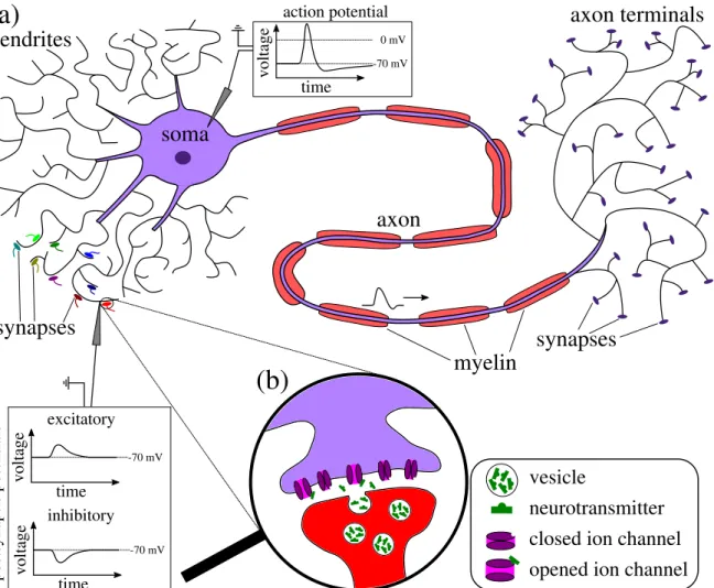
When the membrane voltage is sufficiently increased, the interplay of fast opening and clos- ing sodium channels and slower potassium channels yields a steep rise and a subsequent drop of the membrane potential that is referred to as action potential or spike. Within a neuron, action potentials are spatially transmitted to the axon terminals, at which chemical synapses are located that are one-way connections between the nerve cells. Note that some neurons are also electrically connected via gap junctions. When a chemical synapse is activated by an incoming action potential of the presynaptic neuron, vesicles are transported towards the synaptic cleft where they release neurotransmitters as illustrated in Fig. 1.2b. In turn, these neurotransmitters may bind to receptors on the postsynaptic side and open ion channels, yielding a change of the postsynaptic neuron’s potential. Neurons are characterized as exci- tatory or inhibitory depending on whether their synapses increase or decrease the membrane voltage of the postsynaptic cells, respectively.
Depending on their location and their specific task, neurons may drastically differ in their morphology, however, most of them have some common features that are illustrated in Fig. 1.2a. They consist of three different compartments, the dendrites, the cell body also known as the soma and the axon at the end of which are the nerve terminals. The dendrites are branched extensions from the nerve cell with the primary objective of receiving electrical signals from other neurons’ synapses and transmitting these to the cell body. There is also evidence that dendrites play a crucial role in certain computations [see for instance London and Häusser (2005); Sjöström et al. (2008); Schmidt-Hieber et al. (2017)]. The cell body con- tains the nucleus with the deoxyribonucleic acid (DNA) and all organelles that are required for the neuron to survive, however, it represents less than ten percent of the cell’s volume.
Originating from the soma, the axon is a long fiber used to transmit action potentials over relatively long distances. To speed up the propagation of action potentials over long distances and to save energy, parts of some axons are wrapped with myelin that serves as an isolation between intra- and extracellular domains. The axon branches into a large number of smaller fibers at the end of which synapses may be located to connect to other neurons.
Sources of noise that affect membrane voltages and signal transmission
Even if only a constant input current is applied, spikes of in vivo and in vitro neurons occur at irregular times, suggesting that the membrane voltage is subject to different sources of noise (Holden, 1976; Gerstner et al., 2014). There are mainly two intrinsic sources of noise: first of all, the membrane voltage is always subject to thermal noise, also known as Johnson-Nyquist noise (Johnson, 1928; Nyquist, 1928), however, its effect is negligibly small compared to the other fluctuations (Manwani and Koch, 1999). The more important source of intrinsic noise arises due to the finite number of ion channels in the cell membrane [see White et al. (2000) for review]. In the simplest case, channels assume either of two states, they are either open for ions to cross or closed and may switch stochastically. Note that
soma
axon dendrites
axon terminals
myelin
synapses synapses
vesicle
neurotransmitter closed ion channel opened ion channel
voltage time
action potential
-70 mV 0 mV
voltage time
-70 mV
voltage time
-70 mV
excitatory
inhibitory
postsynaptic potentials
(a)
(b)
Figure 1.2.: Sketch of a nerve cell (a) and a chemical synapse (b). Neuron (a): the dendrites receive electrical signals by synapses from other neurons and transmit them to the soma. Sufficient increase of the membrane voltage in the soma yields an action potential being a rapid increase and subsequent decrease of the membrane voltage that can be transmitted over long distances by the axon. For a faster propagation of action potentials, parts of the axon may be surrounded by myelin. The axon branches into many smaller fibers at which synapses are located.
Chemical synapse (b): an activated synapse releases neurotransmitter in the synaptic cleft that may bind to receptors and open postsynaptic ion channels yielding an increase or decrease of the postsynaptic potential, depending on whether the presynaptic neuron is excitatory or inhibitory, respectively.
some ion channels are much more complex and may assume several states. Although the number of ion channels per neuron is large, the fraction of open ion channels fluctuates and with it the membrane conductance and voltage. Concerning the membrane voltage of in vivo neurons in the cerebral cortex that are embedded in networks, spontaneous activity of the surrounding neural population is by far the dominating source of fluctuations (Destexhe and Rudolph-Lilith, 2012). These neurons are permanently exposed to the spikes of many presynaptic neurons, even if no sensory input is applied. Although these spikes may contain information, their effect on the membrane voltage is, comparable to noise, unpredictable on a small time scale and, thus, it is common to regard them as synaptic noise and model them as a stochastic process (Destexhe et al., 2003). Remarkably, synaptic noise may also occur in fully deterministic network simulations with randomly connected neurons due to the chaotic spiking behavior in such a complex system [see for instance van Vreeswijk and Sompolinsky (1996); Amit and Brunel (1997); van Vreeswijk and Sompolinsky (1998); Brunel (2000)].
Apart from that, the release of neurotransmitters by synapses with incoming action potentials is unreliable and measurements suggest that only a lower fraction of presynaptic spikes affect the postsynaptic potential (Hessler et al., 1993; Markram and Tsodyks, 1996). Note that noise does not need to be harmful to the transmission of signals, but, counterintuitively, noise may also be beneficial in nonlinear systems, a phenomenon well known in statistical physics as stochastic resonance [described for IF neurons by Longtin (1993), see also Gammaitoni et al.
(1998) and Lindner et al. (2004) for reviews].
1.3 Models of stochastic spiking neurons
To reach the goal of understanding how the brain works, studying of neural dynamics by means of appropriate mathematical models is inevitable. One of the most important in- sights that shaped the modern conception of neuronal functionality has been gained by the quantitative description of the membrane voltage in the squid’s giant axon by Hodgkin and Huxley (1952). In this famous model, the consideration of currents that arise due to the opening and closing dynamics of microscopic sodium and potassium ion channels resulted in a four-dimensional neuron model that was capable to adequately describe the generation and the shape of action potentials measured in voltage-clamp experiments. To account for further neural characteristics, the model has been extended by incorporating additional ion channels, the spatial extension, different compartments, other effects that arise due to the complex morphology and detailed synaptic dynamics [see summaries in Koch (1999); Dayan and Abbott (2001); Gerstner et al. (2014)] and detailed computer reconstructions of in vivo neurons have been made [see for instance Markram et al. (2015)]. If sufficient information on an experimental neuron is available, such detailed models can be fitted and may accurately reproduce neural activity. However, due to their complexity and their dependence on many parameters, these models are difficult to treat analytically and it is difficult to gain further insights in them. Furthermore, the power of detailed models which aim to mimic biologi- cal reality is limited for various reasons [see Almog and Korngreen (2016)]. To study the influence of general features on neural dynamics and computational properties of neurons, minimal models may be advantageous.
v
thv
r(a) (b)
spike train
Figure 1.3.: Trajectories of the leaky IF neuron with corresponding spike trains:
deterministic dynamics withµ=30 mV andβ= 0 (a) and neuron in the noise-driven regime with µ= 15 mV< vth andβ=1 mV√
s (b). Threshold and reset are indicated as dashed red and green lines. Other parameters: vr= 0mV,vth=20 mV,τref=5 ms,τm=20 ms.
In cases in which only the timing of the action potential is important and its detailed shape is not relevant, integrate-and-fire (IF) neurons are a powerful alternative since they are easy to implement and even provide analytical insights. Dating back to Lapicque (1907), they provide a phenomenological description of spiking neurons by a drastic simplification of the action potential generation. In general, IF neurons are given by the dynamics of the membrane voltage and a fire-and-reset rule:
τmv˙ =f(v, t), ifv(tk)> vth : v(tk+τref)→vr. (1.13) Here τm is the membrane time constant, f(v, t) incorporates both intrinsic dynamics and currents due to ion channels or applied by the experimentalist. When the voltage exceeds the threshold, the neuron is in a refractory state during the absolute refractory period τref.
The influence of fluctuations on the neural spike trains has been studied for the stochastic leaky IF neuron that arises by the choice of f(v) = −v+βξ(t). In this model, the leak current incorporated by −v ensures that the membrane voltage saturates at a certain value, if no other currents are applied. Neural input is given by the constant mean µ and white noiseβξ(t) [see for instance Gerstein and Mandelbrot (1964); Ricciardi (1977); Kistler et al.
(1997); Fourcaud and Brunel (2002) and Burkitt (2006a,b) for a review]. Two trajectories of this neuron model are presented in Fig. 1.3 for deterministic dynamics (β = 0) in Fig. 1.3a and for stochastic dynamics in the fluctuation-dominated regime (µ < vth) in Fig. 1.3b.
Analytical insights in this model have been gained in the above mentioned references by the application of the Fokker-Planck equation that reads in this special case:
∂tP(v, t) =−∂v
−v+µ τm P(v, t)
+ β2
2τm2 ∂2vP(v, t) +J(vth, t−τref)δ(v−vr) (1.14)
[cf. Eq. (1.11)]. Here the probability current term incorporates the reset of probability that crossed the threshold att−τref. The probability density obeys natural boundary conditions forv→ ∞and absorbing boundary conditions at the threshold:
v→−∞lim P(v, t) =P(vth, t) = 0. (1.15) The latter is a consequence of the white noise input as shown in detail in Sec. (5.7) of the book of Cox and Miller (1965). By the solution of Eq. (1.14) to a given initial distribution P(v,0), the probability density for a neuron to cross the threshold at time tis given by the efflux of probability caused by the absorbing boundary conditionJ(vth, t). The approach has first been used by Gerstein and Mandelbrot (1964) to analytically determine the interspike- interval distribution, that in turn could be used by Lindner et al. (2002) to calculate the spike-train power spectrum. Note that neuron models with multiplicative noise yields a different Fokker-Planck equation [see Richardson (2004)].
One-dimensional IF neurons are simple models that may provide a description of spon- taneous spiking activity, however, they cannot capture all neural features that have been observed in experiments. Such features require nonlinear and/or multidimensional IF neu- rons for which I develop a framework to determine the spike-train statistics, particularly the spike-train power spectrum, based on the corresponding Fokker-Planck equation in the following chapter.
multidimensional integrate-and-fire neurons
Stochastic one-dimensional integrate-and-fire (IF) neurons have been extensively used to study the effect of noise on spike trains. However, often they do not suffice to capture observed features of sensory neurons. For instance, in vitro neurons may have oscillatory properties (Puil et al., 1986; Gutfreund et al., 1995), emit spike-trains with negative interval correlations (Ratnam and Nelson, 2000; Chacron et al., 2000; Farkhooi et al., 2009; Avila- Akerberg and Chacron, 2011) or exhibit a complex spiking behavior as response to a constant input current (McCormick et al., 1985; Kawaguchi, 1993; Markram et al., 2004) whereas spike- trains of the corresponding one-dimensional IF neurons with constant input current and white noise are by construction renewal processes without memory. Fortunately, the number of applicable cases for IF neurons as models of real nerve cells increases, if they are extended towards multidimensional models. For instance, only one additional adaptation variable enables IF neurons to generate spike-trains with the above mentioned resonance properties (Richardson et al., 2003; Brunel et al., 2003) and negatively correlated intervals (Liu and Wang, 2001; Chacron et al., 2001). If they are combined with nonlinear voltage dynamics, these two-dimensional neurons may also show the observed spike patterns (Izhikevich, 2003, 2007; Touboul and Brette, 2008), furthermore, Brette and Gerstner (2005); Jolivet et al.
(2008); Teeter et al. (2018) have shown that they may accurately predict neural responses to noisy stimuli. Also effects that arise due to the morphology have been studied by IF neurons with multiple compartments, for instance by Ostojic et al. (2015); Doose et al. (2016).
While in all mentioned examples the further dimensions model intrinsic neuronal properties, they may also be exploited to generate temporally correlated fluctuations as neural input.
One source of such temporal correlations arises from the consideration of synaptic dynamics in a second variable. A popular model, studied for instance by Brunel and Sergi (1998);
Middleton et al. (2003); Lindner (2004); Moreno-Bote and Parga (2004, 2006); Schwalger and Schimansky-Geier (2008), considers synaptically filtered white Gaussian noise as neural input which yields IF models driven by an Ornstein-Uhlenbeck process. Such a one-dimensional embedding of white noise produces low-pass filtered Gaussian fluctuations also regarded to as red noise. But colored noise is required beyond this approach. Neural input in a network emerges as the sum of many presynaptic spike trains that my be approximated by Gaussian fluctuations. Most studies only apply white noise and suppose that spike-trains are close to Poisson processes. By that, they ignore the fact that spike trains are characterized by non- trivial temporal correlations, e.g. measuredin vivo by Ghose and Freeman (1992); Edwards
et al. (1993); Bair et al. (1994). Since neural input maintains the correlations of the single spike trains, as shown by Lindner (2006), a Gaussian approximation with colored noise is more accurate and may yield qualitatively different results, as for example shown for the synchronization behavior in a feed-forward network by Câteau and Reyes (2006). Markovian embeddings, of which the most popular examples are Ornstein-Uhlenbeck processes, may generate not only red noise, but a variety of colored noise that increases with the embedding’s dimensionality (Hänggi and Jung, 1995). For instance, a two-dimensional process have been used to generate band-pass-filtered noise, so-called harmonic noise (Schimansky-Geier and Zülicke, 1990), that served as neural input in order to study the electroreceptors of the paddlefish (Bauermeister et al., 2013).
The extension towards multidimensional models of course increases their complexity. Dur- ing the last decades, many studies have been concerned about special cases of multidimen- sional IF neurons and calculated their statistics either numerically (Casti et al., 2002; Au- gustin et al., 2017), semianalytically (Câteau and Reyes, 2006; Apfaltrer et al., 2006), analyt- ically by certain approximations (Brunel and Sergi, 1998; Brunel et al., 2001; Fourcaud and Brunel, 2002; Lindner, 2004; Moreno-Bote and Parga, 2010; Alijani and Richardson, 2011;
Schwalger and Lindner, 2015; Schwalger et al., 2015), or populations of IF neurons by the reduction to mesoscopic equations (Deger et al., 2014; Schwalger et al., 2017). Most of the studies consider equations for the dynamics of the probability density with an instantaneous reset after firing and derive the firing rate or interval statistics from them. In this chapter, a general framework for multidimensional IF neurons with a finite refractory period is intro- duced based on the corresponding multidimensional Fokker-Planck equation to calculate not only firing rate, but, more importantly, also the spike-train power spectrum.
Experimentally measured power spectra provide insights in the underlying neuronal dy- namics. Its low- and high-frequency limits are equal to the Fano factor of the spike train and the stationary firing rate, respectively. A high amplitude of peaks at the firing rate and its higher harmonics are an indicator of regular tonic firing caused by a strong constant stimulus.
Other peaks may reveal frequencies of subthreshold oscillations, of a periodic driving signal or of narrow-band noise as input. Edwards et al. (1993) have shown that certain mechanisms such as absolute refractory periods decrease long-term variability and yield reduced power at low frequencies. Such as experimental neurons, multidimensional neurons may emit spike- trains with a rich correlation structure. With help of these models, the influence of single neural features, but also the combination of several ones on the shape of the spike-train power spectrum can be studied. Hence, if we understand the spike-train power spectra of multi- dimensional IF neurons, we gain understanding of the occurrence of temporal correlations in real neurons.
Moreover, the calculation of the spike-train power spectrum of IF neurons driven by colored noise is of particular interest to understand the dynamics of neural networks. As already mentioned, neural input in networks maintains the temporal correlations of the presynaptic spike trains. Thus, in a homogeneous network, the temporal statistics of neural input and output are self-consistent, more precisely, the input spectrum and the spike-train spectrum are connected by a condition of self-consistency that is given by the network topology and the synaptic dynamics. In order to determine the self-consistent temporal correlations, an
troduced. The additional dimensions can be used to include common intrinsic features such as an adaptation current and/or further neuronal compartments and/or, to generate temporally correlated input fluctuations, so-called colored noise by a Markovian embedding.
iterative scheme was proposed by Lerchner et al. (2006) and improved by Dummer et al.
(2014) that was exploited by Wieland et al. (2015) to understand the amplification of slow fluctuations in neural networks. In this chapter, the preparatory work for a mean-field theory that considers the temporal correlations of spike trains is performed by the solution of the open-loop problem: the spike-train power spectrum is calculated for a given input power spectrum. In the next chapter, such a mean field theory is introduced based on the closed loop problem: the input power spectrum is searched that is self consistent with the corresponding spike-train power spectrum.
This chapter is organized as follows: at first, a comprehensible generalized two-dimensional IF model with absolute refractory period is introduced that involves many common features of IF neurons such as colored noise as neural input, an adaptation current or a second neuronal compartment. It is demonstrated how the non-local dynamics of this model, i.e. the fire-and- reset mechanism and spike-triggered adaptation, can be incorporated in the Fokker-Planck equation. From the Fokker-Planck equation, I derive a set of partial differential equations of which the solution determines the firing rate, the subthreshold probability density and, most importantly, the spike-train power spectrum. The set of equations is solved numerically by a finite-difference method for two important examples, a leaky IF neuron driven by colored noise and an exponential IF neuron with adaptation. As the second step, the model and the framework are extended toddimensions. The resulting set of partial differential equations is the highlight of this chapter and the preparatory work for the next one. As one example of a three-dimensional neuron, the theory is applied to calculate the power spectrum of a leaky IF neuron driven by narrow-band noise. At the end of this chapter, I introduce and test a procedure to determine the Padé approximation of the power spectrum at zero frequency. In this chapter, all calculated spike-train power spectra are verified by direct simulations of the corresponding Langevin equations.
2.1 The generalized two-dimensional integrate-and-fire neuron
For the sake of better comprehensibility, at first I consider a general two-dimensional IF neuron model for which the membrane voltage v and an auxiliary process a evolve in the subthreshold regime according to the general Langevin equations:
τmv˙=f(v, a) +βξ1(t),
τaa˙ =g(v, a) +b1ξ1(t) +b2ξ2(t). (2.1) The time scales of the dynamics are determined by the membrane and the auxiliary time constantsτm andτa, respectively. Both dynamics may influence each other via the functions f(v, a) and g(v, a). Here we restrict us to functions that ensure that neither v diverges towards−∞noradiverges towards±∞such that a stationary ensemble distribution exists.
Note that unrestricted increase of vis prevented by the fire-and-reset rule introduced below.
The terms ξ1(t) andξ2(t) are independent Gaussian white noise with zero mean hξi(t)i= 0 that obey the correlation hξi(t)ξj(t+τ)i =δi,jδ(τ) with i, j ∈ {1,2}. Here, the symbol δi,j
denotes the Kronecker delta. The coefficients β and b1 are noise strengths of the same white noiseξ1(t); the advantage of this construction will be explained later on. For all IF neurons the action potentials are generated artificially by the fire-and-reset rule: the neuron emits a spike when the voltage variable crosses the threshold vth at time tk. Here the shape of the action potentials is roughly approximated by a rectangular pulse that is formed due to the clamping of the voltage variable to the refractory voltage vref > vth during the absolute refractory period τref. After the refractory period has elapsed, the voltage is reset to vr and continues to evolve according to Eq. (2.1). Spike-triggered adaptation can be incorporated by the instantaneous increase of the auxiliary variable a(tk) by the constant amountδa:
ifv(tk)> vth: v(tk+τ) =vref for 0< τ < τref,
v(tk+τref)→vr and a(tk)→a(tk) +δa. (2.2) The representation of the action potentials by rectangular pulses is uncommon in the literature. In the most studies, the combination of an absolute refractory period and a voltage dependent auxiliary variable is not considered, thus, the voltage during the refractory period is irrelevant and clamped atvr[see for instance Burkitt (2006a)]. However, here the auxiliary variable may depend on the voltage via the function g(v, a), and hence, the effect of an increased voltage during the action potential may be included. The sequence of the action potentials at the spike times tk is represented as a stochastic point process, the spike train:
x(t) =X
k
δ(t−tk). (2.3)
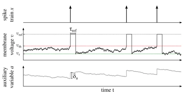
The trajectories of v and awith the resulting spike trainx for one example are presented in Fig. 2.2. In the following, I introduce statistics that are used to quantify the characteristics of the spike trains in this thesis.
time t auxiliary variable amembrane voltagevspike train x
δ
aτ
refvth
vr
vref
Figure 2.2.: Features of the two-dimensional integrate-and-fire neuron. From top to bottom: resulting spike train as a point process, membrane voltage and auxiliary dynamics that obey the subthreshold dynamics in Eq. (2.1) and the fire-and-reset rule in Eq. (2.2). When v exceedsvth, a spike is emitted and a is incremented by δa. Subsequently v is clamped to vref
during the absolute refractory periodτrefand is reset tovrafterwards. In this example,ais used as an stochastic adaptation current with spike-triggered and stochastic subthresholds adaptation as explained in detail in Sec. (2.1.4) withf(v, a) =µ−v−a,g(v, a) =Av−a. See Tab. C.2 in Appendix for parameters.
2.1.1 Spike-train statistics of first and second order
The number of spikes of a certain spike train x(t) within a time window [T0, T] is given by thespike count Nspikes(T0, T):
Nspikes(T0, T) =
T
Z
T0
dt x(t). (2.4)
The number of spikes per time unit is given by the firing rate. Theinstantaneous firing rate at a certain time r(t) is given by the expectation value of the number of spikes within an infinitesimally small time interval ∆t:
r(t) = lim
∆t→0
Nspikes(t−∆t/2, t+ ∆t/2)
∆t
= lim
∆t→0
* 1
∆t
t+∆t/2
Z
t−∆t/2
dt x(t) +
=hx(t)i. (2.5)
The expectation value is the ensemble average over realizations of the noise and the last step only holds true for an infinite ensemble size. The stationary firing rater0 denotes the firing rate of an ensemble with time-independent averages. The temporal correlations up to the second order are represented by theautocorrelation function that only depends on the time
lag τ and not on the absolute time tfor a stationary ensemble1:
C(τ) =hx(t+τ)x(t)i − hx(t)i2 =r0(δ(τ) +m(τ)−r0) (2.6) [see Holden (1976) or Gabbiani and Koch (1998) Sec. 6]. The function m(τ) denotes the firing rate under the condition that a reference spike is emitted at τ = 0. The reference spike itself is taken into account by the δ function such that m(0) = 0. Alternatively to the autocorrelation function, the temporal correlations are captured by the spike-train power spectrum given by:
S(ω) = lim
T→∞
hx(ω)˜˜ x∗(ω)i
T , x(ω) =˜
T
Z
0
eiωt[x(t)−r0]dt. (2.7) To be precise, we consider the power spectrum of the spike-train minus its expectation value r0in order to avoid the divergence of the spectrum atω = 0. The spike-train power spectrum as it is introduced here is connected to the autocorrelation function via the Wiener-Khinchin theorem by the Fourier transformation:
S(ω) =
∞
Z
−∞
dτ eiωτC(τ) =r0
1 + 2Re
∞
Z
0
dt eiωτ(m(τ)−r0)
(2.8)
[cf. Gardiner (1985) Eq. 1.5.38]. Here Eq. (2.6) and symmetry of the autocorrelation function [C(τ) =C(−τ)] are exploited in order to calculate the power spectrum by the real part of the integral over the positive half space. In the following section, an analytical set of equations is derived to calculate the stationary firing rate and the spike-train power spectrum. Note that in this work, the power spectra are plotted against the frequency f =ω/(2π) and not against the angular frequency ω, if not stated otherwise.
2.1.2 Fokker-Planck equation and spike-train power spectrum
Corresponding to the set of Langevin equations in Eq. (2.1) that describe single subthreshold trajectories of the model, the Fokker-Planck equation describes the temporal evolution for an entire ensemble of neurons. For the introduced model, the probability density P(v, a, t) to find a neuron with voltagev, auxiliary valueaat timetobeys the Fokker-Planck equation that is given by the operators ˆL and ˆR that incorporate the subthreshold dynamics and the fire-and-reset rule, respectively:
∂tP(v, a, t) = ˆLP(v, a, t) +{RˆP}(v, a, t). (2.9) In our model, a non-vanishing white noise component in the voltage variable is considered (β6= 0) which has infinite variance. As a consequence, neurons cannot be arbitrarily close to
1Non-stationary ensembles have time-dependent autocorrelation functionsC(t, τ) and are not considered in this work.