Bank finance versus bond finance

SFB 649 Discussion Paper 2005-042

Bank finance versus bond finance: what explains the differences between US and Europe?

Fiorella De Fiore*

Harald Uhlig**

* European Central Bank

** Humboldt-Universität zu Berlin, Deutsche Bundesbank, CentER and CEPR

This research was supported by the Deutsche

Forschungsgemeinschaft through the SFB 649 "Economic Risk".

http://sfb649.wiwi.hu-berlin.de ISSN 1860-5664

SFB 649, Humboldt-Universität zu Berlin Spandauer Straße 1, D-10178 Berlin

S FB

6 4 9

E C O N O M I C

R I S K

B E R L I N

Bank …nance versus bond …nance: what explains the di¤erences between US and Europe?

Fiorella De Fiore^y European Central Bank

Harald Uhlig^z

Humboldt Universität zu Berlin, Deutsche Bundesbank, CentER and CEPR This version: 1 August 2005

Abstract

We present a dynamic general equilibrium model with agency costs, where heterogeneous

…rms choose among two alternative instruments of external …nance - corporate bonds and bank loans. We characterize the …nancing choice of …rms and the endogenous …nancial structure of the economy. The calibrated model is used to address questions such as: What explains di¤erences in the …nancial structure of the US and the euro area? What are the implications of these di¤erences for allocations? We …nd that a higher share of bank …nance in the euro area relative to the US is due to lower availability of public information about

…rms’credit worthiness and to higher e¢ ciency of banks in acquiring this information. We also quantify the e¤ect of di¤erences in the …nancial structure on per-capita GDP.

JEL Classi…cation: E20, E44, C68.

Keywords: Financial structure, agency costs, heterogeneity.

The views expressed here do not necessarily re‡ect those of the European Central Bank or the Eurosystem.

We thank participants at the SED meetings, at the conferences on Dynamic Macroeconomics in Hydra, on DSGE Models and the Financial Sector in Eltville, on Competition, Stability and Integration in European Banking in Brussels, and seminar participants at Bocconi University. We are grateful to our discussants, Jajit Chada, Nobuhiro Kiyotaki, Andreas Schabert and Javier Suarez. This research was supported by the Deutsche Forschungsgemeinschaft through the SFB 649 “Economic Risk” and by the RTN network MAPMU.

yDirectorate General Research, European Central Bank, Postfach 160319, 60066 Frankfurt am Main, Ger- many. Email: …orella.de_…ore@ecb.int. Ph: +49-69-13446330.

zSchool of Bus. & Econ., WiPol 1, Humboldt University, Spandauer Str. 1, 10178 Berlin, Germany. Email:

uhlig@wiwi.hu-berlin.de. http://www.wiwi.hu-berlin.de/wpol. Ph: +49-30-2093 5927.

1 Introduction

This paper looks at the composition of the corporate sector’s external …nance as an important dimension through which credit market imperfections a¤ect the macroeconomy. In the pres- ence of agency costs, …nancial intermediaries provide contractual arrangements that reduce the e¤ects of information asymmetries between lenders and borrowers. This is achieved by o¤ering alternative …nancing instruments that best …t the needs of individual borrowers. Each instrument di¤ers in the cost imposed to lenders and borrowers and in the ability to reduce the macroeconomic e¤ects of information asymmetries.

Empirical evidence suggests substantial di¤erences in the …nancial structure across coun- tries. For instance, the traditional distinction between bank-based and market-based …nancial systems applies to the euro area and the US. Investment of the corporate sector relies much more heavily on bank …nance in the euro area than in the US. In 2001, bank loans to the corporate sector amounted to 42.6 percent of GDP in the euro area, and to 18.8 percent in the US. Conversely, outstanding debt securities of non-…nancial corporations and stock market capitalization amounted respectively to 6.5 and 71.7 percent in the euro area, and to 28.9 and 137.1 percent in the US.¹

In this paper, we introduce heterogeneous …rms and alternative instruments of external

…nance in a dynamic general equilibrium model with agency costs. We characterize the optimal choice of …rms among alternative instruments and derive the endogenous …nancial structure.

The model can be used as a laboratory to answer questions such as: What generates di¤erences in …nancial structures among countries? What are the implications of these di¤erences for allocations?

Existing models with agency costs (e.g. Kiyotaki and Moore (1997), Carlstrom and Fuerst (1997, 1998, 2001), Bernanke, Gertler and Gilchrist (1999), Christiano, Motto and Rostagno (2004) and Faia (2002)) do not allow to explain observed di¤erences in …nancial structures, as they do not distinguish between alternative instruments of external …nance. We introduce two types of …nancial intermediaries - commercial banks and capital mutual funds - into an other- wise standard model with credit frictions and information asymmetries. Each type of …nancial intermediaries (here onwards FIs) o¤ers a di¤erent intra-period contractual arrangement to provide external …nance to …rms. Firms experience a sequence of idiosyncratic productivity

1See Ehrmann et al (2003), Table 14.1.

shocks, the …rst being realized before …rms take …nancing decisions. Therefore, when choosing the source of external …nance …rms are heterogeneous in the risk they face of defaulting at the end of the period. Banks and capital mutual funds (CMFs) di¤er because banks are willing to spend resources to acquire information about …rms in …nancial distress, while CMFs are not. Conditional on the information obtained, banks give …rms the option to obtain loans and produce or to abstain from production and keep their initial net worth (except for an infor- mation acquisition fee to be paid to banks). The fact that banks spend resources to acquire information implies that bond …nance is less costly than bank …nance. Nonetheless, …nancing through bonds is a risky choice for …rms, because a situation of …nancial distress can only be resolved with liquidation and with the complete loss of the …rm’s initial net worth.

The contribution of the paper is twofold. First, we present a dynamic general equilibrium model where the …nancial structure of the economy can be endogenously derived from the …rms’

optimal choice of the …nancing instrument. Our model can easily embed …rms’heterogeneity in the risk of default without giving up tractability. The dynamics of the economy can be described by a system of aggregate equilibrium conditions similar to those arising in models without such heterogeneity. Second, we calibrate the model in steady state to replicate key di¤erences in the …nancial structure of the US and the euro area. We …nd that a higher share of bank …nance in the euro area relative to the US is due to lower availability of public information about …rms’credit worthiness and to higher e¢ ciency of banks in acquiring this information.

We also assess the quantitative importance of di¤erences in …nancial structures by comparing the observed ratios of per-capita GDP in versions of the calibrated model that allow for the use of one or two instruments of external …nance.

A related paper to ours is Carlstrom and Fuerst (2001). The main di¤erence is that in their model, …rms are ex-ante identical at the time of stipulating a …nancial contract.² Moreover, they have access to one …nancing instrument only. Therefore, in their framework it is not possible to address the importance of the composition of …rms’external …nance for the macroeconomy. Another di¤erence arises in the focus of the analysis. Carlstrom and Fuerst address the e¤ect of agency costs on the transmission of aggregate shocks. As our focus is

2In Calstrom and Fuerst (2001), at the time of the contract …rms can di¤er in terms of size. However, due to the speci…c characteristic of the contract solution, this type of heterogeneity is not relevant in equilibrium and …rms can be assumed identical ex-ante. In what follows, we will use the term ’ex-ante heterogeneity’ as implying heterogeneity at the time of the contract in the risk of defaulting at the end of the period. This type of heterogeneity is also relevant in equilibrium.

on the determinants of …nancial market structures, we restrict the attention to a steady state analysis.

Our paper also relates to recent theories of …nancial intermediation (e.g. Chemmanur and Fulghieri (1994) and Holstrom and Tirole (1997), among several others). We share with Chem- manur and Fulghieri (1994) the idea that banks treat di¤erently borrowing …rms in situations of …nancial distress because they are long-term players in the debt market while bondholders are not. Therefore, banks have an incentive to acquire a larger amount of information about

…rms. By minimizing the probability of their ine¢ cient liquidation, banks build a reputation for …nancial ‡exibility and attract …rms that are likely to face temporary situations of distress.

The steady state distribution of …rms arising in our model closely resembles that obtained by Holstrom and Tirole (1997) in a two-period model where …rms and intermediaries are capital constrained. The authors …nd that poorly capitalized …rms do not invest. Well capitalized

…rms …nance their investment directly on the market, relying on cheaper, less-information in- tensive …nance. Firms with intermediate levels of capitalization can invest, but only with the help of information-intensive external …nance.

The paper proceeds as follows. In section 2, we describe the environment and outline the sequence of events. In section 3, we present the analysis. We start by showing that in our economy the presence of agency costs translates into a …rm-speci…c markup that entrepreneurs need to charge over marginal costs. We proceed to derive the optimal contract between …rms and FIs, and we characterize the endogenous …nancial structure of the economy. We show that in each period, conditional on the realization of the …rst idiosyncratic shock, entrepreneurs split into three sets: entrepreneurs that decide to abstain from production, entrepreneurs that approach a bank and possibly obtain a loan, and entrepreneurs that raise external …nance through CMFs. Finally, we describe the consumption and investment decisions of entrepreneurs and households, present aggregation results and characterize the competitive equilibrium. In section 4, we illustrate the main properties of the model in steady state. In section 5, we review the evidence on di¤erences in the intermediation activities and in the …nancial structure of the corporate sector in the US and the euro area. Then, we present a calibration of the model that replicates in steady state the outlined key di¤erences. Finally, we explore possible reasons for such di¤erences and we look at the implications for allocations. In section 6, we conclude and outline our future research.

2 The Model

We cast the di¤erent role of corporate bonds and bank loans into a dynamic general equilibrium model with credit market frictions, where we maintain the assumption of one-period maturity of the debt.

The domestic economy is inhabited by a continuum of identical in…nitely-lived households, a continuum of heterogeneous …rms owned by in…nitely lived risk-neutral entrepreneurs, and two types of zero-pro…t FIs. Each …rm, indexed byi2[0;1];starts the period with an endowment of physical capital and with a constant returns to scale production technology that uses labor and capital as inputs. As the value of the initial capital stock is not su¢ cient to …nance the input bill, producing …rms need to raise external …nance.

In our model, two key ingredients allow to introduce a non-trivial choice of …rms among alternative instruments of external …nance. The …rst ingredient is the existence of two distinct types of FIs, where banks are willing to spend resources to acquire information about an unobserved productivity factor, while CMFs are not. The second key ingredient is a sequence of three idiosyncratic productivity shocks hitting each …rm. The …rst shock, "1;it; is publicly observed and realizes before …rms take …nancial and production decisions. The second shock,

"2;it;is not observed by anyone (not even the entrepreneur). Information on the realization of this shock can be acquired by the FIs at a cost that is proportional to the value of the …rm and then disclosed to the …rm in exchange of an up-front fee. The third shock, "3;it; realizes after borrowing occurs and is observable to the entrepreneur only. It can be monitored by FIs at the end of the period, at a cost that is a fraction of the …rm’s production. The …rst shock generates observable heterogeneity among …rms in the risk of default at the end of the period.

The second shock, in combination with the information acquisition role of banks, provides the rationale for choosing bank …nance for …rms facing high risk of default. The combination of these two shocks is crucial to generate cross-sectional variation in …rms’…nancing choices.

Finally, the third shock introduces asymmetric information and rationalizes the existence of risky debt as the optimal contract between lenders and borrowers.

Loans extended by both types of FIs take the form of intra-period trade credit calculated in units of the output good, as in Carlstrom and Fuerst (2001). Firms obtain labor and capital inputs from the households against the promise to deliver the factor payments at the end of the period. This requires a contractual arrangement, which is supplied by a FI.

2.1 The environment 2.1.1 Households

Households maximize the expected value of the discounted stream of future utilities, E₀

X1 t=0

t[lnct+ (1 lt)]; 0< <1; (1)

where is the households’discount rate,c_t is consumption,l_t denotes working hours and is a preference parameter. The households are also the owners of the FIs, to which they lend on a trade credit account to be settled at the end of each period. The representative household faces the budget constraints,

ct+kt+1 (1 )kt wtlt+rtkt; (2)

wherewt denotes the real wage andrtthe rental rate on capital.

2.1.2 Entrepreneurs

Each entrepreneurienters the period holding capitalz_it:The …rm operates a CRS technology described by

y_it="_1;it"_2;it"_3;itH_itK_it¹ ; (3)

where K_it and H_it denote the …rm-level capital and labor, respectively. The productivity shocks "1;it; "2;it and "3;it are random iid disturbances, which occur at di¤erent times during the period. They have mean unity,³ are mutually independent and have aggregate distribution functions denoted by 1; 2 and 3 respectively. Per independence assumption, these are also the marginal distributions. The entrepreneur faces the constraint that the available funds,x_it, need to equal the costs of renting the factors of production;

xit=wtHit+rtKit: (4)

Entrepreneurs are in…nitely lived, risk-neutral and more impatient than households. They discount the future at a rate , where is the discount factor of households and0< <1.

Entrepreneurial utility is linear in consumption and in e¤ort. Running a risky project requires an entrepreneurial e¤ort proportional to the size of the project, xit. De…ne Dit as a dummy

3An aggregate technology shock can be introduced by assuming that the mean"1t of the …rst entrepreneur- speci…c technology shock is not unitary.

variable that takes the value of 1 if …rm i produces in period t and of 0 if it does not. The problem is to maximize the expected value of the discounted stream of future utilities,

E₀ X1 t=0

( )^t(e_it x_itD_it); 0< <1; (5) subject to the budget constraint

eit+zit+1 =y_it^e; (6)

Heree_itdenotes entrepreneurial consumption,z_it+1 is investment in physical capital to be used in periodt+ 1;and y^e_it is the share of the …rm’s production accruing to the entrepreneur after repayment of the loans. The parameter measures the disutility of exerting e¤ort in running the project.

Notice that, because entrepreneurs are more impatient than households, they demand a higher internal rate of return to investment. This opens the room for trade between households and entrepreneurs despite the agency costs of external …nance.

2.1.3 Agency costs and …nancial intermediation

Entrepreneurs obtain labor and capital inputs from the households against the promise to deliver the factor payments at the end of the period. Given the possibility of default by …rms, this promise needs to be backed up by a contractual arrangement with a FI (a bank or a CMF). The competitive FIs are able to diversify the risk among the continuum of …rms facing idiosyncratic risk. Hence, they ensure repayment of the factors of production to the households despite the possibility of default by …rms. Since credit arrangements are settled at the end of the same period, the intermediaries break exactly even on average.

Let!it be the uncertain productivity factor at contracting time, when …rms approach FIs,

!_it= 8<

:

"_2;it"_3;it for CMF …nance

"3;it for bank …nance

Firms that decide to raise …nance from banks pay an up-front fee that covers the bank’s cost of information acquisition about the signal "_2;it: The fee is a …xed proportion of the …rm’s valuenit:This cost is not faced by …rms that sign a contract with CMFs, as these FIs do not acquire information about the unobserved shock. Hence, the disposable net worth of a …rm at the time of the contract is given byn~it;where

~ n_it=

8<

:

n_it for CMF …nance (1 )nit for bank …nance

Conditional on "1;it and possibly "2;it as described in section 2.2 below, each entrepreneur chooses to invest an amount0 bn_it n~_it of internal …nance in the risky project and requests an amountxit nbit of external …nance to a FI to back up his promise of repayment, for total funds at hand of x_it. Throughout the analysis, we assume that entrepreneurs cannot enter actuarily fair gambles with FIs.

Each FI is willing to …nance a project whose size is a …xed proportion of the internal funds invested,

x_it= nb_it; 1: (7)

This assumption captures the idea that entrepreneurs di¤er in their ability to run projects.

In particular, the maximal size of a project which an entrepreneur is capable of running is proportional to his net worth.

After the realization of the uncertain productivity factor, !_it; the entrepreneur observes the actual production in units of goods, y_it; and announces to the FI repayment of the debt or default. The realization of !it is only known to the …rm unless there is costly monitoring, which requires destroying a fraction of the …rm’s output. After the announcement of the entrepreneur, the FI decides whether or not to monitor.

The informational structure at contracting time corresponds to the costly state veri…cation (CSV) framework of Townsend (1979) and Gale and Hellwig (1985).⁴ A standard result of this framework is that the optimal contract between each …rm and FI is risky debt. The contract speci…es how to divide the …rm’s …nancing requirement into internal and external …nance. It also speci…es, for each announced output and prior information ("_1;it under CMF …nance and

"1;it"2;it under bank …nance), a threshold for the uncertain productivity factor, !it. The …rm defaults and the FI commits to monitor if the entrepreneur’s announcement of !_it is below this threshold. If there is monitoring,!it is made known to the FI and the …rm’s production is completely seized. The contract also sets a …xed repayment for …rms that do not default.

2.2 The timing of events

The following list provides an overview of the timing of events in period t:

4Restriction (7) is usually not imposed in the costly state veri…cation literature. It is necessary in our model economy to ensure that all …rms raise …nite amounts of external …nance, despite the presence of ex-ante heterogeneity. Such assumption and its consequences are discussed in greater detail in section 3.2.1.

Entrepreneurs and households enter the period holding respectively capitalzitandk_ht. House- holds plan, how much labor to supply, and how much consumption and investment goods to purchase. They also supply labor and rent out their capital stock. Entrepreneurs calculate the end-of-period value n_it of their capital holdingsz_it, which is publicly observable:

Financial decisions unfold over three stages.

I. The …rst entrepreneur-speci…c shock "_1;it is realized and publicly observed. Conditional on its realization, entrepreneurs decide whether to:

a. Abstain from production. Entrepreneurs facing a low "1;it;or a high risk of default, decide not to borrow and not to produce, i.e. they choosebn_it= 0. They rent out capital on the market, thus retaining their initial net worth,nit;until the end of the period.

b. Possibly borrow from banks and produce. Entrepreneurs facing an intermediate real- ization of"1;it decide to approach a bank and to postpone their production decision after the realization of the second productivity shock"_2;it:⁵

c. Borrow from CMFs and produce. Entrepreneurs facing a high realization of"_1;itdecide to raise external …nance from CMFs and not to acquire information on"2;it:

II. "_2;it is realized and not observed by anyone. Information on its realization is acquired by banks at a cost nit and communicated to entrepreneurs. Conditional on"2;it;entrepre- neurs choose their investment level 0 bn_it n~_it= (1 )n_it;i.e. whether to:

d. Abstain from production,in which case bn_it= 0. These entrepreneurs rent out capital, retaining their remaining net worth,(1 )nit;until the end of the period.

e. Borrow from banks and produce.

III. Entrepreneurs that have chosen to produce hire laborH_it and rent capital K_it from the households against the promise to deliver the factor payments at the end of the period.

5At this point, one could introduce the possibilities for entrepeneurs to enter actuarily fair gambles. It turns out that entrepreneurs would enter these gambles, and transfer their entire net worth to those entrepreneurs which draw the highest values of"2. Equivalently, one could assume that banks are allowed to cross-subsidize projects. They would take resources from low-"2 entrepreneurs and give them to high-"2 entrepreneurs. Here we e¤ectively outlaw gambling and cross-subsidization, as common in the literature. An assumption which can rule out the bene…ts of such gambles is su¢ cient risk aversion for the entrepreneurs. This, however, would substantially increase the complexity of the model.

This promise is backed up by the value of their own capital holdings plus the value of the additional trade credit obtained from the FI (either a bank or a CMF).

The third shock"_3;it is realized and observed by the entrepreneur only. Production takes place, yit = "1;it"2;it"3;itH_itK_it¹ . The entrepreneurs keep part of output, y_it^e; for own consumption and investment, and sell the rest to households to settle trade credit. En- trepreneurs announce the outcome of production and repay loans or default on loans, if they cannot repay the agreed-upon amount. Conditional on the announcement, the

…nancial intermediaries decide whether or not to monitor.

Entrepreneurs consumeeit and accumulate capitalzi;t+1. Households use the goods purchased for consumptionc_tand investment in capital k_h;t+1.

3 Analysis

First, we show that the presence of agency costs translates into a …rm-speci…c markup that entrepreneurs need to charge over marginal costs. Then, we characterize the contract between each …rm and FI, and we derive the endogenous …nancial structure. We proceed by charac- terizing consumption and investment decisions of entrepreneurs and households. Finally, we present aggregation results and characterize the competitive equilibrium.

3.1 Factor prices and the markup

Each entrepreneur’s net worth, n_it; is given by the market value of his accumulated capital stock, z_it;calculated as the to-be-earned factor payments plus the depreciated capital stock,⁶

n_it= (1 +r_t)z_it; (8)

Firms that produce need to sign a contract with the FIs to raise external …nance for total funds at hand x_it. Normalizing goods prices, the …rm’s demand for labor and capital is derived by solving the problem

max E "_1;it"_2;it"_3;itH_itK_it¹ w_tH_it r_tK_it

6One possible interpretation is that entrepreneurs sell their capital stock at the beginning of the period against trade credit nit:Notice that entrepreneurs’ net worth should include also a …xed income component (e.g. a constant lump-sum subsidy ):This would ensure that, if the entrepreneur defaults in periodt 1, he can obtain external …nance and eventually produce. Since introducing a small constant subsidy does not a¤ect the analysis, we abstract from it.

subject to the …nancing constraint (4). Here the expectation E[ ] is taken with respect to the productivity variables yet unknown at the time of the factor hiring decision. More precisely,

E["_1;it"_2;it"_3;it] = 8<

:

"_1;it for CMF …nanced …rms

"1;it"2;it for bank …nanced …rms

Denote the Lagrange multiplier on the …nancing constraint assit 1. Optimality implies that

Kit = (1 )xit

r_t

Hit = xit

wt

E[yit] = sitxit: where

sit = 8<

:

"1;itqt for CMF …nance

"_1;it"_2;itq_t for bank …nance

(9)

q_t= wt

1 rt

1

: (10)

We can interpret qt as an aggregate distortion in production arising from the presence of agency costs in the economy. Notice that s_it acts as a markup, which …rms need to charge in order to cover the agency costs of …nancial intermediation. Moreover, sit is …rm-speci…c:

depending on what is already known about …nal …rm productivity, i.e. depending on "_1;it and (for bank-…nanced …rms) "2;it, the …nancing constraint may be more or less severe.⁷

3.2 Financial structure

In our model, the …nancial contract is intra-period but the game between …rms and FIs unfolds over three stages (described in section 2.2). To derive the endogenous …nancial structure, we solve the model using backward induction.

First, we derive the optimal choice of agents in stage III. Conditional on the available prior information ("1;it under bank …nance and"1;it"2;it under bank …nance), …rms and FIs stipulate a contract that is the optimal solution to a costly state veri…cation (CSV) problem.

Then, we characterize the optimal choice of agents in stage II. Firms that have signed contracts with banks acquire at a cost information about "_2;it; on the basis of which they decide whether or not to abstain from production. The decision is taken conditional on the

7In Carlstrom and Fuerst (2001), as in most of the literature, nothing is known before …rms produce, i.e., E["1;it"2;it"3;it] = 1andsit=qt.

solution of the game in stage III (the …nancial contract) and on the available prior information ("_1;it"_2;it). We characterize thresholds for the realization of the observed …rm-speci…c markup sit that determine the …rm’s decision of whether or not to borrow and to produce.

Finally, we characterize the optimal decision in stage I. Conditional on the solution of stage II and III (which provides expected pay-o¤ from producing when raising external …nance through banks or CMFs), …rms decide whether or not to produce and, if they do, which instrument of external …nance to use. We derive thresholds for the realization of the observed

…rm-speci…c markup s_it that determine the …rm’s decision. We show that these thresholds depend only on the distributional assumptions on the three idiosyncratic productivity shocks.

3.2.1 The costly state veri…cation contract

The solution to our CSV problem is a standard debt contract (see e.g. Gale and Hellwig (1985)) that is characterized by three properties. First, the repayment to the FI is constant in states when monitoring does not occur. Second, the …rm is declared bankrupt if and only if the …xed repayment cannot be honoured. Third, in case of bankruptcy, the FI commits to monitor and completely seizes the output in the hands of the …rm. The …rst and third properties ensure that the contract is incentive compatible. The second property ensures that monitoring is done in as few circumstances as possible to avoid the deadweight loss.

Let ! and '_! be respectively the distribution and density function of!it and recall that the presence of agency costs implies that y_it=s_it!_itx_it:De…ne

f !^j =

Z ₁

!^j

! !^j _!(d!) (11)

g(!^j) = Z !^j

0

! _!(d!) _! !^j +!^j 1 _! !^j (12)

as the expected shares of …nal output accruing respectively to an entrepreneur and to a lender, after stipulating a contract that sets the …xed repayment at s_it!^j_itx_it units of output; for

j =b; c. The index j denotes the type of FI, where b indicates banks andc indicates CMFs.

The optimal contract solves the following CSV problem:

max h

s_itf(!^j_it) i

x_it (13)

subject to constraint (7) and

sitg(!^j_it)xit xit bnit (14)

f !^j_it +g !^j_it 1 ! !^j_it (15)

b

nit 0; h

sitf(!^j_it) i

xit bnit (16)

The optimal contract maximizes the entrepreneur’s expected utility subject to the restriction on the project size, (7), the lender being willing to lend out funds, (14), the feasibility condition, (15), and the entrepreneur being willing to sign the contract, (16). Since loans are intra-period, the opportunity cost of lending for the intermediary equals the amount of loans itself,x_it bn_it: Notice that constraint (7) usually does not appear in the standard CSV setup. When …rms are identical in terms of default risk, the contract determines optimally the size of the project.

This latter turns out to be linear in net worth, as in our model. However, when …rms are identical the ratio of the project size to net worth depends on the threshold for the idiosyncratic shock and on the aggregate variable qt, while it is constant in our model. This implies that leverage is …xed in our environment. The reason for this assumption is that, with heterogeneity in the risk of default, …rms di¤er in terms of credit-worthiness. When the distribution of the idiosyncratic shock"_1tis unbounded, the optimal project size for …rms experiencing extremely large values of that shock would be unbounded. To avoid corner solutions in the allocation of funds from FIs, we set the project size to a …xed share of the …rm’s initial net worth. This assumption ensures that all …rms raise …nite amounts of external …nance.

Proposition 1 Under the optimal contract, the entrepreneur either invests nothing, nbit = 0;

or invest his entire net worth, bn_it = ~n_it; requiring an amount ( 1) ~n_it of external …nance.

The optimal contract is characterized by a threshold !^j_it; j=b; c, such that, if the entrepreneur announces a realization of the uncertain productivity factor ! !^j; no monitoring occurs.

If ! < !^j, the FI monitors at a cost and completely seizes the resources in the hands of the entrepreneur. The threshold is given by the solution to

s_itg(!^j_it) = 1

: (17)

Proof: Condition (7) and (16) imply that the expected utility of entrepreneurs willing to produce is not lower than the utility from disposing of the net worth initially invested. Notice that the problem is linear innbit:Thus, the solution is such that the entrepreneur either invest

nothing and does not produce, bnit = 0; or invest everything and produce, nbit = ~nit: Entre- preneurs that produce only raise costly external …nance to cover what is needed in excess of the internal funds,xit n~it= ( 1) ~nit:Expression (17) for the threshold!^j_it can be derived by observing that f(0) =R₁

0 ! _!(d!) = 1; g(0) = 0, f⁰(!^j_it) = h

1 _! !^j_it i

<0; and g⁰(!^j_it) >0:This latter property can be shown by contradiction. Suppose g⁰ !^j_it <0:Then, it would be possible to increase expected utility of the …rm, h

s_itf(!^j_it) i

~

n_it;by reducing

!^j_itwhile increasing expected pro…ts of the FI,sitg(!^j_it) ~nit:Hence,!^j_it could not be a solution to the contract. It follows that the unique interior solution to the problem is given by (17).

The terms of the contract can be written as

!^j_it=!^j(sit); j =b; c (18)

where sit satis…es (9). Notice that ^@!

j it

@sit = ^g(!

j it)

sitg⁰(!^j_it) < 0 and hence ^@!

j it

@qt < 0: The higher the …rm-speci…c mark-up s_it orq_t;the lower the threshold, !^j_it;below which the entrepreneur defaults and is monitored. Given the solution to the contract, we can de…ne the risk premium r_it^j as the interest rate charged for the use of external …nance. It is implicitly given by the condition (1 +r^j_it) (xit n~it) =sit!^j_itxit.

3.2.2 Bank loan continuation

At the beginning of stage II, the second productivity shock,"_2;it;is realized and not observed by anyone. Information on this shock is acquired by banks and communicated to the entre- preneur. Conditional on the realization of "_2;it; the entrepreneur chooses whether to abstain from production or to obtain trade credit and produce.

Proposition 2 A threshold forsit="1;it"2;itqt;below which the entrepreneur does not proceed with the bank loan, exists and is unique. It is given by a constant s_d that satis…es

h

s_itf(!^b(s_it)) i

= 1: (19)

Proof: Consider the situation of a …rm that, upon payment of the information acquisition fee, n_it; observes "_1;it and "_2;it. The entrepreneur proceeds with the bank loan if and only if his expected utility exceeds the opportunity costs of renting his capital to others, i.e. if s_itf(!^b(s_it)) 1;where s_it ="_1;it"_2;itq_t:Notice that expected utility from proceeding with the bank is negative forsit= 0 and strictly increasing insit;sincef⁰ !^b_it <0and ^@!_@s^bit

it <

0:Hence, a solution to condition (19), taken with equality, exists and is unique. Moreover, it is constant across …rms and time.

Consider for a moment an environment where banks are allowed to cross-subsidize …rms.

Each …rm would decide at the beginning of stage II whether or not to exchange its net worth for an actuarily fair gamble. The gamble would set an up-front fee and a repayment to the bank, which would depend on the prior available information,"_1;it, and the unobserved shock,"_2;it. In appendix A, we show that the optimal …nancial arrangement would be one where banks cross-subsidize …rms. With"_2;it below a certain threshold, the …rm would not produce but the bank would seize completely its net worth. With"2;it above that threshold, the …rm would get full funding at the lowest possible cost. Repayments of producing …rms would be minimized and so would be the probability of default and expected monitoring costs. The contract with cross-state subsidization would be optimal because it would minimize agency costs, increasing the aggregate resources available for entrepreneurial consumption and hence improving welfare of the risk-neutral entrepreneurs. It might be of interest to investigate the resulting general equilibrium e¤ects in such an environment. However, a frequent objection to contracts that allow for cross-state subsidization is that lotteries are not observed in …nancial markets. One possible explanation is that investors are risk-averse, an element that is neglected in standard models with agency costs. For this reason, we do not allow …rms to gamble:

3.2.3 The choice of the …nancing instrument

In stage I, after "1;it realizes, the entrepreneur chooses whether or not to produce and, if he does, how to …nance production. For notational simplicity, we drop the subscripts.

The expected utility of an entrepreneur, who proceeds with bank …nance conditional on the realization of "₁;isF^b(s)n, where s="₁q and

F^b(s) = (1 ) Z

sd s

s"2f(!^b(s"2)) 2(d"2) h

1 2(sd

s) i

+ 2(sd

s)

!

(20) The possibility for the entrepreneur to await the further news "₂ before deciding whether or not to proceed with the bank loan provides option value.

The expected utility of an entrepreneur, who proceeds with CMF …nance conditional on the realization of "1;isF^c(s)n, where s="1q and

F^c(s) = [sf(!^c(s)) ] : (21)

Finally, the expected utility of an entrepreneur, who abstains from production, is simply n. Note in particular, that all payo¤ functions are linear in net worthn.

Knowing its own mark-ups="1q, each entrepreneur chooses his or her best option, leading to the overall payo¤F(s)n, where

F(s) = maxf1;F^b(s);F^c(s)g: (22) Conditional on s, entrepreneurs split into three sets: _at, the set of entrepreneurs that abstain from raising external …nance in period t; bt; the set of entrepreneurs that sign a contract with banks, and _ct; the set of CMF-…nanced entrepreneurs. We show that these three sets are intervals in terms of the …rst idiosyncratic productivity shock "1.

In the analysis below, we assume that conditions (A1) and (A2) are satis…ed.

(A1)F^b0(s) 0;

(A2)F^b0(s)< F^c0(s);for alls="₁q:

Assumptions (A1) and (A2) impose mild restrictions on the parameters of the model. A su¢ cient condition for (A1) to be satis…ed is that '_"2(^s_s^d) < 1; since s_df(!^b(s_d)) = 1 + andf⁰(!^b)_@("^@!b

2s) >0:The condition imposed by(A2)is also mild. Intuitively, …rms with a low realization of the productivity shock"₁ (a lows) have expectations of low returns from under- taking production after signing a contract with the bank, as represented by the …rst two terms in brackets, in the expression for F^b(s):For those …rms, the gain from minimizing the possi- bility of liquidation, (1 ) 2(^s_s^d);is relatively more important. Ifs increases, the expected return from production increases both for bank- and for CMF-…nanced …rms. However, the increase is higher under CMF …nance because intermediation costs are lower. Hence, there will be a threshold above which expected pro…ts from production for CMF-…nanced …rms exceed those for bank-…nanced …rms. (A1)and (A2)ensure uniqueness of the thresholds s_b and s_c: Proposition 3 Under (A1), a threshold for s="1q, below which the entrepreneur decides not to raise external …nance, exists and is unique. It is given by a constant s_b that satis…es

F^b(s) = 1: (23)

Proof: Notice thatF^b(0) = 1 :Under (A1), there is a unique cuto¤ pointsb;which satis…es the conditionF^b(s) = 1:This point is constant across …rms and time.

Proposition 4 Under (A1) and (A2), a threshold for s="1q above which entrepreneurs sign a contract with the CMF, exists and is unique. It is given by a constant s_c that satis…es

F^b(s) =F^c(s): (24)

Proof: Notice that,F^b(0) = 1 > F^c(0):A su¢ cient condition for existence and uniqueness of a threshold s_c is provided by (A1) and (A2). The threshold is constant across …rms and time.

Conditional on q_t;entrepreneurs split into three sets that are intervals in terms of the …rst idiosyncratic productivity shock "1;it,

at = f"1;it j"1;it < sb=qtg

bt = f"1;it jsb=qt "1;it sc=qtg

ct = f"1;it j"1;it > sc=qtg

for some constantss_b,s_c. Notice that an increase inq_t raises expected pro…ts from producing, conditional on the realization of "_1;it, and reduces the thresholds s_b=q_t and s_c=q_t: Hence, it decreases the share of …rms that decide to abstain from production and increases the share of

…rms that sign a contract with FIs. Notice also that condition (19) determines a threshold s_d for the …rm-speci…c markup, below which …rms that have signed a contract with banks decide to abstain. A corresponding threshold for the second …rm-speci…c shock"2;it can be computed as s_d=(q_t"_1;it): Conditional on the realization of "_1;it; an increase in q_t reduces this threshold and the share of …rms that decide to abstain conditional on having signed a contract with a bank. The …rm’s decision on whether or not to produce can be characterized by

D_it = 8<

:

1if"1;it > sc=qt or ifs_b=qt "1;it sc=qtand "2;it > s_d="1;itqt

0 else 3.3 Consumption and investment decisions

Consumption and investment decisions of the households are described by the solution to the maximization problem (1) subject to (2), which is given by

ct = wt (25)

1 ct

= Et

1 ct+1

(1 +rt+1) : (26)

The entrepreneurial decision on consumption and on investment in capital, which will be used as net worth in the following period, derives from the maximization of (5) subject to (6), where y_it^e = ~nit if …rm i abstains, y_it^e = sit !it !^j_it n~it if …rm i borrows and repays, and y_it^e = 0 if …rm i borrows and default. The optimality condition is then given by the intertemporal Euler equation

1 = Etf(1 +rt+1)F("1;it+1qt+1)g: (27) Observe that qt+1 depends on wt+1 and rt+1 through (10). This equation ties down a rela- tionship between these two factor prices. It also pins down the evolution of net worth of the entrepreneurs, since they will elastically save and supply capital, so that factor prices satisfy this equation exactly period by period.

3.4 Aggregation

We are now ready to calculate aggregate variables. Given q_t and total entrepreneurial net worth n_t, we can compute total demand for funds, x_t;total output including agency costs, y_t; and total output lost to agency costs,y_t^a;by integrating across …rms. The conditions are:

x_t = ^x(q_t;s_b; s_c; s_d) n_t (28)

y_t = ^y(q_t;s_b; s_c; s_d)q_t n_t (29)

y_t^a = ^a(q_t;s_b; s_c; s_d) q_t n_t; (30)

where the functions ^x( ); ^y( ) and ^a( ) are de…ned in Appendix C.

Aggregate entrepreneurial consumption and investment have to satisfy the constraint

et+zt+1=#(qt;sb; sc; sd)nt; (31)

where the function #( ) is also de…ned in Appendix C.

Finally, aggregate factor demands are given by

w_tH_t = x_t (32)

r_tK_t = (1 )x_t: (33)

3.5 Market clearing

Market clearing for capital, labor and output requires that

K_t = k_t+z_t; (34)

Ht = lt; (35)

yt = ct+et+y_t^a+Kt+1 (1 )Kt: (36)

Market clearing for loans is ensured by condition (4), which equates the total funds available (i.e. the sum of internal and external …nance) to the demand of funds.

3.6 Competitive equilibrium

Given the process of the idiosyncratic shocks, f"1;it; "2;it; "3;itg; and the initial conditions (k₀; z₀); a competitive equilibrium consists of sequences of …rm-speci…c mark-ups, fs_itg¹t=0; threshold levels for the uncertain productivity factor !^b(sit); !^c(sit) ¹_t=0;constant thresholds for the …rm’s mark-upfs_b; s_c; s_dg¹t=0;production decisionsfD_itg¹t=0;demand functions for la- bor and capitalfHit; Kitg¹t=0;and consumption and investment decisionsfeit; zi;t+1g¹t=0;fori2 (0;1):It also consists of aggregate factorsfq_tg¹t=0;allocationsfc_t; l_t; H_t; K_t; e_t; x_t; y_t; y^e_t; y_t^ag¹t=0; laws of motion for the capital stocks fkt+1; zt+1g¹t=0;and pricesfwt; rtg such that:

Households maximize expected utility by choosingc_t; h_t andk_t+1;subject to the budget constraint, taking prices as given.

Entrepreneurs decide whether or not to produce: If they do, they choose Hit and Kit; to maximize pro…ts, subject to the production technology and the …nancing constraint, taking prices as given. Firm i; i 2 ^ct takes as given also the realization of the …rst idiosyncratic productivity shock, "_1;it. Firm i; i 2 bt takes as given the realization of

"1;it and "2;it. Entrepreneurs also choose consumption, ei;t; and investment, zi;t+1; to maximize their linear utility, subject to their budget constraint.

FIs and …rms solve a CSV problem. The solution determines the amount of external

…nance to be used and a threshold level for the uncertain productivity factor!^j_it; j=b; c:

When this factor is lower than the threshold, the …rm is monitored.

The market clearing conditions for goods, labor, capital and loans hold.

A competitive equilibrium is characterized by equations (8)-(12), (17) and (19)-(36).

4 Steady state properties: a numerical analysis

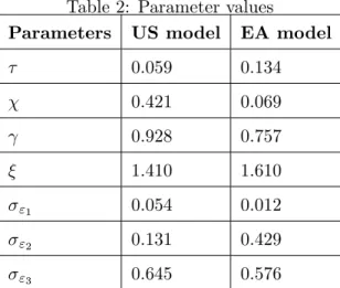
We parameterize the model at the stochastic steady state, which is characterized in Appendix B. The Appendix also describes the numerical procedure used to compute it. We assume that the iid productivity shocks v = "1; "2; "3 are lognormally distributed, i.e. log(v) is normally distributed with variance ²_v and mean ²_v=2. We set the discount factor at =:98 and the depreciation rate at = :025;⁸ leading to a real interest rate r = 4%. We choose = :64 in the production function and a coe¢ cient in preferences so that labor equal :3 in steady state, = 2:6: We set monitoring costs to be 15% of the …rm’s output, = :15; a value in the middle of the estimates in the empirical literature.⁹ We are then left with 7 free parameters, ; ; ; ; _"1; _"2 and _"3. In this section we …x them arbitrarily to show the qualitative properties of the model in steady state, i.e. = 1:6; = 0; = :11; = :704;

"1 =:26; _"2 =:46and _"3 =:13. In section 5 below, we calibrate the model and choose the

parameters to match stylized facts on the …nancial structure of the corporate sector in the US and in the euro area (here onwards EA).

In Figure 1, we show expected pro…ts for entrepreneurs. Panel (a) plots respectively ex- pected pro…ts from abstaining, from signing a contract with a bank and from signing a contract with a CMF, as a function of the …rm’s mark-up,s="1q. The intersection points of the three curves provide the cuto¤ points, s_b and s_c. The panel also shows the mean of the …rm-speci…c mark-up s; plus/minus two standard deviations. After the realization of"1;95% of the …rms’

markups lie within this region. Panel (b) shows how expected pro…ts from bank …nance move with the information acquisition fee :When = 0;expected pro…ts from bank …nance always exceed those from abstaining or from CMF …nance. All …rms raise external …nance through banks. When is large, the option value of acquiring more information is not large enough to o¤set the cost. All …rms either abstain or use CMF …nance. Only for intermediate values of

;…rms that decide to produce di¤erentiate in terms of their …nancing choice. They split into bank …nance and CMF …nance according to the realization of their markups.

8The annual depreciation rate is set to equal the US ratio of investment to capital over the period 1964-2001, as reported by Christiano et al (2004).

9Warner (1977) estimates small direct costs in a study of 11 railroad bankruptcies, with a maximum of 5.3% of the …rm’s value. Altman (1984) …nds that direct costs plus indirect costs (those related to the loss of customers, suppliers and employees, and the managerial expenses) are between 12.1% and 16.7%. Alderson and Betker (1995) provide the largest estimate, 36% of the …rm’s value.

Figure 2 illustrates the …nancial decisions of …rms. Panel (a) plots how …rms allocate among

…nancial instruments. Conditional on the value of the aggregate variableq; …rms experiencing a productivity shock"1 s_b=qdecide to abstain from production. Firms withs_b=q "1 sc=q sign a contract with banks:Firms with "₁ s_c=q sign a contract with CMFs. Among …rms that sign a contract with banks, those experiencing a productivity shock "2 s_d="1q decide not to proceed to the production stage. Panel (b) plots the thresholds_d="₁q;over the range of mark-ups(s_b=q; sc=q), as a function of"1:Panel (c) shows the probability that"2 s_d="1q;as a function of"₁:The larger"₁;the lower the threshold level for"₂ and the higher the probability that the …rm will produce, conditional on having signed a contract with a bank.

Figure 3 plots the steady state distribution of …rms among production activities. Firms that do not produce are those that decide not to raise external …nance because"1 s_b=q, and those that sign a contract with the bank but, after the realization of "₂, decide to drop out of production. For these …rms,s_b=q "1 sc=q and "2 s_d=q"1:

Figures 4 and 5 plot the results from a sensitivity analysis, which is carried out by modifying one parameter at a time. The …rst experiment is to look at the e¤ect of di¤erent entrepreneurial discount factors by changing the value of q. Notice from the steady state version of equation (27) that, for a given level of entrepreneurial e¤ort ; increasingq is equivalent to increasing the value of : This raises the share of …rms that sign a contract with intermediaries and reduces the share of …rms that abstain. It also reduces the share of …rms that sign a contract with banks relative to CMFs. Intuitively, a higherq increases the …rm’s expected pro…ts from raising external …nance through banks as well as CMFs. However, the higher is q; the lower is the option value of waiting that banks provide. Figure 4 illustrates these mechanisms by plotting the shares in steady state as a function of q. Panel (a)-(c) reports respectively the share of …rms that abstain from production, sign a contract with the bank and sign a contract with the CMF. Panel (d) plots the overall fraction of …rms that default and are monitored at the end of the period. For a given "₁; the increase in pro…ts reduces the risk of the …rm to default. However, it also induces …rms with high risk to undertake productive activities. The overall e¤ect is to increase the realized share of default in the economy for low levels of q and to decrease it afterwards. Finally, panels (e)-(f) plot respectively the share of …rms that, after having signed a contract with a bank, abstain or default.

The second experiment, reported in Figure 5, is to change the value of some key parameters, such as , _"1 and _"2: In panel (a), we increase the costs of information acquisition, ;from

the .11 to .16, and show with thick lines the new threshold levels,s_b=q and sc=q. The share of

…rms that sign a contract with banks decreases and a larger fraction of …rms decides to abstain.

Panel (b) reports the results from increasing "1 from .26 to .46. Firms experience with higher probability low realizations of the productivity shock"₁before taking their …nancing decisions.

Therefore a larger share of …rms decides to abstain. Finally, panel (c) plots the distribution of …rms and new thresholds as thick lines, when _"2 is increased from .46 to .56. With a larger variance of the signal "2; …rms give a higher value to the possibility to acquire more information through banks. The share of …rms that raise bank …nance increases.

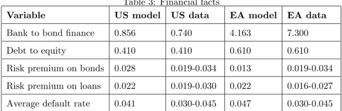
5 Comparing the US and the euro area

In this section, we review the evidence on the …nancial structure of the corporate sector in the US and the EA. We calibrate the model to capture in steady state some key di¤erences and we provide model-based answers to the questions: What are the causes of di¤erences in the

…nancial structure? What are the implications for allocations?

Some ingredients of our model, such as the degree of heterogeneity of …rms in the risk of default or the amount of uncertainty that banks are able to acquire about …rms’productivity, cannot be confronted directly with the data because of limited empirical evidence. The calibra- tion procedure described below o¤ers an indirect estimation of those unobserved characteristics of the …nancial markets based on a structural model.

5.1 Evidence on intermediation and …nancial structures

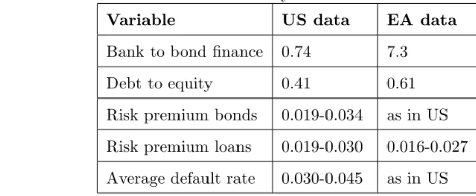
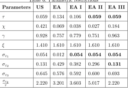
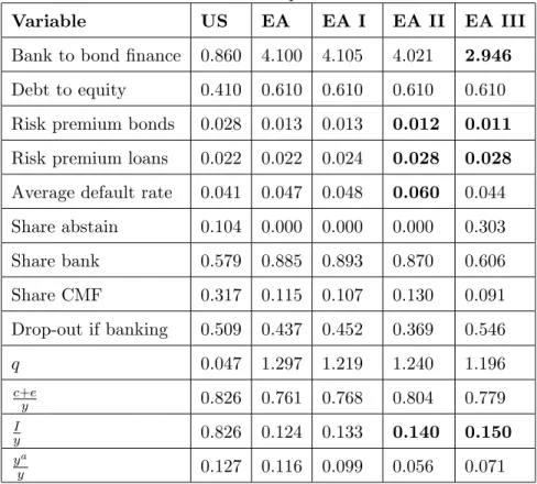
We document some corporate …nance di¤erences between the US and the EA, which we sum- marize in table 1. Some distinguishing features emerge: the ratio of bank …nance to bond

…nance and the debt to equity ratio are lower in the US than in the EA, while the converse is true for the risk premia on bank loans.

Bank …nance to bond …nance ratio. We compute the ratio of bank …nance to bond

…nance in the US and in the EA over the period 1997-2003. In the US, the ratio is 0.74. In the EA, it is 7.3, approximately ten times higher.¹⁰

1 0For the US, data are from the Flow of Funds Accounts. Bank …nance is given by bank loans plus other loans and advances, i.e. the sum of lines 22 and 23 in Table L 101. Securities are the sum of commercial paper, municipal securities and corporate bonds, lines 19, 20 and 21 in Table L 101. For the euro area, data are from the Euro Area Flow of Funds. Loans are those taken from euro area MFIs and other …nancial corporations

Debt to equity ratio. The debt to equity ratio for the US non-farm, non-…nancial corporate business sector is 0.41 over the period 1997-2003. For the EA, the same ratio for non-…nancial corporations is 0.61 over the period 1997-2002.¹¹

Risk premium on bank loans. In the US, the di¤erence between the prime rate on bank loans to business and the commercial paper rate is 298 bps over the period 1997-2003. In the EA, over the same period, the di¤erence between the interest rate on loans up to 1 year of maturity to non-…nancial corporations and the three-month interest rate, is 267 bps.¹² These numbers should be seen as upper estimates of the existing risk premia. English and Nelson (1998) report selected results from the August 1998 Survey of Terms of Business Lending in the US. The di¤erence between the average loan rate to domestic …rms (weighted by loan volumes) and the commercial paper rate emerging from the survey is 188 bps, while for the same year the di¤erence between the prime rate and the commercial paper rate is 301 bps.

The existence of higher spreads in the US relative to Europe is con…rmed by existing studies.

Carey and Nini (2004) …nd that the di¤erence between rates on bank syndicated loans and LIBOR in the US exceeds the corresponding di¤erence in the EMU by 29.8 bps. This …nding is supported by calculations of net interest margins in the banking industry by country. Cecchetti (1999) reports interest rate margins for the US in 1996 to be 268 bps. In the same year, the average interest rate margin for Austria, Belgium, Finland, France, Germany, Ireland, Italy, Netherlands, Portugal and Spain is 204.

Risk premium on corporate bonds. In the US, the di¤erence between the average yield to maturity on selected long term corporate bonds (rated Aaa and Baa) minus the 3- months Treasury Bill is 339 bps for the period 1997-2003.¹³ English and Nelson (1998) report similar spreads between bank loans rated 1 (best) and 5 (worst) in the 1998 Survey of Terms

by non-…nancial corporations. Securities are de…ned as securities other than shares issued by non-…nancial corporations.

1 1For the US, data are from the Flow of Funds Accounts. Debt is de…ned as credit market instruments (sum of commercial paper, municipal securities, corporate bonds, bank loans, other loans and advances, mortgages) over the market value of equities outstanding (including corporate farm equities), Table B.102. Masulis (1988) reports a ratio of debt to equity for US corporations in the range 0.5-0.75 for the period 1937-1984. The ratio exhibited a downward trend over the last decades due to …nancial innovations. For the euro area, data are from the Euro area Flow of Funds. Debt includes loans, debt securities issued and pension fund reserves of non-…nancial corporations. Equity includes quoted and non-quoted equity.

1 2Source: for the US, Federal Resrve Board, Table H15; for the euro area, European Central Bank, MU12 average based on country reporting to BIS.

1 3Source: Federal Reserve Board, Table H15.