Probabilistic Pose Estimation and 3D Reconstruction of Vehicles from Stereo Images

(1)

Ausschuss Geodäsie der Bayerischen Akademie der Wissenschaften

Reihe C Dissertationen Heft Nr. 857

Maximilian Alexander Coenen

Probabilistic Pose Estimation and 3D Reconstruction of Vehicles from Stereo Images

München 2020

Verlag der Bayerischen Akademie der Wissenschaften

ISSN 0065-5325 ISBN 978-3-7696-5269-7

Diese Arbeit ist gleichzeitig veröffentlicht in:

Wissenschaftliche Arbeiten der Fachrichtung Geodäsie und Geoinformatik der Universität Hannover ISSN 0174-1454, Nr. 362, Hannover 2020

(2)

(3)

Ausschuss Geodäsie der Bayerischen Akademie der Wissenschaften

Reihe C Dissertationen Heft Nr. 857

Probabilistic Pose Estimation and 3D Reconstruction of Vehicles from Stereo Images

Von der Fakultät für Bauingenieurwesen und Geodäsie der Gottfried Wilhelm Leibniz Universität Hannover

zur Erlangung des Grades Doktor-Ingenieur (Dr.-Ing.) genehmigte Dissertation

Vorgelegt von

Maximilian Alexander Coenen, M.Sc.

Geboren am 23.04.1987 in Köln

München 2020

Verlag der Bayerischen Akademie der Wissenschaften

ISSN 0065-5325 ISBN 978-3-7696-5269-7

Diese Arbeit ist gleichzeitig veröffentlicht in:

Wissenschaftliche Arbeiten der Fachrichtung Geodäsie und Geoinformatik der Universität Hannover ISSN 0174-1454, Nr. 362, Hannover 2020

(4)

Adresse der DGK:

Ausschuss Geodäsie der Bayerischen Akademie der Wissenschaften (DGK)

Alfons-Goppel-Straße 11 ● D – 80539 München

Telefon +49 – 331 – 288 1685 ● Telefax +49 – 331 – 288 1759 E-Mail post@dgk.badw.de ● http://www.dgk.badw.de

Prüfungskommission:

Vorsitzender: Prof. Dr.-Ing. habil. Christian Heipke Referent: apl. Prof. Dr. techn. Franz Rottensteiner Korreferenten: apl. Prof. Dr.-Ing. Claus Brenner

Prof. Dr.-Ing. Olaf Hellwich (TU Berlin) Tag der mündlichen Prüfung: 25.05.2020

die Veröffentlichung oder Teile daraus auf photomechanischem Wege (Photokopie, Mikrokopie) zu vervielfältigen

ISSN 0065-5325 ISBN 978-3-7696-5269-7

(5)

Abstract

The pose estimation and reconstruction of 3D objects from images is one of the major problems that are addressed in computer vision and photogrammetry. The understanding of a 3D scene and the 3D reconstruction of specific objects are prerequisites for many highly relevant applications of computer vision such as mobile robotics and autonomous driving. To deal with the inverse problem of reconstructing 3D objects from their 2D projections, a common strategy is to incorporate prior object knowledge into the reconstruction approach by establishing a 3D model and aligning it to the 2D image plane. However, current approaches are limited due to inadequate shape priors and the insufficiency of the derived image observations for a reliable association and alignment with the 3D model. The goal of this thesis is to infer valuable observations from the images and to show how 3D object reconstruction can profit from a more sophisticated shape prior and from a combined incorporation of the different observation types.

To achieve this goal, this thesis presents three major contributions for the particular task of 3D vehicle reconstruction from street-level stereo images. First, a subcategory-aware deformable vehi- cle model is introduced that makes use of a prediction of the vehicle type for a more appropriate regularisation of the vehicle shape. Second, a Convolutional Neural Network (CNN) is proposed which extracts observations from an image. In particular, the CNN is used to derive a prediction of the vehicle orientation and type, which are introduced as prior information for model fitting.

Furthermore, the CNN extracts vehicle keypoints and wireframes, which are well-suited for model association and model fitting. Third, the task of pose estimation and reconstruction is addressed by a versatile probabilistic model. Suitable parametrisations and formulations of likelihood and prior terms are introduced for a joint consideration of the derived observations and prior information in the probabilistic objective function. As the objective function is non-convex and discontinu- ous, a proper customized strategy based on stochastic sampling is proposed for inference, yielding convincing results for the estimated poses and shapes of the vehicles.

To evaluate the performance and to investigate the strengths and limitations of the proposed method, extensive experiments are conducted using two challenging real-world data sets: the pub- licly available KITTI benchmark and the ICSENS data set, which was created in the scope of this thesis. On both data sets, the benefit of the developed shape prior and of each of the individual components of the probabilistic model can be shown. The proposed method yields vehicle pose estimates with a median error of up to 27 cm for the position and up to 1.7

^◦

for the orientation on the data sets. A comparison to state-of-the-art methods for vehicle pose estimation shows that the proposed approach performs on par or better, confirming the suitability of the developed model and inference procedure.

Keywords detection, 3D reconstruction, pose estimation, CNN, active shape model, probabilis-

tic model, Monte Carlo sampling

(6)

(7)

Kurzfassung

Die Bestimmung der Pose und die 3D Rekonstruktion der Form von Objekten aus Bildinforma- tion ist eine der zentralen Aufgaben im Bereich Computer Vision und Photogrammetrie. Eine Rekonstruktion der Umgebung und bestimmter Objekte ist Voraussetzung f¨ ur aktuell relevante Anwendungen, bspw. im Bereich der Robotik oder des autonomen Fahrens. Eine ¨ ubliche Strate- gie, um mit dem schlecht konditionierten Problem der Bestimmung von 3D Objekten aus 2D Bildern umzugehen, ist die Einf¨ uhrung von a priori Wissen ¨ uber die Objekte in die Rekonstruk- tion. Hierzu wird ein 3D Modell des Objektes angenommen und so in die Daten eingepasst, dass es mit den Bildbeobachtungen ¨ ubereinstimmt. Bestehende Repräsentationen von a priori Mod- ellen sind jedoch unzulänglich und die Beobachtungen, die aus den Bildern abgeleitet werden, reichen nicht f¨ ur eine verl¨ assliche Zuordnung und Einpassung der Modelle aus. Das Ziel dieser Arbeit ist es, geeignete Beobachtungen aus den Bildern zu generieren und zu zeigen, wie die 3D Rekonstruktion von der Nutzung einer verbessertern Objektrepräsentation und einer gemeinsamen Ber¨ ucksichtigung mehrerer Beobachtungstypen profitieren kann. Vor diesem Hintergrund werden in dieser Arbeit vorranging drei wissenschaftliche Beiträge pr¨ asentiert, die zum Ziel der Rekon- struktion von Fahrzeugen aus Stereobildern entwickelt wurden. Zum Einen wird ein neuartiges differenziertes Fahrzeugmodell vorgestellt, welches eine vorausgehende Prädiktion des Fahrzeug- typs nutzt, um eine bessere Repräsentation des beobachteten Fahrzeugs zu erhalten. Des Weiteren wird ein CNN pr¨ asentiert, welches genutzt wird, um semantische Beobachtungen, wie charak- teristische Landmarken oder Kanten der Fahrzeuge, die sich als sehr n¨ utzlich f¨ ur die Modellein- passung erweisen, aus den Bildern abzuleiten. Das CNN wird außerdem dazu genutzt, um den Fahrzeugtyp sowie die Fahrzeugorientierung zu pr¨ adizieren, welche als a priori Wissen in die Mod- elleinpassung mit einfließen. Zuletzt wird ein umfassendes probabilistisches Modell f¨ ur die 3D Rekonstruktion entwickelt, welches alle extrahierten Informationen ber¨ ucksichtigt. Hierzu werden passende Parametrisierungen und Formulierungen der Likelihood-Funktionen sowie der a priori Terme vorgestellt. Ein auf stochastischem Sampling bestehendes Optimierungsverfahren wird f¨ ur die Inferenz der nicht-konvexen und unstetigen Zielfunktion entwickelt.

Umfangreiche Experimente werden anhand von zwei anspruchsvollen Datensätzen durchgef¨ uhrt um die Qualität sowie Stärken und Limitierungen des vorgestellten Verfahrens zu analysieren. Der Nutzen, der durch das vorgestellte Fahrzeugmodell sowie durch die einzelnen Komponenten des probabilistischen Modells erzielt wird, kann auf beiden Datens¨ atzen, dem KITTI sowie dem IC- SENS Datensatz, einem im Rahmen dieser Arbeit erzeugten Datensatz, nachgewiesen werden. Ein Vergleich der erzielten Ergebnisse zu verwandten Arbeiten bestätigt die Eignung des entwickelten Verfahrens f¨ ur die Posenbestimmung und die Rekonstruktion von Fahrzeugen.

Schlagworte Detektion, 3D Rekonstruktion, Posen Bestimmung, CNN, Active Shape Model,

Probabilistisches Modell, Monte Carlo Sampling

(8)

(9)

Nomenclature

Acronyms

ASM Active Shape Model

CE Cross-Entropy

CNN Convolutional Neural Network DPM Deformable Part Model DoF Degree of Freedom

FCN Fully Convolutional Network FPN Feature Pyramid Network HoG Histogram of oriented Gradients IoU Intersection over Union

MAD Median Absolute Deviation MAP Maximum a Posterior MCM Monte Carlo Methods MLP Multi-Layer Perceptron MSE Mean Squared Error OA Overall Accuracy

PCA Principal Component Analysis

RCNN Region Convolutional Neural Network RMS Root Mean Square

SfM Structure from Motion

SVM Support Vector Machine

(10)

SGD Stochastic Gradient Descent

TSDF Truncated Signed Distance Function

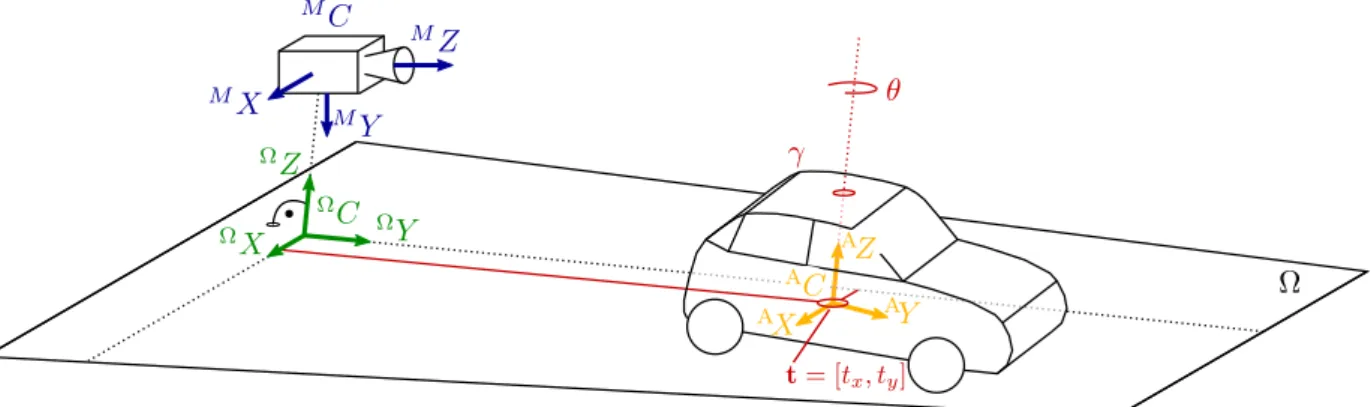
Coordinate Systems

M

C The camera model coordinate system

Ω

C The ground plane coordinate system

A

C The vehicle body coordinate system

Q Rotation matrix describing the rotation between the coordinate systems

^M

C and

^Ω

C T Vector describing the translation between the coordinate systems

^M

C and

^Ω

C

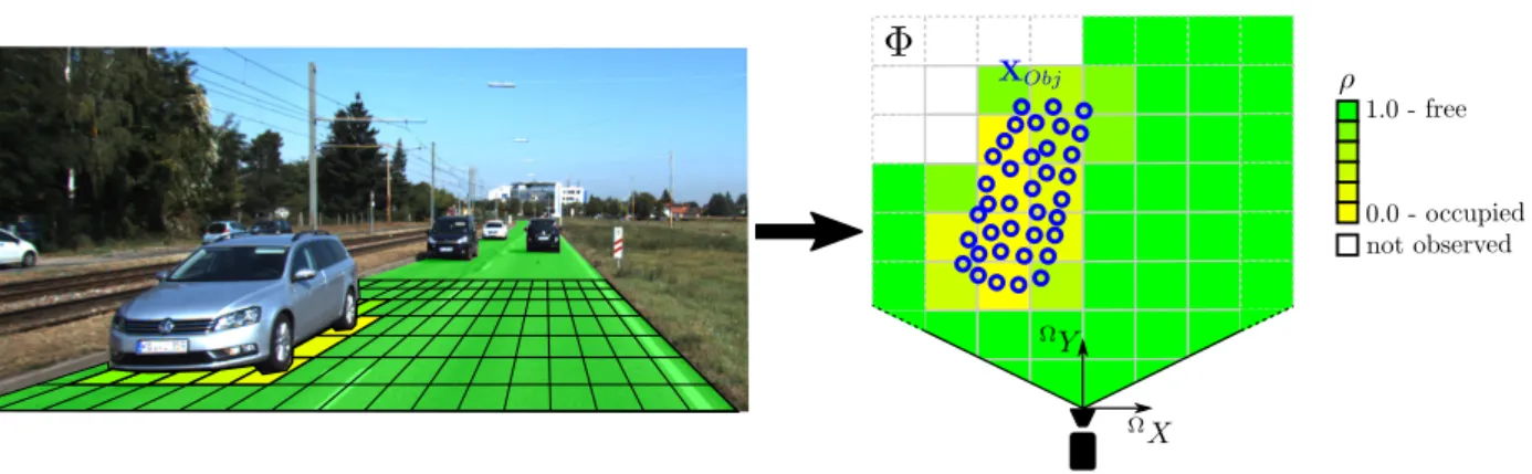
Detection

B Image bounding box

V Set of detected vehicles

Ω 3D ground plane

Φ Probabilistic free-space grid map

X

_v

The set of 3D points belonging to vehicle v

X

_Ω

The set of 3D points belonging to the ground plane Ω X

_Obj

The set of 3D points belonging to an arbitrary object v Individual vehicle detection v ∈ V

σ

_x

Depth uncertainty of a stereo triangulated 3D point ρ

_g

Probability of grid cell g ∈ Φ for being free space

o

^det

Observation vector derived from the vehicle detection with o

^det

= (X

_v

,

^l

B,

^r

B)

Active Shape Model

K Set of keypoints/vertices of the ASM

K

_A

Set of appearance keypoints of the ASM with K

_A

⊂ K

T Set of different vehicle types

(11)

M

_∆

Triangulated surface of the ASM M

_W

Wireframe of the ASM

M (γ ) Active shape model deformed according to the shape parameter vector γ M (s) Active shape model deformed and transformed according to the state vector s ν

_n

A training exemplar to learn the ASM

γ Shape vector containing the shape parameters defining a deformed ASM σ

_s

Square root of the s’th eigenvalue of the ASM

e

_s

The s’th eigenvector of the ASM m Mean shape of the ASM

CNN

Π

T

Probability distribution for the vehicle type

Π ϑ Probability distribution for the vehicle viewpoint ϑ H

_K

Keypoint probability maps

H

_W

Wireframe probability maps L

_(·)

Loss function

ϑ Vehicle viewpoint

o

^cnn

Observation vector derived from the CNN with o

^cnn

= (

^l

H

_K

,

^l

H

_W

,

^r

H

_K

,

^r

H

_W

)

Probabilistic model

s State vector s = (t, θ, γ)

t Vehicle position on the groundplane Ω

θ Vehicle heading, i.e. the rotation angle about the normal vector of the ground plane Ω o Observation vector o = (o

^det

, o

^cnn

) associated to every vehicle detection v

p(X

v

|s) The 3D likelihood

p(H

K

|s) The keypoint likelihood

p(H

_W

|s) The wireframe likelihood

(12)

p(t) The position prior p(θ) The orientation prior p(γ) The shape prior

Inference

N

_j

Number of offspring particles of iteration j n

_p

Overall number of particles

n

_b

Number of best scoring particles s

j

Set of particles of iteration j

w

_j

Importance weights of the particles of iteration j

(13)

1 Introduction

”In many cases it is sufficient to know or assume that an object owns a kind of certain regularities in order to interpret the correct 3D shape from its perspective image.”

Hermann von Helmholtz, 1867 The image based reconstruction of three-dimensional (3D) scenes and objects is a major topic of interest in computer vision and photogrammetry. While humans are able to understand and reason about 3D geometry from a short glimpse of the scene and are even capable of predicting the extends and shape of partially occluded or hidden objects, this task is very challenging for vision algorithms. The perspective projection from 3D to the 2D image plane leaves many ambiguities about 3D objects, causing their reconstruction and the retrieval of their pose and shape to be ill- posed and difficult to solve. Nonetheless, 3D scene understanding and 3D reconstruction of specific target objects has a great relevance for several disciplines such as medicine (Angelopoulou et al., 2015), augmented reality (Yang et al., 2013), robotics (Du et al., 2019), and autonomous driving (Janai et al., 2020). The motivation of this thesis is founded by applications related to the latter discipline. The highly dynamic nature of street environments is one of the biggest challenges for autonomous driving applications. The precise reconstruction of moving objects, especially of other cars, is fundamental to ensure safe navigation and to enable applications such as interactive motion planning and collaborative positioning. To this end, cameras provide a cost-effective solution to deliver perceptive data of a vehicle’s surroundings.

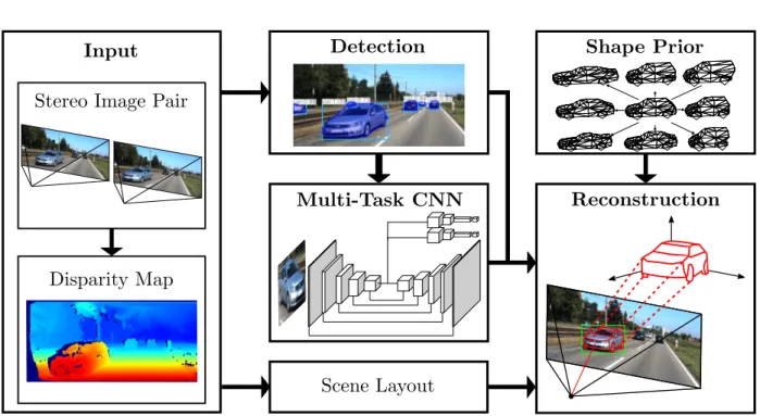
Given this background, this thesis presents a method for precise vehicle reconstruction from street- level stereo images. The poses of other vehicles w.r.t. the observing vehicle, i.e. their relative positions and orientations in 3D, can directly be derived from the reconstructions. Throughout this thesis the following definition of pose and pose related notions are used:

The notion of a 6DoF (6 degrees of freedom) object pose contains the position of the object’s ref-

erence point in form of its 3D coordinates in the reference coordinate frame as well as the 3D

orientation of the object in the same coordinate frame. In this context, the 3D orientation com-

prises three rotation angles which describe the rotation of the object body frame, which is rigidly

attached to the vehicle and centred at its reference point, w.r.t. the reference coordinate frame. In

addition to the orientation, the notion of an object’s viewpoint is introduced. In 3D, the viewpoint

describes the two rotation angles representing the elevation and azimuth of the object body frame

(18)

w.r.t. to a 3D ray, e.g. an image ray, intersecting the object reference point. The notion of a 3DoF (3 degrees of freedom) object pose in a 2D reference frame consists of two coordinates representing the position and one angle, representing the orientation. In accordance to that, a viewpoint in 2D is also represented by one angle representing the azimuth.

Geometrically, the image-based reconstruction of 3D objects from their 2D projections is an inverse problem, suffering from the ambiguous mapping inherited by the perspective projection, causing the task to be ill-posed. To address the class of ill-posed problems, a common approach is to introduce suitable constraints, e.g. derived from prior knowledge about the 3D shape, a procedure which is also called regularisation (Poggio et al., 1985). Thus, an essential strategy in work on image based object reconstruction is to establish a 3D model and align it to the 2D image plane.

To relax the requirement for precisely known object models, parametrised deformable shape priors can be formulated, increasing the set of free parameters by the parameters defining the shape. For object reconstruction usually entities such as keypoints, edges, or contours of the deformable 3D model are aligned to their corresponding counterparts localised in the image. Often, the alignment is performed by minimising the reprojection error between projections of the 3D model entities and the associated 2D image detections (Pavlakos et al., 2017; Leotta and Mundy, 2009). However, this procedure is susceptible to outliers and erroneous detections. Establishing a sufficient number of correct and sufficiently precise correspondences between model and image entities is a difficult problem. Existing approaches use model edges and contours to align them with image edges, usually derived from gradient information (Leotta and Mundy, 2009; Ramnath et al., 2014; Ortiz- Cayon et al., 2016). However, these approaches are highly sensitive to illumination, reflections, contrast, object colour and model initialisation, because these factors can cause erroneous edge- to-edge correspondences, thus prohibiting a correct model alignment. Other approaches utilise keypoint detections to be used for model alignment (Pavlakos et al., 2017; Murthy et al., 2017b;

Chabot et al., 2017). However, compared to edges, keypoints are less stable since they deliver less geometric constraints compared to edges. In addition, feature representations in the image domain lead to the effect that already small localisation errors in 2D are likely to cause large errors in 3D space. Stereo-image based approaches use 3D points reconstructed from stereo correspondences to align the 3D shape model (Engelmann et al., 2016). However, the 3D points lack the information about their exact counterpart on the model and are usually associated to the closest point on the model surface, thus demanding for a good model initialisation. Often, these difficulties define the limitations of current state-of-the art methods for model based object reconstruction as they cause such approaches to be highly sensitive to, for instance, noisy feature detection, illumination conditions, model initialisation, and/or imprecise keypoint localisation.

Following the path of model based object reconstruction, these limitations are addressed in this

thesis on the basis of stereo images, firstly by training a Convolutional Neural Network (CNN) for

the extraction of vehicle entities, such as keypoint and wireframes, as well as for the derivation

(19)

of prior knowledge, and secondly by formulating a comprehensive probabilistic model for vehicle fitting, building upon the outputs of the CNN and stereo information. A stereoscopic setup leads to less flexibility concerning data acquisition but helps to constrain the ill-posed problem of 3D reasoning. Research objectives raised in the context of this thesis are related to:

• a contrast and illumination insensitive extraction of suitable features for the model alignment.

In this context, a CNN is exploited to predict semantic vehicle keypoints and semantic vehicle wireframe edges, the latter being proposed as new feature for model fitting in this thesis.

• deriving proper state priors for object pose and shape using a CNN to establish meaningful constraints for regularising the ill-posed problem. In this context, a deep learning based prediction of the vehicle viewpoint and the vehicle type is proposed as prior information for the vehicle’s orientation and its shape, thus serving as direct observation of the target parameters,

• a probabilistic fusion of different alignment strategies both, in 2D and 3D, exploiting syn- ergistic effects anticipated from the complementary and/or redundant nature of the fused data,

• gaining robustness against noisy, false or imprecise feature detections by formulating a prob- abilistic model while properly incorporating observation and detection uncertainties and

• establishing an optimisation procedure that is insensitive to initialisation errors and local optima.

1.1 Contributions

This thesis presents a methodology for the detection and 3D reconstruction of vehicles from stereo- scopic images to finally obtain precise estimates for the vehicle’s pose and shape. Based on initially detected vehicles, the contributions of this thesis are:

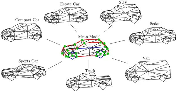
• A new subcategory-aware deformable vehicle model to be used as shape prior.

In extension to existing work, e.g. (Zia et al., 2013), where a deformable shape model is always learned for the entire class vehicle, this work presents a shape model which also learns individual modes for different vehicle subcategories. Thus, the proposed model allows a more detailed shape regularisation if an a priori prediction of the vehicle type is available. The presented shape prior leads to better constraints on the vehicle shape and evidentially also enhances the results of pose estimation.

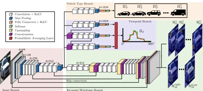
• A new multi-task CNN for the extraction of suitable features and a priori esti-

mates. The CNN simultaneously detects vehicle keypoints and vehicle wireframe edges, the

latter being proposed as new feature which is in contrast to standard gradient based edge

(20)

extraction which highly depends on illumination conditions and contrast. Furthermore, as the CNN is trained to distinguish between semantically different wireframe edges belonging to different parts/sides of the vehicle, better prospects for model-to-image-edge correspon- dences are obtained, too. To achieve this goal, a new loss function for the tasks of keypoint and wireframe prediction is introduced. The CNN also delivers a probability distribution for the vehicle’s orientation as well as the vehicle’s subcategory. For the orientation estimation, a new hierarchical classifier and a hierarchical class structure are proposed. Suitable state priors for orientation and shape are derived from the predicted probability distributions.

• A comprehensive probabilistic model for vehicle reconstruction. The probabilistic formulation combines multiple observation likelihoods, based on the keypoint and wireframe probability maps predicted by the CNN, as well as on stereo-reconstructed 3D points. Build- ing the model directly on the basis of the raw keypoint and wireframe probability maps makes the explicit association of image and model entities obsolete and reduces the impact of both, false as well as imprecise keypoint/wireframe localisations. Furthermore, state prior terms for each group of parameters, namely position, orientation and shape, are incorporated as regularisation terms based on derived scene knowledge and the probability distributions derived from the CNN. The probabilistic model is complemented with a Monte-Carlo based inference procedure similar to (Zia et al., 2013), that is tailored to reduce the sensitivity w.r.t.

parameter initialisation and local optima of the probabilistic formulation.

1.2 Thesis outline

The thesis is structured as follows. In Chapter 2, fundamental concepts for understanding the

presented methodology are given. Chapter 3 puts this work into the context of related work

on image based object reconstruction and pose estimation with a focus on vehicles as objects of

interest. A detailed explanation of the methodological contributions of this thesis is provided in

Chapter 4. The setup of the experiments to evaluate the method is described in Chapter 5, and

their results are shown and discussed in Chapter 6. A conclusion and outlook on future work are

given in Chapter 7.

(21)

2 Basics

This chapter presents mathematical and conceptual foundations that are relevant for the method- ology presented in this thesis. Sec. 2.1 provides an overview on the functionality of Convolutional Neural Networks (CNN) and presents basic architectures that are used or adapted within this the- sis. In Sec. 2.2, the Active Shape Model (ASM), used here to represent a deformable vehicle model, is described, while Sec. 2.3 introduces Monte Carlo techniques for parameter optimisation.

2.1 Convolutional Neural Networks

For several years, Convolutional Neural Networks (CNN) (LeCun et al., 1990) have shown enor- mous success in solving computer vision problems of various kinds, including image classification (Simonyan and Zisserman, 2015), object detection (Ren et al., 2015), semantic segmentation (Long et al., 2015) and instance segmentation (He et al., 2017). The basic principles and components of CNNs are outlined in this section. Furthermore, examples of selected specific CNN architectures which serve as a basis for the methodology developed in this thesis are presented.

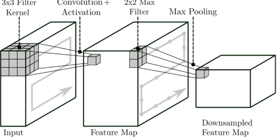
In the context of image analysis, usually the input to the neural network is a digital (single or multi- channel) image. Generally speaking, a CNN is composed of a series of convolutional layers, followed by a non-linear activation function and pooling layers. Fig. 2.1 shows an example of this structure.

In contrast to the general multi-layer perceptron (MLP) (Goodfellow et al., 2016), in which each neuron computes a linear mapping, i.e. a weighted sum, of the input and the input topology is therefore lost, CNNs preserve the spatial structure of the input image and weights are shared in the individual layers. Mathematically, this procedure leads to the utilisation of convolution filters in the convolutional layers, whose spatial size defines the receptive field of the filter and whose depth corresponds to the number channels of the respective input layer (cf. Fig. 2.1). Optionally, an additive bias is applied in every convolution, introducing one parameter to each convolution filter in addition to the filter weights. The output of the convolution filters is passed through a non- linear activation function to enable the modelling of non-linear mappings by a CNN. Examples for commonly applied activation functions are the Sigmoid function (Han and Moraga, 1995) with

sigmoid(x) = 1

1 + e

^−x

(2.1)

(22)

Figure 2.1: Schematic overview of a convolutional layer, followed by a max pooling layer. Convolu- tion filters (here: spatial kernel size of 3x3) followed by an activation function are used to create the feature maps. The kernel weights are shared for all positions of the input.

In this example, a 2x2 max pooling filter with stride 2, indicated by the dotted array, is used to create the spatially downsampled feature map.

or the Rectified Liner Unit (ReLU) function (Hahnloser et al., 2000) with ReLU(x) =







0 if x ≤ 0, x if x > 0.

(2.2) Within one convolutional layer, multiple local filter kernels are applied to all positions of the input to produce intermediate outputs which are often referred to as feature maps (cf. Fig. 2.1). The depth of the feature maps corresponds to the number of applied filter kernels. By sharing the weights of the filter kernels at all positions of the input, an enormous reduction of weight parameters that have to be learned is achieved. As shown in Fig. 2.1, the pooling layers are used to reduce the size of the feature maps and to increase the receptive field of the subsequent filters by downsampling the feature maps while preserving the spatial structure of features in the feature map. The most frequently used technique for downsampling is Max Pooling in which a max filter is applied to the input map. For downsampling the input, the step size in which the filter is shifted over the input, which is referred to as stride, has to be chosen according to the desired downsampling factor. The series of convolutional layers incl. the activation function and pooling layers is usually repeatedly applied in a CNN. Furthermore, other than as shown in Fig. 2.1, convolutional layers are often followed by additional convolutional layers before pooling is applied.

The output of a CNN can vary and depends on the task which is to be solved by the network.

For instance, in the case of image classification (Simonyan and Zisserman, 2015), at least one fully

connected layer is introduced at the end of the network which connects all its input nodes to a

number of output nodes that corresponds to the number of classes C. These neurons produce the

raw class scores s

_j

with j ∈ [1, C] as real numbers ranging from [−∞, +∞] for each class. To

(23)

normalise the raw scores such that the final scores can be interpreted as probabilities ˆ y

j

for each of the classes such that P

ˆ

y

_j

= 1, the softmax function is used (Bishop, 2006). It determines the probability ˆ y

k

for class k ∈ C by

ˆ

y

_k

= exp(s

_k

) P

j

exp(s

j

) . (2.3)

Fully convolutional networks (Long et al., 2015) and encoder-decoder networks (Ronneberger et al., 2015) differ from classification networks in that they typically do not contain fully connected layers. Such networks are used e.g. for semantic segmentation, where the task is to associate a class label to each pixel of the input image. To this end, the intermediate downsampled feature maps obtained after several convolution and pooling operations are upsampled again until they reach the target resolution by applying suitable upsampling techniques, such as e.g. bilinear upsampling or strided transposed convolutions (sometimes also called deconvolution) (Zeiler et al., 2010). The kernels of a strided transposed convolution introduce weight parameters which have to be learned during training, too (Long et al., 2015).

2.1.1 Training

Learning all network parameters w, namely all weights and biases of the filter kernels, is called training and is typically performed in a supervised manner, which means that the availability of training samples with corresponding reference data is required. The particular nature of how a training sample and its reference is defined depends on the task that is to be solved by the network.

In general, training is performed by minimising a loss function L(w) which provides a measure of how good the result of the network fits to the known reference. The definition of the loss function also depends on the task. Examples of commonly utilised loss functions are given later.

Starting from a (random) initialisation of the weights, the optimisation is performed iteratively using stochastic mini-batch gradient descent (SGD) (Goodfellow et al., 2016).

Initialisation: One way to initialise a CNN is to use random weights drawn from a Gaussian distribution. However, with fixed standard deviations, deeper models expose difficulties to converge (Simonyan and Zisserman, 2015). To overcome this problem, the Xavier (Glorot and Bengio, 2010) or the He (He et al., 2015) initialisation methods have been proposed, which choose a dynamic definition of the standard deviation in dependency on the number of input units to the convolution filters.

SGD: In the SGD procedure, a subset of the training samples, forming a mini-batch, are selected

and propagated through the network, which is called a forward pass. The loss is calculated according

to the resulting output. The gradients ∇L(w) of the loss w.r.t. to the parameters are computed in

an efficient way by exploiting the chain rule, a procedure called back-propagation (Rumelhart et

(24)

al., 1986). The new weights w

new

are derived from those of the previous iteration w

_old

according to

w

_new

= w

_old

− η∇L(w). (2.4)

The learning rate η is a hyperparameter that defines the step size in which the weights are updated.

However, plain SGD faces several problems such as local minima, noisy gradients, or regions in the loss curve in which the loss changes quickly in one direction and slowly in another. To overcome those problems, SGD with momentum is applied, which introduces running averages of gradients or variant forms of that to the weight update step. The Adam optimizer is one example of SGD with momentum which is frequently used to train CNNs and is also applied in this thesis. For a detailed exposition of this method it is referred to (Kingma and Ba, 2015).

Loss functions: The training of multi-class classification networks requires training data including a reference class for each training sample. A frequently used loss for classification tasks is the cross- entropy loss. With n training samples per mini-batch and C different classes to distinguish, the cross-entropy (CE) loss L

_CE

is calculated according to

L

_CE

= − X

N

i=1

X

C

j=1

t

_ij

log(ˆ y

_ij

). (2.5)

In Eq. 2.5, ˆ y

ij

denotes the softmax output for the i

^th

sample of the batch for the j

^th

class and t

_ij

∈ 0, 1 is a binary variable which indicates whether the sample belongs to the j

^th

class or not.

The CE loss is used in this work for the training of the classification branches of the proposed CNN.

A standard loss for training a network for regression tasks, i.e. for tasks that aim at predicting a floating value, is the mean squared error (MSE) loss L

_{M SE}

with

L

_{M SE}

= 1 N

X

N

i=1

(y

_i

− y ˆ

_i

)

²

. (2.6)

In this case, y

_i

corresponds to the reference value of the i

^th

sample while ˆ y

_i

equals the predicted output of the network. Note that for fully convolutional networks which produce pixel-wise outputs both loss functions can be applied to calculate the loss for the output of each pixel. For pixel- wise classification tasks the output has multiple channels, one for each class. In this work, the standard MSE loss is adapted by proposing a customized loss for the prediction of probability maps which contain a pixel-wise probability for the appearance of vehicle keypoints and wireframe edges, respectively.

Transfer learning: Often, it is not necessary to learn all network weights from scratch for every

new task. It is common practice to use a pre-trained network, i.e. a network that was trained for

a specific task on a specific data set, for fine-tuning or as a feature extractor for a different task

(25)

and/or data set. These strategies are summarised under the term transfer learning in the literature (Yosinski et al., 2014). When used as feature extractor, the weights of the network are usually fixed and a new classifier is learned on top of the features according to a new task. Fine-tuning refers to a strategy in which all or only some layers (typically the last few layers) of the pre-trained network are retrained together with the classification head for the new task or dataset (Donahue et al., 2014). This procedure is justified by the hierarchical structure of a CNN: while the feature maps produced by the earlier layers are more generic, independent from the data or the task, the feature maps learned at later stages represent more specific features that are more sensitive to the task and data they are trained for (Yosinski et al., 2014). This is why fine-tuning is often employed in some of the top layers only while freezing the previous layers. However, it is also possible to fine-tune all network weights using the pre-trained weights only as potentially better initialisation compared to a random initialisation. Usually smaller learning rates are applied for fine-tuning tasks as it is expected that the pre-trained weights are already relatively good. Adapting pre-trained networks for new tasks or data sets is especially helpful when only a comparably small amount of training data is available.

2.1.2 CNN Architectures

In this section, several CNN architectures which are used or adapted within this thesis are pre- sented.

VGG19

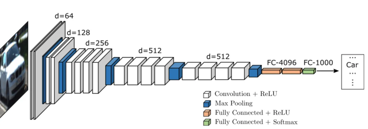
VGG19 (Simonyan and Zisserman, 2015) is a CNN architecture proposed for the task of image classification. Originally, the network was trained to classify images containing a single object into one of 1000 object classes (Russakovsky et al., 2015). An overview of the architecture is shown in Fig. 2.2. The network consists of 19 layers with weights (16 convolutional and three fully connected layers) and five pooling layers in total. The convolutional layers use d filter kernels with a spatial size of 3x3 and the ReLU as non-linear activation function. The exact numbers d of filters applied in the different layers are given in Fig. 2.2. Max pooling with kernel size of 2x2 and stride 2 is used. Three fully connected layers are applied at the end of the network: the first two layers have 4096 nodes each, while the third layer (the class layer) contains 1000 nodes, one per class. The activation function of this classification layer is the softmax function. For training, three channel colour images of size 224x224 with known object class were used (Russakovsky et al., 2015) and the cross-entropy loss function was applied. More details can be found in (Simonyan and Zisserman, 2015).

The great performance achieved by the VGG19 on the ImageNet challenge (Russakovsky et al.,

2015) is the reason why the pre-trained network released by the authors is often used as feature

(26)

d=64 d=128

d=256

d=512

FC-4096 FC-1000 ...

Car ...

...

Figure 2.2: Architecture of the original VGG19 classification network (Simonyan and Zisserman, 2015). The input is an RGB image. After several convolutional and max-pooling layers, three fully connected layers are used to produce a probability for each of 1000 classes.

extractor or as pre-trained network for fine-tuning in various subsequent tasks. The architecture of VGG19 together with its pre-trained weights serves as a basis for the multi-task CNN which is developed in this thesis and which is described in Chapter 4.

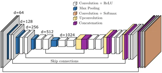
U-Net

Building upon (Long et al., 2015), the U-Net is a fully convolutional network, originally used for se- mantic segmentation (Ronneberger et al., 2015). U-Nets or U-Net-like architectures are widely used for tasks in which the output is of the same spatial extent as the input. To this end, the architecture of U-Net, which can be seen in Fig. 2.3, follows a symmetric encoder-decoder structure.

The encoder part follows the typical architecture of a convolutional network and consists of repeated

convolutional layers using a number of d filters of size 3x3, each followed by a ReLU activation

function. Also, four max pooling layers with filter size 2x2 and stride 2 are applied to decrease the

spatial resolution of the input and the subsequent feature maps by a factor of 0.5. The decoder

part is symmetric to the encoder part but replaces the max pooling layers by 2x2 upsampling

operations (in this case strided transposed convolutions are used), which spatially upsample the

feature maps by a factor 2. Skip connections, also known as bypass connections (He et al., 2016), are

used between corresponding pairs of blocks of the encoder and the decoder in order to concatenate

feature maps of the encoder with feature maps of the same size of the decoder. This allows

the subsequent convolutions to take place with awareness of the original pixels or feature maps,

respectively, and leads to better segmentation results at object boundaries. U-Net does not contain

any fully connected layers. Instead, the final layer performs convolutions with a 1x1 kernel to

map the final feature map to the desired number of classes. A 1x1 convolution corresponds to

a linear function, its output is forwarded to a non-linear activation function to produce the final

predictions which correspond to the label maps. In the original paper (Ronneberger et al., 2015),

(27)

d=64 d=128

d=256

d=512

d=1024

Figure 2.3: Architecture of the symmetric U-Net segmentation network (Ronneberger et al., 2015).

It consists of an encoder part, which performs several convolutional and max-pooling operations, and a decoder part, which performs a series of convolutions and upsampling operations. Skip connections are established between corresponding parts of the encoder and the decoder.

the softmax function is used as activation function, combined with a pixel-wise cross-entropy loss to train the network to distinguish between two classes (foreground and background). Consequently, the training procedure requires a pixel-wise reference, i.e. a label image of the same size as the input.

In this thesis, the ideas and principles of the U-Net architecture are adapted for the computation of the vehicle keypoint and wireframe heatmaps (cf. Chapter 4).

Mask RCNN

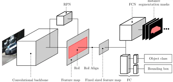
The Mask RCNN (He et al., 2017) is a CNN architecture for joint object detection and instance

segmentation. In addition to an object bounding box and the object’s semantic class the network

outputs a high-quality segmentation mask for each object. To this end, the architecture builds on

the Faster RCNN network for object detection proposed in (Ren et al., 2015), extending it with

an additional output branch to produce the instance segmentation masks. A high-level overview

of the Mask RCNN architecture is shown in Fig. 2.4. The first part of the architecture consists of

a convolutional neural network, processing the input image and producing a feature map. More

specifically, a ResNet (He et al., 2016) architecture in conjunction with a Feature Pyramid Network

(FPN) (Lin et al., 2017) is used to form the backbone. A region proposal network, which is in

essence adapted from (Ren et al., 2015), extracts regions of interests (RoI) by proposing a set of

rectangular object candidates in the feature map. A small, fixed sized feature map is created for

each RoI in the feature map using a bilinear interpolation based technique, referred to as RoIAlign

(28)

Figure 2.4: High-level overview of the Mask RCNN architecture (He et al., 2017). A three channel input image is first processed by the convolutional backbone network. A Region Pro- posal Network (RPN) is trained to extract object bounding boxes as regions of interest (RoI). The network output consists of a class label and a bounding box, produced by fully connected (FC) layers, as well as instance segmentation masks, produced by a fully convolutional network (FCN) head, for each detected object and each class.

(He et al., 2017). The head of the Mask RCNN predicts an object class and regresses an object bounding box for each RoI. In parallel, instance segmentation masks are additionally produced for each RoI and object class. In order to predict the object class of each RoI, the fixed size feature map is fed into a series of fully connected layers to predict the probability of the RoI belonging to each of a set of object classes using the softmax function. Furthermore, a FC layer is used to regress a real numbered bounding box position for the object. A FCN head is used to predict the instance segmentation masks from the same feature map using a pixel-wise sigmoid function as the activation function of the last layer.

For the training of the Mask RCNN a multi-task loss L

maskRCNN

= L

class

+L

bbox

+L

mask

is defined.

Here, the classification loss L

_class

corresponds to cross-entropy loss while the bounding box loss L

_bbox

makes use of a L1 norm of the difference of the regressed bounding boxes and the reference bounding boxes. The mask loss L

_mask

is defined as the average binary cross-entropy loss over the pixels of the bounding box. Consequently, training the Mask RCNN requires training images with annotated object bounding boxes, object class labels and an annotated instance segmentation mask for each object.

The method proposed in this thesis makes use of the Mask RCNN for the detection and precise

delineation of vehicles in the input images (cf. Chapter 4). The detected vehicles serve as input for

the developed reconstruction procedure.

(29)

2.2 Active Shape Model

The reconstruction of 3D objects from (stereo-)images, especially of objects with variable shapes, is an ill-posed problem. The use of shape priors for reconstruction constrains the problem and thus simplifies its solution. When dealing with variable object shapes, non-rigid but deformable shape priors are required, which are able to adapt to all expected possible shapes but always deliver globally plausible object instances and, thus, constrain the overall object geometry.

One technique for deformable shape modelling is the Active Shape Model (ASM) (Cootes et al., 1995), which is learned from a set of N distinct training models of an object class with a well-defined topology to capture the object’s intra-class variability. While originally applied to 2D shapes, the ASM can be used to derive a deformable shape prior in any dimension. Similar to (Zia et al., 2013), in this work a 3D ASM is learned as a deformable representation of vehicles. This mathematical explanation of the ASM focuses on learning the shape representation in 3D space.

One 3D training exemplar ν

_n

, with n = [1, N ] consists of a set of keypoints k ∈ [1, K], represented by their 3D vertex locations with ν

n

= [x

¹_n

, y

¹_n

, z

_n¹

, ..., x

^K_n

, y

_n^K

, z

_n^K

]

^T

. In this context, corresponding keypoints of different exemplars must represent the same physical point of the object. To learn the ASM, the 3D coordinates of exemplar vertices need to be represented in a commonly defined coordinate system, which has the same longitudinal axis and reference point as origin (e.g. the exemplar’s centre of mass) among all exemplars. The ASM computation is based on Principal Component Analysis (PCA) applied to the covariance matrix Σ

νν

of the keypoints of the training exemplars, resulting in the eigenvalues σ

_s²

and eigenvectors e

_s

of that matrix.

The computation of the covariance matrix requires the mean shape m which is calculated according to

m = 1 N

X

N

n=1

ν

_n

. (2.7)

The covariance matrix is computed by

Σ

_νν

= 1

N − 1 V V

^T

, (2.8)

where V is a matrix collecting the keypoint coordinates of the exemplars reduced by the mean shape:

V = [ν

₁

− m, ν

₂

− m, ..., ν

_N

− m]. (2.9)

The eigenvectors e

s

of the covariance matrix Σ

νν

encode the directions of the principal shape

deformations given the training exemplars which represent the object class. The square roots

of the corresponding eigenvalues σ

_s²

thus represent the standard deviations of the deformation in

the direction of the respective eigenvectors. A deformed object model M(γ) can be created by

(30)

a linear combination of the mean shape and the eigenvectors, the latter being weighted by their standard deviations and scaled by the shape parameters γ

_s

which are used to control the amount of deformation in each principal direction with:

M (γ ) = m + X

3K

s=1

γ

s

σ

s

e

s

. (2.10)

Defining the shape parameters γ

s

in the range of [−3, 3] allows to synthesise shape models covering 99.7% (three times the standard deviation) of the variations being present in the training set.

In practice, to reduce the dimensionality of the shape parameter space, often only the first n

s

eigenvectors corresponding to the largest eigenvalues are considered in the ASM computation, because the eigenvectors corresponding to the small eigenvalues usually represent minor shape variations and thus can be neglected (Tsin et al., 2009).

2.3 Monte Carlo based optimisation

Many tasks in the field of computer vision and machine learning involve the estimation of unknown quantities, in the following denoted as state variables s, from real-world data, i.e. from some given observations o. A probabilistic model of the task allows to estimate the unknown variables from the variables that are observed. When prior knowledge about the target phenomenon can be modelled or is available, e.g. from expert knowledge, the probabilistic model of the problem can be based on a Bayesian formulation. The Bayesian formulation utilises the prior distributions for the unknown quantities and likelihood functions relating these quantities to the observations (Doucet et al., 2001). The inference of the unknown state is based on the maximum a posterior (MAP) criterion, i.e. on maximising the posterior distribution obtained from the Bayes theorem

p(s|o) = p(o|s)p(s)

p(o) → max, (2.11)

with the likelihood term p(o|s), the prior probability p(s) and the evidence p(o). As p(o) is independent from the state variables and usually is only required as a normalisation factor to be able to interpret the posterior as a probability, the MAP estimate can be obtained without knowledge about the distribution p(o), such that p(s|o) ∝ p(o|s)p(s). For computational reasons, instead of maximising the posterior, often the negative logarithm of the posterior is minimised to derive the optimal values ˆ s for the unknown state variables. As a consequence, the state optimisation is based on minimising an objective function E, such that

ˆ s = argmin

s

E(s, o, σ

o

), (2.12)

with

E(s, o, σ

o

) = − log p(o|s) − log p(s) (2.13)

(31)

In Eqs. 2.12 and 2.13, the parameters σ

o

are used to adapt the model to the characteristics of specific data and can, for instance, be represented by observation uncertainties. In the probabilistic formulation, these uncertainties are usually considered in the likelihood terms. Standard methods for local optimisation of non-linear functions include first-order approaches based on the Jacobian of the objective or second-order approaches based on the Hessian of the objective. However, for these approaches to reach the global optimum, the objective function has to fulfil some restrictions, such as being (quasi-)convex in the continuous domain (Boyd and Vandenberghe, 2004).

The deformable 3D model fitting approach developed in this thesis is based on a non-linear, non- convex and discontinuous objective function which involves elements that are not Gaussian and thus precludes first or second-order solutions for optimisation (Doucet et al., 2001). To such prob- lems, Monte Carlo Methods (MCM) can be applied to approximate the optimal state parameters ˆ

s. A detailed description of such methods can be found in (Bishop, 2006). MCM belong to simulation-based methods and have the advantage of not requiring any assumptions about the lin- earity, convexity or statistical distribution on the model (Doucet et al., 2001). Furthermore, they are easy to implement even for the optimisation of complicated objective functions, and finally, they can be parallelised, which in principle favours their applicability to problems with real-time requirements (Kroese et al., 2014).

The central idea of MCM is to find the optimum of a potentially high-dimensional function by gen- erating a set of random samples s

ⁱ

, with i ∈ [1, n

_p

], which are called particles (Doucet et al., 2001).

If the number n

_p

of particles is large enough, such that the parameter space is densely represented by the samples, the optimum state can be estimated given the samples by ˆ s = argmin

sⁱ

E(s

ⁱ

).

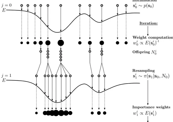
However, in a high-dimensional parameter space and/or a parameter space with potentially large parameter ranges, a dense sampling of the parameters for the particle based optimisation is compu- tationally intractable. To overcome this problem, sequential techniques can be used, in which both, particle sampling and state estimation are performed alternatively in an iterative process. Fig. 2.5 shows the scheme of a sequential MCM approach which is applied for the parameter estimation in this thesis, exemplarily depicted for a one-dimensional objective function E and for one iteration.

After initialising the first set of particles s

ⁱ₀

, each iteration j = 1, ..., n

_it

consists of of two steps, the weight computation for each of the initial particles and a resampling step, in which new particles are drawn for the next iteration based on the preceding particles and their corresponding weights.

The initial particles s

ⁱ₀

are drawn from the prior distribution p(s

₀

). When no prior information is available but the range of parameter values is known, usually an uniform distribution is applied for p(s

₀

) to draw the particles from. In each iteration j, a normalised weight w

_jⁱ

with P

i

w

_jⁱ

= 1

is associated to each particle s

ⁱ_j

. One way of estimating the weights is to define them according to

the particle’s score obtained from the objective function, such that w

ⁱ_j

∝ E(s

ⁱ_j

)

⁻¹

. The key idea of

the sequential MCM is to eliminate particles receiving low weights and consequently, to multiply

particles having high weights in the resampling step. To this end, a number of offspring N

_jⁱ

is

(32)

Figure 2.5: Schematic procedure of the MCM based optimisation for one dimension (Doucet et al., 2001). In a first step, the particles s

ⁱ₀

are initialised. In each iteration j, a weight w

_jⁱ

is calculated and associated to each particle (a larger size of the filled black circles corresponds to a higher weight). Corresponding to the weights, a number of offspring is calculated for each particle. In a resampling step, new particles are drawn based on the preceding particles and according to the number of offspring. For a detailed explanation the reader is referred to the main text.

associated to each particle (Doucet et al., 2001). In a general setting, the offspring can be deter- mined by N

_jⁱ

= w

ⁱ_j

· n

p

with P

i

N

_jⁱ

= n

p

, such that the number of offspring is larger for particles with higher weights and vice versa. Note that the numbers of offspring need to be integer values such that proper rounding operations are required for the offspring calculation just mentioned.

The resampling procedure applied in this thesis differs from this approach in that a user-defined number for the n

_b

best scoring particles is chosen. These particles are defined as seed particles for the subsequent iteration by setting the weights for these particles to

ⁿ_n^p

b

and the weights of all other

particles to 0. As a consequence, the same amount of offspring results for the best n

_b

particles,

while the remaining particles are eliminated. To generate the offspring particles for the subse-

quent iteration based on the preceding particles and the associated number of offspring, generally

speaking, an arbitrary transition function π(s

_j

|s

_j−1

, N

_j−1

) is used. In this thesis, this function

corresponds to drawing the offspring particles from a uniform distribution centred at the preceding

(33)

seed particles. By decreasing the range of the applied uniform distribution in each iteration, the

particles iteratively move towards the global minimum of the objective function E, as insinuated

in Fig. 2.5. A variant of the described procedure has already been used for 3D object modelling

in (Zia et al., 2013), where it is referred to as stochastic hill-climbing method. The iterative MCM

procedure as described above enables an efficient exploration of the search space while preserving its

applicability to arbitrary (e.g. multi-modal, non-convex, discontinuous) objective functions.

(34)

(35)

3 State of the art

To put the contributions of this thesis into context, this chapter provides an overview of related work on object reconstruction and object pose and shape recovery. The focus will be on methods that deal with objects, data and applications related to autonomous driving with vehicles as objects of main interest. In this chapter, an distinction is made between data driven approaches (Sec. 3.1) and model driven approaches (Sec. 3.2). Sec. 3.3 discusses the current state-of-the-art and summarises open questions.

On an abstract level, data driven approaches for object pose and shape recovery make use of the input data, mostly a single image, to derive an intermediate representation of the data, usually in the form of some kind of feature representation, on the basis of which the target parameters for pose and shape are inferred directly. Often, these data driven methods are coupled with approaches for object detection, such that the pose and shape estimation is a by-product of the detection or is built as an extension on top of an object detector. In contrast to that, in model driven approaches the detection and state estimation of the object are usually treated as decoupled tasks. Arbitrary object detectors are typically applied in a first step to find instances of the target objects. In a second step, a flexible shape representation of the target object based on prior knowledge is fitted to the observations of the detected instances to determine the object’s pose and shape.

3.1 Data driven approaches

Methods which extract a feature representation of the input data and train a classifier or regressor based on this feature representation to infer the target parameters for object pose and/or shape are categorised as data driven approaches in this overview. Traditionally, the feature representation is based on suitable handcrafted features, while recently almost exclusively CNNs are used for both, feature extraction and parameter estimation.

This section discusses related work on data-driven vehicle pose and shape estimation. First, ap-

proaches are reviewed which aim at estimating the vehicle viewpoint, disregarding the vehicle’s

location in 3D (cf. Sec. 3.1.1). Sec. 3.1.2 gives an overview about existing methods on 3D pose

estimation which, however, do not reason about a representation of the vehicle’s shape. Finally,

(36)

in Sec. 3.1.3 data-driven methods are reviewed that infer a joint representation for 3D object pose and shape.

3.1.1 Viewpoint prediction

A coarse estimation of the vehicle viewpoint from single images is delivered already by a number of early vehicle detection approaches. To overcome the huge variety of visual appearances of vehicles due to their intra-class variability or changes in the camera viewpoint and to handle occlusions, part-based detection approaches were introduced by Leibe et al. (2006) and Felzenszwalb et al.

(2010). They divide the object into several distinctive parts and learn a detector for each part.

Usually a global part configuration, considering the topology of the individual parts, is learned for the detection of the entire object. Pepik et al. (2015) additionally learn the viewpoint dependent arrangement of the parts in the global configuration to associate each detection already with the estimation of one of eight discrete viewpoint classes. However, the discretisation of the viewpoint into a small set of classes only allows the derivation of coarse viewpoint categories rather than the definite viewpoint angle.

Other approaches explicitly train viewpoint specific classifiers to determine a vehicle’s viewpoint.

In these approaches, the viewpoint typically also consists of a discrete number of viewpoint-bins and a classifier is trained to predict the correct bin. In (Ozuysal et al., 2009), a classifier is learned for a number of 16 vehicle azimuth classes based on SIFT-like features. Similarly, Tulsiani and Malik (2015) train a CNN to predict a class for both, azimuth and elevation angle bins, respectively. In (Su et al., 2015) a CNN is trained to predict a class for azimuth, elevation, and in-plane rotation (around the optical axis) viewpoint angles. To achieve more fine-grained results for the viewpoint, the authors distinguish 360 viewpoint classes of the detected object. More fine-grained discretisations call for extensive amounts of training data. Thus, in (Su et al., 2015) synthetic data generated from model renderings are created to train the network. However, training on synthetic data usually leads to a noticeable drop of performance when the classifier is applied to real-world data.

Summarising, most of the mentioned approaches only give a coarse indication about the viewpoint in a discretised form and the vehicle’s position in 3D, and its shape is disregarded completely.

Furthermore, the problem remains that a compromise between the classifier’s complexity and the level of detail of the viewpoint estimation has to be found in all cases. Striving for more precise viewpoint representations requires more training data.

3.1.2 3D pose prediction

One step towards capturing 3D object information from images is taken by early approaches which

internally enrich a part-based detector by linking 3D object knowledge to the parts and transferring

this information to the objects after detection. To that end, the increasing amount of freely

(37)

available CAD data is often exploited. For instance, Liebelt and Schmid (2010) treat appearance and geometry as separate learning tasks. They train an appearance based detector for object parts from real images and learn 3D geometry for each part from synthetic 3D models. Linking the detected parts with their associated 3D geometry allows an approximate estimation of 3D pose.

Similarly, Pepik et al. (2012) adapt the Deformable Part Model (DPM) of (Felzenszwalb et al., 2010). They add 3D information from CAD models to the deformable parts and incorporate 3D constraints to enforce part correspondences. Thomas et al. (2007) enrich the Implicit Shape Model (ISM) of Leibe et al. (2006) by adding depth information from training images to the ISM and transfer the 3D information to the test images, which allows the estimation of coarse 3D pose information. H¨odlmoser et al. (2013) tackle pose estimation in 3D space by defining a number of pose classes where each pose class corresponds to a different combination of viewpoint and distance classes. Consequently, the overall number of pose classes corresponds to the product of the number of distinguished viewpoint and distance bins. They train a Random Forest classifier (Breiman, 2001) to distinguish between the pose classes based on Histogram of oriented Gradients (HoG) features (Dalal and Triggs, 2005). However, due to the class-wise representation of the pose parameters, a precise and continuous pose estimation is not provided by the approaches mentioned so far.

With the emergence of CNNs the prediction of 3D object pose from images has experienced a huge boost and work on 3D object detection has expanded significantly over the last few years. A naive approach for 6DoF pose estimation would be to train a CNN to regress the target parameters from detections in the 2D image. However, regressing the pose, especially the translation, from a single image without prior knowledge is an ambiguous task. This is why typically other solutions are found in the literature, which e.g. incorporate prior scene knowledge or find alternative representations for the target pose parameters. Frequently, oriented 3D bounding boxes are estimated for the objects which implicitly contain the information about the object’s pose, i.e. their position and orientation.